HAL Id: hal-00735464
https://hal.archives-ouvertes.fr/hal-00735464
Submitted on 24 Jan 2014
HAL is a multi-disciplinary open access
archive for the deposit and dissemination of
sci-entific research documents, whether they are
pub-lished or not. The documents may come from
teaching and research institutions in France or
abroad, or from public or private research centers.
L’archive ouverte pluridisciplinaire HAL, est
destinée au dépôt et à la diffusion de documents
scientifiques de niveau recherche, publiés ou non,
émanant des établissements d’enseignement et de
recherche français ou étrangers, des laboratoires
publics ou privés.
N x N coupler uniformity in a CWDM passive star
home network based on multimode fiber: A
time-effective calculation method
Francis Richard, Philippe Guignard, Anna Pizzinat, Eric Tanguy, Hong Wu Li
To cite this version:
Francis Richard, Philippe Guignard, Anna Pizzinat, Eric Tanguy, Hong Wu Li. N x N coupler
unifor-mity in a CWDM passive star home network based on multimode fiber: A time-effective calculation
method. Journal of Optical Communications and Networking, Piscataway, NJ ; Washington, DC :
IEEE : Optical Society of America, 2012, 4 (9), pp.A48-A58. �hal-00735464�
N × N Coupler Uniformity in a CWDM
Passive Star Home Network Based on
Multimode Fiber: A Time-Effective
Calculation Method
F. Richard, Ph. Guignard, A. Pizzinat, E. Tanguy, and H. W. Li
Abstract—Optical fiber is the most appropriate medium able to meet future requirements in terms of capacity and hetero-geneity in the home network. The advantages of a passive star architecture associated with wavelength multiplexing have already been reported. For lower-cost issues, multimode fiber would be preferred, but some problems were raised related to poor uniformity of theN ×N multimode coupler when using the usual coarse wavelength division multiplexing sources. An original time-effective method is proposed, based on both simulation and calculation. Many results are provided, giving a better understanding of the behavior of theN ×N coupler when different types of sources are used, also taking into account improvement techniques such as offset launching or mode scrambling.
Index Terms—Couplers; Numerical simulation; Optical beams; Optical fiber networks; Wavelength division multiplex-ing.
I. INTRODUCTION
S
ignificant progress has been made during the past fewyears in access networks. With the continuously increas-ing bit rate on copper networks thanks to xDSL technologies, or as well with fiber-to-the-home (FTTH) deployments, it is now possible to deliver rich content up to the user’s door. The last meters to reach the user’s devices could then become the real bottleneck as the home network remains today the underdeveloped part of the network. This can be traced back to two main reasons: First, the final user could be until now satisfied with separate network segments, each carrying one type of service (digital data on Ethernet cable for Internet browsing, radio-frequency signals on coaxial cable for broadcasted television (TV)). Second, due to the variety of the delivered services and the heterogeneity of the related signals, the home network becomes the convergence point of many competing worlds, such as computers, telecommunications, and
consumer electronics, and the lack of global standardization slows down the deployment of structured solutions.
Two major challenges will drive the search for an efficient home network solution. Increasing the bit rate to meet the requirements related to the richness of the content and high interactivity is of course one of these challenges, but, as mentioned before, taking into account the heterogeneity of the signals to be delivered is also a major issue: digital signals first, such as triple-play services including data, voice, and TV, which can be encapsulated in the Internet protocol (IP), or other specific signals like HDMI (high-definition multimedia interface) links, which have to be provided separately. Analog signals, carrying digital data, also have to be taken into account: DVB (digital video broadcasting) signals for broadcasted TV delivered on different media (terrestrial, satellite, or cable TV) or radio signals exchanged between the different remote antennas that will be required for wireless connectivity when radio frequencies increase toward 60 GHz. The future structured home network must then be able to carry all these signals on a unique convergent infrastructure, and optical fiber appears as the only medium with the required performance to realize such a multiformat and future-proof network.
Two main architectures have been proposed for this structured home network. The first is based on an active star centered on a switch able to process different types of signals. This switch is connected to home network terminations, which are specific devices implemented in the different rooms to separate and deliver the various signals to the terminals with the appropriate interface. This interconnection is achieved by point-to-point multiformat links, conveying the different signals simultaneously thanks to the use of electrical and optical multiplexing. This solution has been demonstrated [1,2] and is close to industrial development. However, it could be only the first step as capacity and multiplexing possibilities remain limited on point-to-point links.
The second architecture is a longer-term solution, based on an optical passive star. This time, the network is centered on a passive N × N star coupler, which provides a broadcast architecture, and wavelength division multiplexing (WDM) is widely used to carry the different applications on specific wavelengths. The home network terminations in the different rooms contain add-and-drop filters allowing the injection or the selection of one wavelength to connect to the
n
Fig. 1. (Color online) Different topologies simultaneously imple-mented on a home network infrastructure.
desired application. This broadcast-and-select CWDM (coarse WDM) architecture provides not only enormous capacity and efficient separation between incompatible signals, but also great flexibility, as many different logical topologies may be
emulated simultaneously on such an infrastructure (Fig. 1).
This architecture has been previously demonstrated with single-mode fiber (SMF) [3] for which the CWDM technology is mature, all the required sources and filters being commercially available. However, the cost of the components used in SMF systems and some major issues related to the lack of an easy connectorization process are the main drawbacks of this solution.
The next step is then to raise the question of the possibility of implementing the broadcast-and-select CWDM architecture on multimode fiber (MMF). Actually, MMF is widely deployed in buildings and in local area networks (LANs), especially because connectorization tolerances are larger and system
costs at 0.8µm are lower. Unfortunately, the only available
CWDM sources on the market are dedicated to SMF and based on distributed-feedback (DFB) lasers with wavelengths chosen in the standardized CWDM grid, going from 1270 to 1640 nm. Experimentations on a broadcast and select CWDM network have been achieved using such sources, highlighting the problem of the power uniformity at the output ports of a multimode passive star coupler with these conditions. Two main phenomena may give rise to this degradation. First, the number of excited modes at the input ports of the coupler may be low, which affects an equal splitting of the light power between the output ports of the component. Second, the modal noise due to interference between coherent modes could lead to large variations of the output power in the time domain. The present study is focused on the first degradation cause, with the aim of better understanding of the behavior of the N × N multimode coupler used with different types of sources. Based on reported experiments, the N × N coupler and the different sources are modeled, then an original hybrid simulation and calculation method is proposed to predict the performances of the coupler in terms of uniformity when different optical sources are used. In the 1970s, early studies concerning the behavior of an N × N multimode coupler were achieved
using simplified hypotheses [4], as the computational power
was considerably lower than today. Thanks to the significant progress in this domain, we found an interest in exploring
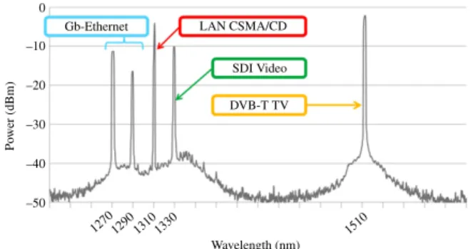
Po wer (dBm) –50 –40 –30 –20 –10 0
Gb-Ethernet LAN CSMA/CD
SDI Video DVB-T TV
1270 1290 1310 1330 1510
Wavelength (nm)
Fig. 2. (Color online) Wavelength comb of the implemented home network.
again the modeling of the coupler, expecting more advanced and accurate results.
II. PRELIMINARYEXPERIMENTS
Previous publications [5,6] have reported experiments about the broadcast-and-select CWDM architecture over MMF. The main results are reiterated in this section to illustrate the importance of the studied phenomenon.
A. The Implemented Home Network
The passive optical infrastructure was realized with
50/125µm graded-index MMF and centered on an 8 × 8 coupler
based on the same technology. Several applications have been run simultaneously on this infrastructure:
• One LAN application at 100 Mbps, using only one wavelength to emulate an optical bus, implementing a CSMA/CD (carrier sense multiple access/collision detection) medium access control. This application may be used to carry triple-play services on a shared medium.
• One point-to-point gigabit Ethernet bidirectional link, using two wavelengths.
• One unidirectional digital SDI (serial digital interface) link, using one wavelength and carrying a video program between a Blu-ray player and a TV receiver.
• One TV antenna service, broadcasting on one wavelength the entire radio-frequency (RF) TV signal from a roof antenna to several TV receivers.
All these applications have been implemented with dedi-cated wavelengths as depicted in Fig.2. Optical add-and-drop multiplexers (OADMs), usually dedicated to CWDM single-mode systems, were designed for the MMF and used as filters. A passive optical network (PON) application, an alternative for supporting the triple-play services with a perfect quality of service, was also tested. Working at 2.5/1.25 Gbps and using two wavelengths at 850 and 1300 nm, one for each direction, it could not be run simultaneously with the other applications, as only add-and-drop filters corresponding to wavelengths from the CWDM grid were available in the laboratory.
Insertion loss (dB) 20 15 10 5 0 20 15 10 5 0 1 2 3 4 5 6 7 8 Outputs 1 2 3 4Outputs 5 6 7 8
(a)
(b)
Inputs 1 2 3 4 5 6 7 8Fig. 3. (Color online) 8×8 coupler behavior with a (a) multimode and (b) single-mode source.
B. Discussion on Experimental Results
Optical sources designed for MMF links are usually vertical-cavity surface-emitting lasers (VCSELs) and Fabry–Perot (FP) lasers, emitting at the 850 and 1300 nm wavelengths. As depicted in Fig.3(a), the insertion loss of all the input/output port combinations of the 8 × 8 coupler shows an almost flat response when using a multimode source. The output power uniformity (1.8 and 2.4 dB, respectively, at 850 and 1300 nm) of the coupler is then in accordance with expected values.
Due to the lack of CWDM sources for multimode applica-tions, DFB lasers have been used, the system working then under very restricted mode launch (RML) conditions. Large variations of the coupler insertion loss appeared (Fig.3(b)), which strongly impacted the output power uniformity of the coupler with values higher than 17 dB. The optical budget for the various applications was then drastically reduced. Thanks to the large optical budget available for most applications, this degradation did not disturb the delivery of the service. Only the RF TV broadcasting was strongly affected for some combinations of input/output ports of the 8 × 8 coupler. It is clear that today, the deployment of the proposed architecture on MMF raises important questions. But the advantages of this fiber in the home network invite further investigation on the multimode N × N coupler behavior, which is described in the next sections.
III. MODEL OF THEPASSIVEN × N STARCOUPLER
One of the steps of the present study is to create a model of the N × N multimode coupler. As N × N couplers are generally made by cascading basic 2 × 2 couplers, we first focus on the 2 × 2 multimode coupler based on the main manufacturing processes. Then, this 2 × 2 model is used as the fundamental brick to obtain an N × N multimode coupler. The associated calculation methods for these models are also presented.
A. The Manufacturing Process
Passive optical couplers for MMF were mainly studied in the 1970s. Many manufacturing processes were used, leading to different passive coupler structures [7]. All these processes, based on fibers, mixing rods, or planar technologies, have been widely reported in the scientific literature. Among the early proposed solutions, it comes out that today commercially available MMF couplers are mainly based on fibers and more
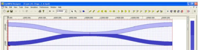
Fig. 4. (Color online) Model of the basic 2×2 coupler created with OptiBPM.
precisely on two technologies: the fused biconical taper coupler and the lapped core coupler.
The implemented 8 × 8 coupler is built from a combination of twelve 2 × 2 fused couplers. The propagation mechanisms inside this component are known [8,9]. However, the values of the opto-geometrical parameters of the component are not available as they remain confidential industrial data. In these conditions, a reliable model for a fused coupler cannot be designed.
The 2 × 2 basic coupler can also be made according to the second manufacturing process: the lapped core coupler.
Two MMFs are polished and put together [10] as shown in
Fig. 4. The structure of the remaining part of the polished
fiber core (diameter and index profile) is not modified. The weakly guiding fiber theory remains valid. Knowing their main geometrical parameters (coupling length and fiber curvature), a 2 × 2 coupler model can now be more easily created using simulation software (we used OptiBPM from Optiwave). This is one of the reasons why we focused on this coupler technology for the following steps of our work.
In order to validate simulation results by experimental measurements, we purchased 2 × 2, 4 × 4, and 8 × 8 lapped MMF core couplers, manufactured by SEDI Fibers Optiques [11], according to the second process.
B. Modeling the 2 × 2 Basic Coupler
It is difficult to obtain access to the opto-geometrical parameters of the coupler as manufacturers keep these data confidential. According to a patent held by SEDI Fibers
Optiques [12], we estimated the main parameter values. The
core and the cladding diameter of the two graded-index fibers are 50 and 125µm, respectively. The refractive indices of the core center and of the cladding are, respectively, 1.4374 and 1.452. For a 50:50 splitting ratio, the polishing depth into the core is 25µm, half of the core diameter. The bend radius of each fiber is chosen at about 20 cm and the length of the coupling area at about 1 cm, according to the SEDI Fibers Optiques patent. The created model is depicted in Fig.4.
The mesh parameters for the simulation are optimized for
an 850 nm wavelength and set at 0.25µm transversely and
0.5µm on the longitudinal axis.
Good power uniformity is obtained at the output ports of the coupler when a highly multimode optical field is injected at one input port. The optimized length of the coupling area is then investigated using a uniform input field as large as the fiber core [13]. For the modeling, the coupler guides
are laid on a 675 µm × 21,400 µm substrate. The values
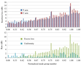
Insertion loss (dB) 0 2 4 6 8 10 12 14 16 T arm C arm 0.08 0.33 0.42 0.58 0.67 0.75 0.75 0.83 0.92 1.00 1.00 0.08 0.33 0.42 0.58 0.67 0.75 0.75 0.83 0.92 1.00 1.00 Rate (dB) 0 2 4 6 8 10 12 Excess loss Uniformity
Normalized mode group number
Fig. 5. (Color online) Modal behavior of the 2×2 model: insertion loss, excess loss, and uniformity, at 1300 nm.
accurate results. Unfortunately, these values lead to very long simulation durations, reaching about 22 h using a desktop computer with a 1 GHz dual-core processor and a 2 GB random access memory (RAM). This duration is quite prohibitive, as numerous simulations have to be achieved to observe the behavior of the coupler with different launching conditions.
C. Modal Transfer Matrices of the 2 × 2 Coupler
To overcome the problem of the simulation duration, we propose a faster calculation method, based on both simulation and calculation. This method consists of creating a modal transfer function of the 2 × 2 coupler. With this aim, the different modal fields corresponding to the fiber modes are successively launched into the coupler and their propagation through the coupler is calculated with OptiBPM software. The fiber model includes 93 and 42 linearly polarized (LP) modes respectively at 850 and 1300 nm, which form 19 and 12 mode groups, respectively. The main parameters describing the behavior of the 2 × 2 coupler, which are the insertion loss for each arm, the excess loss, and the uniformity, are reported in Fig.5. We indicate with “T” the coupler arm for which the output fiber is also the input fiber, in which the input field has been launched, while “C” corresponds to the coupler arm in which the field is coupled. The two output resulting fields, from each input field, are submitted to the process described below.
Anywhere inside the fiber, any field U¡r,ϕ, z¢, where ¡r,ϕ, z¢ are the cylindrical coordinates, may be written as a linear
combination of the fields un¡r,ϕ¢ related to the n LP modes
constituting an orthogonal set: U¡r,ϕ, z¢ =X
n
cn(z) × un¡r,ϕ¢. (1)
The cn complex coefficient is the weight associated with
the mode number n. This weight can be obtained by a modal
Fig. 6. (Color online) Modulus (left) and phase (right) matrices of the T arm of the 2×2 coupler, at 850 nm.
decomposition, calculated with the following overlap integral:
cn(z) = Z2π 0 Z∞ 0 U ¡r,ϕ, z¢ × u∗ n¡r,ϕ¢ × rdrdϕ. (2)
The set of the n weights forms a column vector, representing any field. The propagation of this field, through the 2 × 2 coupler, results in two new vectors corresponding to the two output fields on the two output arms. In particular, this process may be achieved with the fields corresponding to each LP mode and successively launched in the coupler. The resulting output vectors on one arm constitute the columns of an n × n matrix, which will be named the modal transfer matrix of the considered arm of the 2 × 2 coupler.
Separating the modulus from the phase of their complex values allows a graphical representation of the matrix. The transfer matrix of a 2 × 2 coupler is shown as an example
in Fig. 6. For the modulus matrix, a color scale gives a
representation of the modulus from the lower (blue) to the higher (red) values. The broadening of the diagonal, with a large yellow area, shows the mode coupling phenomenon inside the component. For the phase matrix, two colors are chosen: red for the positive values, blue for the negative ones. Its graphical representation shows symmetry with respect to the main diagonal.
D. Matrix Calculation for the N × N Coupler
For any input field, the two output fields are given by the fast and easy matrix calculations:
(OT) = [T] × (I), (3)
(OC) = [C] × (I), (4)
where¡OT¢ and ¡OC¢ are respectively the modal decomposition vectors of the output fields from the T and the C arms, (I) is the modal decomposition vector corresponding to the input field, and [T] and [C] are respectively the n × n modal transfer matrices of complex weight values of the T and the C arms, for a given wavelength.
A calculation method had already been used at the end of the 1970s [7]. 3 × 3 matrices were then created from intensity measurements. The present approach provides more accuracy with a calculation achieved on 93 × 93 (at 850 nm) and 42 × 42
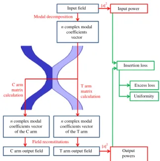
Input field x Input power 2 x2 Modal decomposition n complex modal coefficients vector n complex modal coefficients vector of the C arm n complex modal coefficients vector of the T arm C arm matrix calculation T arm matrix calculation Field reconstitutions
C arm output field T arm output field Output powers
Excess loss Uniformity Insertion loss
Fig. 7. (Color online) Algorithm for the calculations on the 2 ×2 coupler.
Input field
Stage 1 Stage 2 Stage 3
4 × 4 coupler 8 × 8 coupler 8 paths: TTT TTC TCT TCC CTT CTC CCT CCC
Fig. 8. (Color online) An N×N coupler schematic.
(at 1300 nm) complex value matrices, taking into account the field phase, thanks to the available high computational power. A Matlab program has been written integrating all the operations: modal decomposition, matrix calculation, field, and power calculation. The system parameters are then given for the 2 × 2 coupler model. The calculation steps are depicted in Fig.7.
We make the assumption that the N × N coupler results from a combination of identical 2 × 2 couplers, organized in three stages, as depicted in Fig.8. The matrix calculation is extrapolated to the N × N coupler by multiplying the basic coupler matrices, thanks to the system linearity [7]. The output fields from the 8 × 8 coupler are computed using the following relation:
(Ox yz) = [z] × [y] × [x] × (I), (5)
where x, y, and z represent either the T or the C arm of the first, the second, and the last stage, respectively; [x], [ y], and
–3 –2 –1 0 0 5 10 15 20 1 2 3 –3 –2 –1 0 1 2 3 –3 –2 –1 0 1 2 3 Dif ference (%) T C Radius (µm) Radius (µm) 0 5 10 15 20 Radius (µm) 0 5 10 15 20 TT TC TTT TTC CTT CCC TCT CTC TCC CCT
Fig. 9. (Color online) Comparison between simulation and matrix calculation results for the 2×2 (left) and the 8×8 (right) couplers.
[z] are their associated n × n modal transfer matrices. (I) is the modal decomposition vector corresponding to the input field, and¡Ox yz¢ is the vector corresponding to the field at the output of the x yz path. The eight separated paths from one input to the different outputs are shown in Fig.8.
The Matlab program is adapted for all the 2 × 2, 4 × 4, and 8 × 8 coupler calculations. Compared with the 22 h spent for one-stage simulation, only 4 and 2 h (respectively at 850 and 1300 nm) are now needed for the three-stage calculation, for one given input field. Seven simulations were needed to observe the behavior of the three stages with one input field. The gain is then more than 6 days per input field.
IV. BEHAVIOR OF THEMODEL
Modal transfer matrices model the N × N coupler. A fast calculation method has been proposed for its behavioral study. In this part, we now compare and analyze the simulation and the calculation results in order to validate the calculation method based on a modal transfer matrix. Then, the behavior of the 2 × 2 model will be checked for some cases of emitted beam models from real sources. Furthermore, the behavior of the N × N model will be extrapolated for the sources of interest for our application. Finally, these last results will be compared to experiments.
A. Validation of the Matrix Calculation Method
Simulations and matrix calculations with the same input fields have been run simultaneously. Input Gaussian fields with different radius values smaller than the fiber core radius were chosen. The comparison of the insertion loss obtained by the two methods reveals a slight difference. A difference lower
than 3% for all paths can be observed, as shown by Fig.9for
the 2 × 2, 4 × 4, and 8 × 8 couplers.
Considering these results, we have assumed that the matrix calculation method was validated and could be used in place of simulation.
B. The 2 × 2 Coupler Behavior
In this section, we observe the behavior of the basic coupler when beam models closer to real optical sources are used. In a first step, we choose a Gaussian input field with different widths, as it represents the emitted beam of most of the real optical sources. Then, we focus on the particular case of the VCSEL. For a better understanding, a modal decomposition is
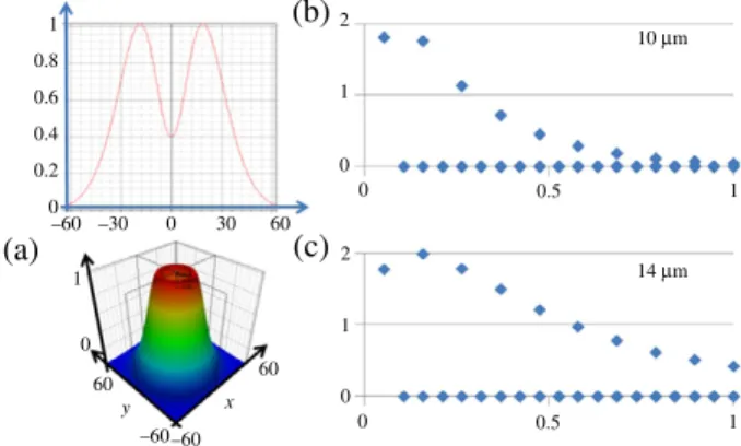
0 0.2 0.4 0.6 0.8 1 1 0 60 60 –60 –60 –30 –60 y x 0 0 0.5 1 2 0 1 2 1 0 0.5 1 24 µm 10 µm
(a)
(b)
(c)
0 30 60Fig. 10. (Color online) (a) 1D, 2D, and 3D Gaussian field representa-tion and its modal decomposirepresenta-tion for a (b) 10 µm (single-mode VCSEL beam) and (c) 24 µm (LED beam) radius. (b, c: vertical axis: weight modulus; horizontal axis: normalized mode group number).
represented by a graph showing the cartography of the excited modes. The associated mode weight modulus is given for the normalized mode group number, at 850 nm.
1) The Input Gaussian Field: The Gaussian field, with different radius, represents the emitted field of various real optical sources. According to the scientific literature, a Gaussian field as large as the fiber core diameter emulates the field emitted by a LED [13,14]. The modal decomposition of this field just after launching (Fig. 10(c)) shows a highly multimode field as a great number of modes is excited in the fiber. A 1 to 3µm width Gaussian field represents the FP and
DFB near-field emissions [15]. The bias current impacts on
the VCSEL emitted field. For a low current close to the lasing
threshold, the VCSEL emits a 6 to 12µm width circular base
Gaussian field. Figure10(b)shows the modal decomposition of
this weakly multimode field, as only a few modes are excited (about 5 modes of 93).
The main parameters of the 2 × 2 coupler, at 850 nm,
are depicted in Fig. 11. For all the simulated sources, the
excess loss remains lower than the manufacturer specifications (<1 dB). With the input field emitted by FP and DFB lasers, the uniformity is very poor, demonstrating bad performance. The results are more favorable with a VCSEL biased by a low current. As expected, the best result, lower than 1 dB, is obtained with a LED.
2) The Input Annular Field: For higher bias currents, the VCSEL emits an annular field, with a circular base diameter of about 15µm [16]. The resulting propagating field
in the fiber is as depicted in Fig. 12(c). Comparing their
modal decomposition, an annular field with a smaller radius
(Fig. 12(b)) excites quite the same modes in the fiber as a
Gaussian field with the same radius (Fig.10(b)).
As depicted in Fig.13, the model meets the manufacturer
specifications, in terms of uniformity, for input field radius
broader than 10µm. If this radius is lower than 20µm, the
excess loss is in accordance with the specifications.
For a VCSEL beam with a radius of approximately 15µm,
the performance in terms of uniformity is close to the LED’s 0 0 5 10 15 20 25 1 2 3 4 5 6 7 8 9 10 Rate (dB) Radius (µm) FP, DFB VCSEL DEL T arm insertion loss C arm insertion loss Excess loss Uniformity "SEDI-Fibers" specifications: excess loss and
uniformity <1 dB
Fig. 11. (Color online) 2×2 coupler behavior with variable Gaussian input fields radius.
1 0 60 60 –60 –60 –30 –60 y x 0 0 0.5 1 2 0 1 2 1 0 0.5 1 14 µm 10 µm
(a)
(b)
(c)
0 0.2 0.4 0.6 0.8 1 0 30 60Fig. 12. (Color online) (a) 1D, 2D, and 3D annular field representation and its modal decomposition for a (b) 10 µm and (c) 14 µm radius (multimode VCSEL beam). (b, c: vertical axis: weight modulus; horizontal axis: normalized mode group number).
Rate (dB) Radius (µm) T arm insertion loss C arm insertion loss Excess loss Uniformity "SEDI-Fibers" specifications: excess loss and
uniformity <1 dB 0 1 2 3 4 5 6 7 0 5 10 15 20 25
Fig. 13. (Color online) 2×2 coupler behavior with variable annular input field radius.
performance. This is confirmed by observing Figs. 10(c)and
12(c): The two mode cartographies exhibit a large number of excited modes of the most orders, representative of launching by a multimode source.
The 2 × 2 model and the real basic coupler have similar behavior. Thus, we assume that this model is validated and that an extrapolation may be done to the 4 × 4 and 8 × 8 couplers.
TABLE I
CALCULATEDEXCESSLOSS(dB)OF THEN × N COUPLERS,
COMPARED TO THEMANUFACTURERSPECIFICATIONS,AT
850 nm. Coupler 2×2 4×4 8×8 Manufacturer specifications <1 <3 <4 LED model 0. 84 0.68 0.77 VCSEL model 0.11 0.44 0.49 Notes. dB=decibel. TABLE II
CALCULATEDUNIFORMITY(dB)OF THEN × N COUPLERS,
COMPARED TO THEMANUFACTURERSPECIFICATIONS,AT
850 nm. Coupler 2×2 4×4 8×8 Manufacturer specifications <1 <2 <3 LED model 0.4 0.93 3.35 VCSEL model 0.7 1.15 3.57 Notes. dB=decibel.
A narrow emitting field is the cause of the poor uniformity between output ports. Indeed, this kind of field does not excite a sufficient number of modes. Thus, only broader fields are considered in the next step of the study.
C. The 4 × 4 and 8 × 8 Couplers’ Behavior
The proposed approach can now be extended to 4 × 4 and 8 × 8 couplers. Concerning the optical sources, only LED and VCSEL will be considered: the LED can be seen as a reference, leading to excellent performance for the coupler uniformity, and the VCSEL as it is the targeted type of optical source for WDM applications on a MMF infrastructure. The calculated performances, in terms of excess loss and uniformity, at
850 nm, are reported in TablesIandIIand compared to the
values obtained with the 2 × 2 coupler.
For a better understanding of the coupler behavior, the weight of the excited modes, obtained from the modal decomposition, is considered, and its evolution is observed at each output port of the basic 2 × 2 couplers constituting the different stages of the N × N coupler (Figs.14and15).
1) With the LED: The calculated excess loss, for the 2 × 2,
4 × 4, and 8 × 8 couplers, is less than 1 dB (Table I).
The uniformity is in accordance with the manufacturer
specifications for the first two components (Table II). The
uniformity of the 8 × 8 coupler is also acceptable, being only 0.35 dB higher than the specification. The modal decomposition is achieved for the different stages of the 8 × 8 coupler, for a large Gaussian field, emulating the emission of the LED. The initial cartography of the excited modes is depicted in Fig.10(c).
Considering that the 2 × 2 basic couplers building the N × N coupler are all identical, we assume that the performances of the eight paths from the first input port to the eight output ports of the N × N coupler may be generalized to all the paths between any input and output port of the coupler (Fig.8).
Stage 1 Stage 2 Stage 3
0 0.5 1 1.5 0 0.5 1 1.5 0 0.5 1 0 0.5 1 T TT TTT TTC TCT TCC CTT CTC CCT CCC TC CT CC C
Fig. 14. (Color online) Cartographies of the excited modes at the output ports of each stage with an input Gaussian field (vertical axis: weight modulus 0.5/line; horizontal axis: normalized mode group number).
Stage 1 Stage 2 Stage 3
0 0.5 1 1.5 0 0.5 1 0 0.5 1 T TT TTT TTC TCT TCC CTT CTC CCT CCC TC CT CC C 0 0.5 1 1.5
Fig. 15. (Color online) Cartographies of the excited modes at the output ports of each stage with an input annular field (vertical axis: weight modulus 0.5/line; horizontal axis: normalized mode group number).
The cartography of the excited modes at the output of the T and C arms of the first 2 × 2 coupler (stage 1) is given by the two graphs of the first column of Fig.14. The resulting fields for
the second stage are represented by their modal decomposition on the four graphs of the second column. Finally, the eight graphs of the third column correspond to the fields at the eight outputs of the coupler. Even if the phase of the associated mode coefficients is not taken into account, comparing these cartographies allows a tendency of the modes’ behavior to be observed.
Considering a strong mode mixing inside the coupler and the large number of excited modes, it is very difficult to predict the behavior of each mode separately, taking into account the different propagating paths. However, as the more impacting effect results from coupling between adjacent modes inside mode groups, assumptions can only be made on coupling between these mode groups.
Highest-order mode groups suffer the largest attenuation. Indeed, these modes are those which propagate the closest to the core–cladding interface, so they are subsequently very sensitive to the guide bends.
The light power is mainly carried by the lowest-order mode groups. These modes are close to the center of the core and thus less impacted by the guide bends. We focus on the first two groups, each including only one mode. These modes are represented by the first two points on the left side of the graphs
of Fig.14. Focusing on the fundamental and the second modes
we observe that the weight of one of the two modes offsets the weight of the other, carrying together the same quantity of power in each path of the coupler.
2) With the VCSEL: The beam emitted by a VCSEL is narrower than the LED’s beam. But this source exhibits promising features in terms of cost, modulation bandwidth, and emitted power.
When a VCSEL is used, the coupler shows lower excess loss (Table I) due to fewer leaks into the cladding. Actually, the highest-order mode groups are less excited by a VCSEL than by a LED (Fig.12(c)compared with Fig.10(c)).
This RML condition does not impact significantly the uniformity of the couplers (TableII).
The modal analysis reveals again that offsetting occurs between the weights of the two first modes (Fig.15). Although the LED and VCSEL achieve restricted and overfilled mode launching (RML and OFL), respectively, modal observation gives quite similar results for both sources.
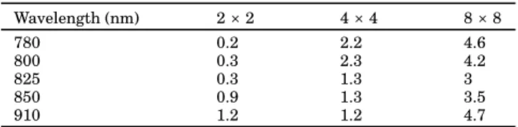
D. Experimental Validations
The calculated results given in the previous section are in accordance with the manufacturer specifications. However, as far as possible, it is relevant to compare these results with measurements carried out with real sources and real couplers. These measurements were done using VCSEL prototypes at different wavelengths: 780, 800, 825, 850, and 910 nm. The uniformity, measured with a VCSEL under RML conditions
and reported in TableIII, is as expected worsened compared
with the manufacturer measurements achieved under OFL conditions (2.1 dB at 850 nm). However, the calculated values are close to our measurements for the different N × N
TABLE III
MEASUREDUNIFORMITY(dB)OF THEN × N COUPLERS,
WITHVCSELS Wavelength (nm) 2×2 4×4 8×8 780 0.2 2.2 4.6 800 0.3 2.3 4.2 825 0.3 1.3 3 850 0.9 1.3 3.5 910 1.2 1.2 4.7 Notes. nm=nanometer, dB=decibel. 0 0.5 1 0 0.5 1 0 0 0.5 1 0 0.5 1 0 0.5 1 0 0.5 1 0.5 1 0 0.5 1 0 µm 12 µm 6 µm 18 µm
(a)
(b)
(c)
(d)
Fig. 16. (Color online) (a) Modal distribution for a narrow Gaussian launching on the center of the core fiber and with (b) 6, (c) 12, and (d) 18 µm offsets, at 850 nm. (vertical axis: weight modulus; horizontal axis: normalized mode group number).
couplers and remain in accordance with the manufacturer specifications, provided at 850 nm.
V. IMPROVING THEUNIFORMITYWHENUSING
NARROW-SPECTRUMSOURCES
A MMF system has been designed for the 850 nm wavelength domain. Implementing a home network in this window would then decrease the system’s costs with the use of VCSELs at different wavelengths. However, due to the lack
of standardization for CDWM applications at 0.8µm, sources
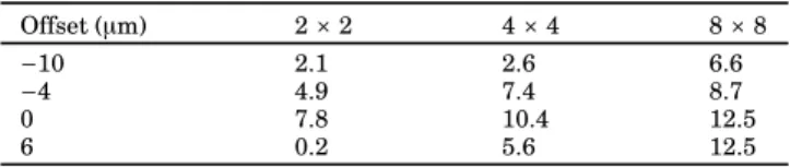
at specified wavelengths and their associated filters are not today available in that window. In the first section of this paper, we have reported the bad performance of the couplers in terms of uniformity when narrow-spectrum light sources such as FP or DFB lasers were used. Some solutions or devices have been proposed, commercially or in the literature, to excite a greater number of modes in the MMF and thus improve the performance of the N × N coupler. They are mainly based on the introduction of an offset from the core center when injecting the light or inserting a mode scrambler into the light path. It is then relevant to test the capability of the simulation and calculation tool we have proposed to highlight the gain provided by these solutions.
A Gaussian beam with a 10µm base diameter is chosen for
modeling a narrow-spectrum source, as it corresponds to the field injected in the MMF by a FP or DFB laser, as well as by the SMF pigtail of a CWDM source. This beam excites only the
fundamental mode of the MMF, as depicted in Fig.16(a). The
performances of the N × N couplers, in terms of uniformity, for the considered field, are reported in TableIV.
TABLE IV
CALCULATEDUNIFORMITY(dB)OF THEN × N COUPLERS,
WITHINPUTNARROWGAUSSIANFIELDWITHDIFFERENT
OFFSETS,AT850 nm Offset (µm) 2×2 4×4 8×8 −10 2.1 2.6 6.6 −4 4.9 7.4 8.7 0 7.8 10.4 12.5 6 0.2 5.6 12.5 Notes.
nm=nanometer, µm=micrometer, dB=decibel.
Uniformity (dB) –20 –15 –10 –5 0 0 5 10 15 20 5 10 15 20 Offset (µm) Stage 1 Stage 2 Stage 3
Fig. 17. (Color online) Output power uniformity of the 2×2, 4×4, and 8×8 couplers for an input narrow Gaussian field with different offsets at 850 nm.
A. Offset Launching
The impact of a launch with offset from the center of the fiber core on the input modal distribution has already been shown [17]. Figures16(b)–16(d)show examples of the modal distribution for different offset values. As anticipated, we may observe the increasing number of excited modes when increasing the offset.
Results are obtained using our proposed matrix calculation method. The impact of the offset on the uniformity of the couplers is shown in Fig.17. Uniformity is improved for three offset values highlighted in TableIV: −10, −4, and 6µm, with the best result at −10µm.
We may observe that offset launch does not increase the excess loss (0.8, 1.6, and 2.3 dB, respectively, for 2 × 2, 4 × 4, and 8 × 8 couplers), as mainly low-order modes are excited for offsets between −14 and 14µm.
Although the offset launch may increase the performance of the couplers in terms of uniformity, it remains a complex process difficult to implement in a marketable product. On the contrary, devices such as mode scramblers are commonly found on the market.
B. Mode Scrambling
One possibility to realize a mode scrambler consists of applying stresses to the fiber, for instance, by way of periodic bends, as depicted in Fig.18. A model describing such a device has been created. The amplitude of the bends vary from 75 to 175µm and are applied to the fiber with a 25µm periodicity,
3000 2300 75 to 175 125 13,600 18,900
Fig. 18. (Color online) Model of a mode scrambler (dimensions are in µm) . Uniformity (dB) 0 3 6 9 12 15 18 Stage 1 Stage 2 Stage 3 0 25 50 75 100 125 150 175 Bend amplitude (µm)
Fig. 19. (Color online) Output power uniformity of the 2×2, 4×4, and 8×8 couplers with an input narrow Gaussian field centered on the core fiber and passed through the mode scrambler with different bend amplitudes, at 850 nm.
a bend amplitude equal to zero corresponding to a straight fiber. Simulations are run with the OptiBPM software for the considered input field. Afterward, the resulting field is submitted to the matrix calculation method in order to study the behavior of the couplers.
The impact of the mode scrambler on the uniformity of the couplers is shown in Fig.19. For the strongest stress values (>150µm), the uniformity is improved, with a gain of 1.9, 2.5, and 1.4 dB, respectively, for the 2 × 2, 4 × 4, and 8 × 8 couplers. Due to the low order of the excited modes, the excess loss of the 4 × 4 and 8 × 8 couplers remains respectively lower than 0.2 and 1.3 dB and is almost equal to zero for the 2 × 2 coupler.
C. Combination of Offset Launching and Mode Scram-bling
The two previously described solutions are not exclusive and may be combined. The same input field model is launched into the simulated mode scrambler with various offset values. The resulting field at the output of the mode scrambler acts as input data for the matrix calculations representing the coupler behavior. Some results are reported on the graphs in Fig.20.
In the previous section the best results with only an offset
launch were obtained with an offset of −10 µm. This time,
when combining offset launch with mode scrambling, increased performances are observed for 5 and 10µm offsets (Figs.20(c)
0 0 25 50 75 100 125 150 175 0 25 50 75 100 125 150 175 0 25 50 75 100 125 150 175 0 25 50 75 100 125 150 175 4 8 12 16 20 0 4 8 12 16 20 0 4 8 12 16 20 0 4 8 12 16 20 (a) (b) (c) (d) Stage 1 Stage 2 Stage 3
Fig. 20. (Color online) Output power uniformity of the 2×2, 4×4, and 8×8 couplers with an input narrow Gaussian field launched with (a)−10, (b)−5, (c) 5, and (d) 10 µm offsets and passed through the mode scrambler, with different bend amplitudes, at 850 nm. (vertical axis: uniformity (dB); horizontal axis: bend amplitude (µm)).
are then 7 and 10 dB, respectively, for 5 and 10µm offsets. The excess loss increases for the 4 × 4 and 8 × 8 couplers (1.5 and 2.6 dB) but remains low.
VI. CONCLUSION
In this paper, we have highlighted the issues related to the implementation of WDM in an N × N passive star home network based on MMF.
We have proposed a time-efficient tool, based on simulation and calculation, to get a better understanding of the encountered phenomena, with a time saving of more than 6 days per studied input field. The calculation is based on the modal transfer matrices of a 2 × 2 MMF coupler. 93 × 93 and 42 × 42 complex values form the matrices with dimensions corresponding to the LP mode number encountered at the respective 850 and 1300 nm wavelengths. An extrapolation has also been proposed for N × N components. Many results have been reported; we have shown in particular the impact of the optical source launching parameters on the coupler uniformity, which is a major issue to guarantee the required optical budget for the different implemented services. A narrow beam can damage the 8 × 8 coupler performance by causing a more than 10 dB uniformity value. The best behavior, corresponding to a uniformity value of about 3 dB, has been obtained with the largest transverse field. This beam model corresponds to transverse multimode sources, such as VCSEL and LED, the only currently available active components.
The proposed tool has been validated by experimental measurements obtained with real sources, in particular VCSELs emitting at different wavelengths in the 850 nm window and 2 × 2, 4 × 4, and 8 × 8 couplers. Indeed, the calculated uniformity of the 8 × 8 coupler model, excited by a 850 nm VCSEL beam model, is equal to 3.57 dB, very close to the 3.5 dB measured value. We have also shown the possibility to apply this tool to the study of injection techniques as the offset launch or to different devices as mode scramblers.
The use of WDM on MMF remains limited today. It is mainly used to increase the bit rate on point-to-point links, generally for LAN or data center applications. The future needs for a
home network providing performances and flexibility while maintaining an acceptable cost will highlight the interest for a high-capacity MMF solution.
This work is a first step for a better understanding of the behavior of a multimode N × N coupler used in a CWDM scenario. It has to be carried on, keeping in perspective the design optimization of low-cost optical sources suited for a CWDM multimode passive star home network, while providing inputs for a standardization process including the extension
of the CWDM grid toward shorter wavelengths in the 0.8µm
window.
ACKNOWLEDGMENT
This work was partly supported by the European EU FP7 ICT ALPHA project and will be continued thanks to the RLDO French collaborative project, from January 2012.
REFERENCES
[1] J. Guillory, Ph. Guignard, F. Richard, L. Guillo, and A. Pizzinat, “Multiservice home network based on hybrid electrical and opti-cal multiplexing on a low cost infrastructure,” in Access Networks and In-house Communications (ANIC), Karlsruhe, Germany, June 2010, AWB5.
[2] J. Guillory, A. Pizzinat, Ph. Guignard, F. Richard, B. Charbon-nier, P. Chanclou, and C. Algani, “Simultaneous implementation of gigabit Ethernet, RF TV and radio mm-wave in a multiformat home area network,” in 37th European Conf. and Exhibition on Optical Communication (ECOC), Geneva, Switzerland, Sept. 2011, P133.
[3] Ph. Guignard, H. Ramanitra, and L. Guillo, “Home network based on CWDM broadcast and select technology,” in 33rd Euro-pean Conf. and Exhibition on Optical Communications (ECOC), Berlin, Germany, Sept. 2007, P133.
[4] K. Ogawa, “Simplified theory of the multimode fiber coupler,” Bell Syst. Tech. J., vol. 56, no. 5, pp. 729–745, 1977.
[5] F. Richard, Ph. Guignard, A. Pizzinat, L. Guillo, J. Guillory, B. Charbonnier, T. Koonen, E. Ortego Martinez, E. Tanguy, and H. W. Li, “Optical home network based on an N×N multimode fiber architecture and CWDM technology,” in Optical Fiber Com-munication Conf. (OFC), Los Angeles, CA, Mar. 2011, JWA080. [6] F. Richard, Ph. Guignard, J. Guillory, L. Guillo, A. Pizzinat,
and T. Koonen, “CWDM broadcast and select home network based on multimode fibre and a passive star architecture,” in Ac-cess Networks and In-house Communications (ANIC), Karlsruhe, Germany, June 2010, AWB3.
[7] A. K. Agarwal, “Review of optical fibre couplers,” Fiber Integr. Opt., vol. 6, no. 1, pp. 27–53, 1987.
[8] M. K. Barnoski and H. R. Friedrich, “Fabrication of an access coupler with single-strand multimode fiber waveguides,” Appl. Opt., vol. 15, no. 11, pp. 2629–2630, 1976.
[9] C. Yeh, W. P. Brown, and R. Szejn, “Multimode inhomogeneous fiber couplers,” Appl. Opt., vol. 18, pp. 489–495, 1979.
[10] Y. Tsujimoto, H. Serizawa, K. Hattori, and M. Fukai, “Fabrica-tion of low-loss 3 dB couplers with multimode optical fibres,” Electron. Lett., vol. 14, no. 5, pp. 157–158, 1978.
[11] SEDI Fibers Optiques, Multimode couplers datasheet [Online]. Available: http://www.sedi-fibres.com/coupleurs-multimodes_5_ 67.html.
A58 J. OPT. COMMUN. NETW./VOL. 4, NO. 9/SEPTEMBER 2012 Richard et al.
[12] F.-L. Malavieille, “Optical fiber coupler-distributer and method of manufacture,” US patent US4720161.
[13] A. W. Snyder and J. D. Love, Optical Waveguide Theory. Chap-man and Hall, 1983, ch. 20, pp. 420–441.
[14] R. Borghi and M. Santarsiero, “Modal structure analysis for a class of axially symmetric flat-topped laser beams,” IEEE J. Quantum Electron., vol. 35, no. 5, pp. 745–750, 1999.
[15] C. Langrock and J. X. Zhang, Laser-to-Fiber Coupling. Stanford University, 2001.
[16] P. Pepeljugoski, S. E. Golowich, A. J. Ritger, P. Kolesar, and A. Risteski, “Modelling and simulation of next-generation multi-mode fiber links,” J. Lightwave Technol., vol. 21, pp. 1242–1255, 2003.
[17] C. P. Tsekrekos, “Mode group diversity multiplexing in multi-mode fiber transmission systems,” Ph.D. dissertation, Faculty of Electrical Engineering of the Eindhoven University of Technol-ogy, The Netherlands, 2008.
Francis Richard was born in 1981 in France.
He received the engineering degree in electron-ics and the M.Sc. degree in optical telecommu-nications, both in 2008, from the engineering school “Ecole Nationale d’Ingénieurs de Brest” (ENIB) in France.
He joined, at the end of 2008, the Advanced Studies for Home and Access networks (ASHA) R&D department at Orange Labs, in Lannion, France, as a research engineer and a Ph.D. student. He has been engaged in research of multimode fiber architectures for the home network.
Philippe Guignard was born in 1956 in
Lo-rient, France. He received his masters degree in physics and chemistry from the Univeristé de Bretagne Occidentale, Brest, France, in 1979 and his engineer degree from the Ecole Nationale Supérieure des Télécommunications de Bretagne, Brest, France, in 1983.
He joined the Centre National d’Etudes des Télécommunications (CNET), Lannion, France, in September 1983, where he has been working on the introduction of optical fiber in LANs and access networks. In 1988, he received his Ph.D. degree from the Université de Limoges, France. He has been mainly involved in mid- and long-term studies on the use of optical technologies (WDM, ultrashort pulses) in access networks. He is currently carrying on studies at Orange Labs concerning architectures and technological enablers for optical home networks.
Anna Pizzinat (M02) received the Ph.D.
degree in 2003 at the University of Padova, Italy. Until 2005 she was responsible for the Photonics Laboratory at the University of Padova working on polarization mode disper-sion and 40 Gbps.
In 2006 she joined Orange Labs where she is engaged in research on the next-generation optical home and access networks. She has ac-tively contributed to FP7 ALPHA (2008–2010) and French ANR BILBAO (2006–2008, co-leader) projects and leads the French FUI8 ORIGIN project (2010–2012). Since 2010, her activities focus on C-RAN and the corresponding new end-to-end architecture for LTE backhaul.
She is the author of more than 80 scientific papers in international journals and international conferences.
Eric Tanguy was born in 1969. He received
the engineering degree in electronics and microwave from National Polytechnic Institute of Grenoble, France, in 1993. He obtained the Ph.D. degree from the University of Paris XI, Orsay, France, for his work on an erbium laser for an eye-safe rangefinder.
Since 1996, he has been an Associate Professor of Electrical Engineering at the University of Nantes. He worked on photonic microwave antennas based on polymers and laser cleaning of patrimonial objects until 2006. His current research interests at IETR (Institut d’Electronique et des Télécommunications de Rennes, UMR CNRS 6164) include radio over fiber for high-bit-rate transmission in domestic networks.
Hong-Wu Li received the B.S. degree in
optical engineering from the Beijing Institute of Technology, China, in 1982, and the Ph.D. degree from the University of Franche-Comté, France, in 1989.
He joined the Ecole Nationale d’Ingénieurs de Brest as an Associate Professor in 1990 and was involved in semiconductor optical amplifiers and acousto-optic Bragg cells for telecommunications applications. From 2001 to 2005, he was a Professor at the Institut d’Electronique, de Microélectronique et de Nanotechnologies, University of Lille 1, and he studied optoelectronic oscillators, InGaAsP/InP digital optical switches, and submicron guides. Since 2005, he has been a Professor at the Institut de Recherche en Electrotechnique et Electronique de Nantes Atlantique, University of Nantes, France. His current research interests include radio over fiber for high-bit-rate transmission in domestic networks and broad-bandwidth microwave photonic devices based on polymers.