HAL Id: hal-02369904
https://hal.archives-ouvertes.fr/hal-02369904
Preprint submitted on 19 Nov 2019
HAL is a multi-disciplinary open access
archive for the deposit and dissemination of
sci-entific research documents, whether they are
pub-lished or not. The documents may come from
teaching and research institutions in France or
abroad, or from public or private research centers.
L’archive ouverte pluridisciplinaire HAL, est
destinée au dépôt et à la diffusion de documents
scientifiques de niveau recherche, publiés ou non,
émanant des établissements d’enseignement et de
recherche français ou étrangers, des laboratoires
publics ou privés.
A Constant Step Stochastic Douglas-Rachford Algorithm
with Application to Non Separable Regularizations
Adil Salim, Pascal Bianchi, Walid Hachem
To cite this version:
Adil Salim, Pascal Bianchi, Walid Hachem. A Constant Step Stochastic Douglas-Rachford Algorithm
with Application to Non Separable Regularizations. 2019. �hal-02369904�
A CONSTANT STEP STOCHASTIC DOUGLAS-RACHFORD ALGORITHM WITH
APPLICATION TO NON SEPARABLE REGULARIZATIONS
Adil Salim
?, Pascal Bianchi
?and Walid Hachem
†? LTCI, Télécom ParisTech, Université Paris-Saclay.
46, rue Barrault, 75634 Paris Cedex 13, France.
† CNRS / LIGM (UMR 8049), Université Paris-Est Marne-la-Vallée.
5, boulevard Descartes, Champs-sur-Marne, 77454, Marne-la-Vallée Cedex 2, France.
ABSTRACT
The Douglas Rachford algorithm is an algorithm that converges to a minimizer of a sum of two convex functions. The algo-rithm consists in fixed point iterations involving computations of the proximity operators of the two functions separately. The paper investigates a stochastic version of the algorithm where both functions are random and the step size is constant. We establish that the iterates of the algorithm stay close to the set of solution with high probability when the step size is small enough. Application to structured regularization is considered.
Index Terms— Stochastic optimization, proximal me-thods, Douglas Rachford algorithm, structured regulariza-tions
1. INTRODUCTION
Many applications in the fields of machine learning [1] and signal processing [2] require the solution of the program-ming problem
min
x∈XF (x) + G(x) (1)
where X is an Euclidean space, F and G are elements of the set Γ0(X) of convex, lower semi-continuous and proper
functions. In these contexts, F often represents a cost func-tion and G a regularizafunc-tion term. The Douglas-Rachford al-gorithm is one of the most popular approach towards solving Problem (1). Given γ > 0, the algorithm is written
yn+1= proxγF(xn)
zn+1= proxγG(2yn+1− xn)
xn+1= xn+ zn+1− yn+1 (2)
where proxγF denotes the proximity operator of F , defined for every x ∈ X by the equation
proxγF(x) = arg min
y∈X
1
2kx − yk
2+ γF (y).
This work was supported by the Agence Nationale pour la Recherche, France, (ODISSEE project, ANR-13-ASTR-0030) and by the Labex Digiteo-DigiCosme (OPALE project), Université Paris-Saclay.
Assuming that a standard qualification condition holds and that the set of solutions arg min F + G of (1) is not empty, the sequence (yn)nconverges to an element in arg min F + G as
n → +∞ ([3, 4]).
In this paper, we study the case where F and G are inte-gral functionals of the form
F (x) = Eξ(f (x, ξ)), G(x) = Eξ(g(x, ξ))
where ξ is a random variable (r.v) from some probability space (Ω, F , P) into a measurable space (Ξ, G), with distri-bution µ, and where {f (·, s), s ∈ Ξ} and {g(·, s), s ∈ Ξ} are subsets of Γ0(X). In this context, the stochastic Douglas
Rachford algorithm aims to solve Problem (1) by iterating
yn+1= proxγf (·,ξn+1)(xn)
zn+1= proxγg(·,ξn+1)(2yn+1− xn)
xn+1= xn+ zn+1− yn+1, (3)
where (ξn)n is a sequence of i.i.d copies of the random
va-riable ξ and γ > 0 is the constant step size. Compared to the "deterministic" Douglas Rachford algorithm (2), the sto-chastic Douglas Rachford algorithm (3) is an online method. The constant step size used make it implementable in adap-tive signal processing or online machine learning contexts. In this algorithm, the function F (resp. G) is replaced at each iteration n by a random realization f (·, ξn) (resp. g(·, ξn)).
It can be implemented in the case where F (resp. G) cannot be computed in its closed form [5, 6] or in the case where the computation of its proximity operator is demanding [7]. Compared to other online optimization algorithm like the sto-chastic subgradient algorithm, the algorithm (3) benefits from the numerical stability of stochastic proximal methods.
Stochastic version of the Douglas Rachford algorithm have been considered in [2, 8]. These papers consider the case where G is deterministic, i.e is not written as an expec-tation and F is written as an expecexpec-tation that reduces to a sum. The latter case is also contained as a particular case of the algorithm [9]. The algorithms [10, 11] are generalizations of a partially stochastic Douglas Rachford algorithm where
G is deterministic. The convergence of these algorithms is obtained under a summability assumption of the noise over the iterations. The stochastic Douglas Rachford studied in this paper was implemented in an adaptive signal processing context [12] to solve a target tracking problem.
Whereas the paper [12] is mainly focused on the appli-cation to target tracking, in this work we provide theoretical basis for the algorithm (3) and convergence results. Moreover, a novel application to solve a programming problem regulari-zed with the overlapping group lasso online is provided.
The next section introduces some notations. Section 3 is devoted to the statement of the main convergence result. In Section 4, an outline of the proof of the result in Section 3 is provided. Finally, the algorithm (3) is implemented to solve a regularized problem in Section 5.
2. NOTATIONS
For every function g ∈ Γ0(X), ∂g(x) denotes the
subdif-ferential of g at the point x ∈ X and ∂g0(x) the least norm
element in ∂g(x). The domain of g is denoted as dom(g). It is a known fact that the closure of dom(g), denoted as cl(dom(g)), is convex. For every closed convex set C, we denote by ΠC the projection operator onto C. The indicator
function of the set C is defined by ιC(x) = 0 if x ∈ C, and
ιC(x) = +∞ elsewhere. It is easy to see that ιC ∈ Γ0(X) and
that proxιC = ΠC.
The Moreau envelope of g ∈ Γ0(X) is equal to
gγ(x) = min y∈Xg(y) +
ky − xk2
2γ
for every x ∈ X. Recall that gγis differentiable and ∇gγ(x) = 1
γ(x − proxγg(x)). If f ∈ Γ0(X) is differentiable, then,
∂f (x) = {∇f (x)} and ∇f (proxγf(x)) = ∇fγ(x), for
every x ∈ X.
When S ⊂ X, d(x, S) denote the distance from the point x ∈ X to the set S. In the context of algorithm (3) we shall de-note D(s) = dom(g(·, s)) and D = dom(G). Dede-noteB(X) the Borel sigma field over X. For every p ≥ 1, Lp(Ξ, X) is the set of all r.v ϕ from the probability space (Ξ, G, µ) into the measurable space (X,B(X)), such that kϕkpis integrable.
From now on, we shall state explicitly the dependence of the iterates of the algorithm in the step size and the starting point. Namely, we shall denote (xγ,ν
n )n the sequence (xn)n
generated by the stochastic Douglas Rachford algorithm (3) with step γ, such that the distribution of xγ,ν0 over X is ν. If ν = δa, where δais the Dirac measure at the point a ∈ X, we
shall prefer the notation xγ,a n .
3. MAIN CONVERGENCE THEOREM
Consider the following assumptions.
Assumption 1. For every compact set K ⊂ X, there exists ε > 0 such that
sup
x∈K∩D
Z
k∂g0(x, s)k1+εµ(ds) < ∞.
Assumption 2. For µ-a.e s ∈ Ξ, f (·, s) is differentiable and there exists a closed ball in X such that k∇f (x, s)k ≤ M (s) for all x in this ball, where M (s) is µ-integrable. Moreover, for every compact set K ⊂ X, there exists ε > 0 such that
sup x∈K Z k∇f (x, s)k1+εµ(ds) < ∞ . Assumption 3. ∀x ∈ X, Z d(x, D(s))2µ(ds) ≥ Cd(x)2.
Assumption 4. For every compact set K ⊂ X, there exists ε, C, γ0> 0 such that for all γ ∈ (0, γ0] and all x ∈ K,
1 γ1+ε
Z
k proxγg(·,s)(x) − Πcl(D(s))(x)k1+εµ(ds) < C .
Assumption 5. There exists L > 0 such that ∇f (·, s) is µ-a.e, a L-Lipschitz continuous function.
Assumption 6. There exists x? ∈ arg min F + G and
ϕ ∈ L2(Ξ, X) such that ϕ(s) ∈ ∂g(x?, s) µ-a.s, ∇f (x?, ·) ∈
L2(Ξ, X) andR ∇f (x?, s) µ(ds) +R ϕ(s) µ(ds) = 0.
Assumption 7. The function F + G satisfies one of the fol-lowing properties :
(a) F + G is coercive i.e F (x) + G(x) −→kxk→+∞+∞
(b) F + G is supercoercive i.e F (x)+G(x)kxk −→kxk→+∞
+∞.
Assumption 8. There exists γ0 > 0, such that for all γ ∈
(0, γ0] and all x ∈ X, Z k∇fγ(x, s)k + 1 γk proxγg(·,s)(x) − Πcl(D(s))(x)kµ(ds) ≤ C(1 + |Fγ(x) + Gγ(x)|) .
Theorem 1. Let Assumptions 1– 8 hold true. Then, for each probability measure ν over X having a finite second moment, for any ε > 0, lim sup n→∞ 1 n + 1 n X k=0 P (d(xγ,νk , arg min(F + G)) > ε) −−−→γ→0 0 .
Moreover, if Assumption 7–(b) holds true, then
lim sup n→∞ P (d (¯ xγ,νn , arg min(F + G)) ≥ ε) −−−→ γ→0 0, and lim sup n→∞ d (E(¯ xγ,νn ), arg min(F + G)) −−−→ γ→0 0 . where ¯xγ,ν n =n1 Pn k=1x γ,ν k .
Loosely speaking, the theorem states that, with high pro-bability, the iterates (xγ,νn )nstay close to the set of solutions
arg min F + G as n → ∞ and γ → 0. Some Assumptions deserve comments.
Following [13], we say that a finite collection of subsets C1, . . . , Cmof X is linearly regular if
∃κ > 0, ∀x ∈ X, max
s∈{1,...,m}
d(x, Cs) ≥ κd(x, ∩ms=1Cs)
In the case where there exists a µ-probability one set ˜Ξ such that the set {D(s), s ∈ ˜Ξ} = {C1, . . . , Cm} is finite, it is
routine to check that Assumption 3 holds if and only if the domains C1, . . . , Cmare linearly regular. See [12] for an
ap-plicative context of the algorithm (3) in the latter case. It is a known fact that
proxγg(·,s)(x) −→γ→0Πcl(dom(g(·,s)))(x),
for each (x, s). Assumptions 4 and 8 add controls on the convergence rate.
Since f (·, s), g(·, s) ∈ Γ0(X), and f (·, s) is
differen-tiable, ∂(F + G)(x) = ∇F (x) + ∂G(x) = E(∇f (x, ξ)) + E(∂g(x, ξ)) [14], where the set E(∂g(x, ξ)) is defined by its Aumann integral
ßZ
ϕ(s) µ(ds), ϕ ∈ L1(Ξ, X), s.t. ϕ(s) ∈ ∂g(x, s), µ-a.s. ™
Therefore, using Fermat’s rule, if x ∈ arg min F + G, then there exists ϕ ∈ L1(Ξ, X), such that ϕ(s) ∈ ∂g(x, s) µ-a.s, andR ∇f (x, s) µ(ds) + R ϕ(s) µ(ds) = 0. We refer to (∇f (x, ·), ϕ) as a representation of the solution x. Assump-tion 6 ensures the existence of x? ∈ arg min F + G with a
representation ∇f (x, ·), ϕ ∈ L2(Ξ, X).
4. OUTLINE OF THE CONVERGENCE PROOF
This section is devoted to sketching the proof of the convergence of the stochastic Douglas Rachford algorithm. The approach follows the same steps as [6] and is detailed in [15]. The first step of the proof is to study the dynamical behavior of the iterates (xγ,a
n )n where a ∈ D. The
Ordi-nary Differential Equation (ODE) method, well known in the literature of stochastic approximation ([16]), is applied. Consider the continuous time stochastic process xγ,a
obtai-ned by linearly interpolating with time interval γ the iterates (xγ,an ) :
xγ,a(t) = xγ,an + (t − nγ)
xγ,an+1− xγ,a n
γ , (4)
for all t ≥ 0 such that nγ ≤ t < (n + 1)γ, for all n ∈ N. Let Assumptions 1–41hold true. Consider the set C(R
+, X)
1. In the case where the domains are common, i.e s 7→ D(s) is µ-a.s constant, the moment Assumptions 1 and 2 are sufficient to state the dyna-mical behavior result. See [12] for an applicative context where the domains D(s) are distinct.
of continuous functions from R+ to X equipped with the
topology of uniform convergence on the compact intervals. It is shown that the continuous time stochastic process xγ,a
converges weakly over R+ (i.e in distribution in C(R+, X))
as γ → 0. Moreover, the limit is proven to be the unique absolutely continuous function x over R+satisfying x(0) = a
and for almost every t ≥ 0, the Differential Inclusion (DI),
˙x(t) ∈ −(∇F + ∂G)(x(t)), (5)
(see [17]). Differential inclusions like (5) generalize ODE to set-valued mappings. The DI (5) induces a map Φ : D × R+→ D, (x0, t) 7→ x(t) that can be extended to a semi-flow
over cl(D), still denoted by Φ.
The weak convergence of (xγ,a) to x is not enough to
study the long term behavior of the iterates (xγ,a
n )n. The
se-cond step of the proof is to prove a stability result for the Feller Markov chain (xγ,a
n )n. Denote by Pγits transition
ker-nel. The deterministic counterpart of this step of the proof is the so-called Fejér monotonicity of the sequence (xn) of the
algorithm (2). Even if some work has been done [5, 18], there is no immediate way to adapt the Fejér monotonicity to our random setting, mainly because of the constant step γ. As an alternative, we assume Hypotheses 5-6, and prove the exis-tence of positive numbers α, C and γ0, such that for every
γ ∈ (0, γ0],
Enkxγ,an+1− x?k2≤kxγ,an − x?k2 (6)
− αγ(Fγ+ Gγ)(xγ,a n ) + γC.
In this inequality, Endenotes the conditional expectation with
respect to the sigma-algebra σ(xγ0, xγ1, . . . , xγ n) and Fγ(x) = Z fγ(x, s) µ(ds), Gγ(x) = Z gγ(x, s) µ(ds).
Since γ 7→ Fγ(x)+Gγ(x) is decreasing [6, 15], the
func-tion Fγ + Gγ can be replaced by Fγ0 + Gγ0. Besides, the
coercivity of F + G (Assumption 7) implies the coercivity of Fγ0 + Gγ0 ( [6, 15]). Therefore, assuming 5–7 and setting
Ψ = Fγ0 + Gγ0, there exist positive numbers α, C and γ
0,
such that for every γ ∈ (0, γ0],
Enkxγ,an+1− x?k2≤ kxγ,an − x?k2− αγΨ(xγ,an ) + γC. (7)
Equation (7) can alternatively be seen as a tightness result. It implies that the set Iγ of invariant measures of the Markov
kernel Pγ is not empty for every γ ∈ (0, γ0], and that the set
Inv = ∪γ∈(0,γ0]Iγ (8)
is tight( [19, 20]).
It remains to characterize the cluster points of Inv as γ → 0. To that end, the dynamical behavior result and the stability result are combined. Let Assumptions 1– 8 hold true.2Then, 2. Assumptions 3, 4 and 8 are not needed if the domains D(s) are com-mon.
the set Inv is tight, and, as γ → 0, every cluster point of Inv is an invariant measure for the semi-flow Φ. The Theorem 1 is a consequence of this fact.
5. APPLICATION TO STRUCTURED REGULARIZATION
In this section is provided an application of the stochastic Douglas Rachford (3) algorithm to solve a regularized optimi-zation problem. Consider problem (1), where F is a cost func-tion that is written as an expectafunc-tion, and G is a regularizafunc-tion term. Towards solving (1), many approaches involve the com-putation of the proximity operator of the regularization term G. In the case where G is a structured regularization term, its proximity operator is often difficult to compute. When G is a graph-based regularization, it is possible to apply a sto-chastic proximal method to address the regularization [7]. We shall concentrate on the case where G is an overlapping group regularization. In this case, the computation of the proximity operator of G is known to be a bottleneck [21]. We shall apply the algorithm (3) to overcome this difficulty.
Consider X = RN, N ∈ N?, and g ∈ N?. Consider g
subsets of {1, . . . , N }, S1, . . . , Sg, possibly overlapping. Set
G(x) =Pg
j=1kxSjk, where xSj denotes the restriction of x
to the set of index Sj and k · k denotes the Euclidean norm.
Set F (x) = E(ξ,η)(h(ηhx, ξi)) where h denotes the hinge
loss h(z) = max(0, 1 − z) and (ξ, η) is a r.v defined on some probability space with values in X × {−1, +1}. In this case, the problem (1) is also called the SVM classification problem, regularized by the overlapping group lasso. It is assumed that the user is provided with i.i.d copies ((ξn, ηn))n of the r.v
(ξ, η) online.
To solve this problem, we implement a stochastic Dou-glas Rachford strategy. To that end, the regularization G is rewritten G(x) = EJ(gkxSJk) where J is an uniform r.v
over {1, . . . , g}. At each iteration n of the stochastic Dou-glas Rachford algorithm, the user is provided with the realiza-tion (ξn, ηn) and sample a group Jnuniformly in {1, . . . , g}.
Then, a Douglas Rachford step is done, involving the compu-tation of the proximity operators of the functions gn : x 7→
kxSJnk and fn : x 7→ h(ηnhx, ξni).
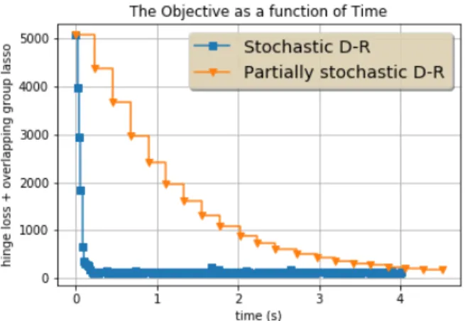
This strategy is compared with a partially stochastic Dou-glas Rachford algorithm, deterministic in the regulariza-tion G, where the fast subroutine Fog-Lasso [21] is used to compute the proximity operator of the regularization G. At each iteration n, the user is provided with (ξn, ηn). Then,
a Douglas Rachford step is done, involving the compu-tation of the proximity operators of the functions G and fn : x 7→ h(ηnhx, ξni). Figure 1 demonstrates the advantage
of treating the regularization term in a stochastic way. In Figure 1 "Stochastic D-R" denotes the stochastic Dou-glas Rachford algorithm and "Partially stochastic D-R" de-notes the partially stochastic Douglas Rachford where the su-broutine FoG-Lasso [21] is used at each iteration to compute
Fig. 1. The objective function F + G as a function of time in seconds for each algorithm
Fig. 2. Histogram of the Initialization and the last iterates of the Stochastic D-R (S. D-R) and the partially stochastic D-R (Part. S. D-R)
the true proximity operator of the regularization G. Figure 2 shows the appearance of the first and the last iterates. Even if a best performing procedure [21] is used to compute proxγG,
we observe on Figure 1 that Stochastic D-R takes advantage of being a stochastic method. This advantage is known to be twofold ([22]). First, the iteration complexity of Stochastic D-R is moderate because proxγG is never computed. Then, Stochastic D-R is faster than its partially deterministic coun-terpart which uses Fog-Lasso [21] as a subroutine, especially in the first iterations of the algorithms. Moreover, Stochastic D-R seems to perform globally better. This is because every proximity operators in Stochastic D-R can be efficiently com-puted ([23]). Contrary to the proximity operator of G [21], the proximity operator of gnis easily computable. The proximity
operator of fnis easily computable as well.3
3. Even if h(x) = log(1+exp(−x)) (logistic regression), the proximity operator of fnis easily computable, see [2].
6. REFERENCES
[1] S. Boyd, N. Parikh, E. Chu, B. Peleato, and J. Eckstein, “Distributed optimization and statistical learning via the alternating direction method of multipliers,” Founda-tions and Trends in Machine Learning, vol. 3, no. 1,R
pp. 1–122, 2011.
[2] G. Chierchia, A. Cherni, E. Chouzenoux, and J.-C. Pes-quet, “Approche de douglas-rachford aléatoire par blocs appliquée à la régression logistique parcimonieuse,” in GRETSI, 2017.
[3] P.-L. Lions and B. Mercier, “Splitting algorithms for the sum of two nonlinear operators,” SIAM J. Numer. Anal., vol. 16, no. 6, pp. 964–979, 1979.
[4] J. Eckstein and D. P. Bertsekas, “On the dou-glas—rachford splitting method and the proximal point algorithm for maximal monotone operators,” Mathema-tical Programming, vol. 55, no. 1, pp. 293–318, 1992. [5] P. Bianchi and W. Hachem, “Dynamical behavior of a
stochastic Forward-Backward algorithm using random monotone operators,” ArXiv e-prints, 1508.02845, Aug. 2015, To be published in J. Optim. Theory Appl. [6] P. Bianchi, W. Hachem, and A. Salim, “A
constant step Forward-Backward algorithm involving random maximal monotone operators,” arXiv preprint arXiv :1702.04144, 2017.
[7] A. Salim, P. Bianchi, and W. Hachem, “Snake : a sto-chastic proximal gradient algorithm for regularized pro-blems over large graphs,” in preparation, 2017.
[8] Z. Shi and R. Liu, “Online and stochastic douglas-rachford splitting method for large scale machine lear-ning,” arXiv preprint arXiv :1308.4757, 2013.
[9] A. Chambolle, M. J Ehrhardt, P. Richtárik, and C.-B. Schönlieb, “Stochastic primdual hybrid gradient al-gorithm with arbitrary sampling and imaging applica-tion,” arXiv preprint arXiv :1706.04957, 2017.
[10] L. Rosasco, S. Villa, and B.-C. Vu, “Stochas-tic inertial primal-dual algorithms,” arXiv preprint arXiv :1507.00852, 2015.
[11] P.-.L Combettes and J.-C. Pesquet, “Stochastic forward-backward and primal-dual approximation algorithms with application to online image restoration,” in Si-gnal Processing Conference (EUSIPCO), 2016 24th Eu-ropean. IEEE, 2016, pp. 1813–1817.
[12] R. Mourya, P. Bianchi, A. Salim, and C. Richard, “An adaptive distributed asynchronous algorithm with appli-cation to target localization,” in CAMSAP, 2017. [13] H. H. Bauschke and J. M. Borwein, “On projection
algo-rithms for solving convex feasibility problems,” SIAM review, vol. 38, no. 3, pp. 367–426, 1996.
[14] R. T. Rockafellar and R. J.-B. Wets, Variational analy-sis, vol. 317 of Grundlehren der Mathematischen Wis-senschaften [Fundamental Principles of Mathematical Sciences], Springer-Verlag, Berlin, 1998.
[15] A. Salim, P. Bianchi, and W. Hachem, “A stochas-tic douglas-rachford algorithm with constant step size,” Tech. Rep., see https ://adil-salim.github.io/Research, 2017.
[16] H. J. Kushner and G. G. Yin, Stochastic approxima-tion and recursive algorithms and applicaapproxima-tions, vol. 35 of Applications of Mathematics (New York), Springer-Verlag, New York, second edition, 2003, Stochastic Mo-delling and Applied Probability.
[17] H. Brézis, Opérateurs maximaux monotones et semi-groupes de contractions dans les espaces de Hilbert, North-Holland mathematics studies. Elsevier Science, Burlington, MA, 1973.
[18] P.-L. Combettes and J.-C. Pesquet, “Stochastic quasi-fejér block-coordinate fixed point iterations with ran-dom sweeping,” SIAM Journal on Optimization, vol. 25, no. 2, pp. 1221–1248, 2015.
[19] J.-C. Fort and G. Pagès, “Asymptotic behavior of a Mar-kovian stochastic algorithm with constant step,” SIAM J. Control Optim., vol. 37, no. 5, pp. 1456–1482 (elec-tronic), 1999.
[20] P. Bianchi, W. Hachem, and A. Salim, “Asymptotics of constant step stochastic approximations involving diffe-rential inclusions,” arXiv preprint arXiv :1612.03831, 2016.
[21] L. Yuan, J. Liu, and J. Ye, “Efficient methods for over-lapping group lasso,” in Advances in NIPS, 2011, pp. 352–360.
[22] L. Bottou, F. E Curtis, and J. Nocedal, “Optimization methods for large-scale machine learning,” arXiv pre-print arXiv :1606.04838, 2016.
[23] H. H. Bauschke and P. L. Combettes, Convex analysis and monotone operator theory in Hilbert spaces, CMS Books in Mathematics/Ouvrages de Mathématiques de la SMC. Springer, New York, 2011.