Cuspidal and Noncuspidal Robot Manipulators

(1)

HAL Id: hal-00454562

https://hal.archives-ouvertes.fr/hal-00454562

Submitted on 8 Feb 2010

HAL is a multi-disciplinary open access

archive for the deposit and dissemination of sci-entific research documents, whether they are pub-lished or not. The documents may come from teaching and research institutions in France or abroad, or from public or private research centers.

L’archive ouverte pluridisciplinaire HAL, est destinée au dépôt et à la diffusion de documents scientifiques de niveau recherche, publiés ou non, émanant des établissements d’enseignement et de recherche français ou étrangers, des laboratoires publics ou privés.

Philippe Wenger

To cite this version:

Philippe Wenger. Cuspidal and Noncuspidal Robot Manipulators. Robotica, Cambridge University Press, 2007, 25 (6), pp.717-724. �hal-00454562�

(2)

Final version Submitted to special issue “Geometry in Robotics and Sensing” of ROBOTICA 08/02/10

Cuspidal and Noncuspidal Robot Manipulators

Philippe Wenger

Institut de Recherche en Communications et Cybernétique de Nantes 1, rue de la Noë, 44321 Nantes, France

Email: Philippe.Wenger@irccyn.ec-nantes.fr

Abstract

This article synthezises the most important results on the kinematics of cuspidal manipulators i.e. nonredundant manipulators that can change posture without meeting a singularity. The characteristic surfaces, the uniqueness domains and the regions of feasible paths in the workspace are defined. Then, several sufficient geometric conditions for a manipulator to be noncuspidal are enumerated and a general necessary and sufficient condition for a manipulator to be cuspidal is provided. An explicit DH-parameter-based condition for an orthogonal manipulator to be cuspidal is derived. The full classification of 3R orthogonal manipulators is provided and all types of cuspidal and noncuspidal orthogonal manipulators are enumerated. Finally, some facts about cuspidal and noncuspidal 6R manipulators are reported.

Keywords: Cuspidal manipulator, Singularity, Posture, Workspace, Cusp Point, Classification.

1 Introduction

A cuspidal manipulator is a nonredundant manipulator that can change its posture (a posture is associated with an inverse kinematic solution) without meeting a singularity. Today, most industrial 6R manipulators are of the PUMA type, which is noncuspidal. Indeed, a Puma robot cannot avoid the fully extended arm configuration when moving from the “elbow up” to the “elbow down”

(3)

posture. Modification in the link arrangement is very likely to result in a cuspidal manipulator. In 1998, ABB-Robotics launched the IRB 6400C, a new manipulator specially designed for the car industry to minimize the swept volume. The only difference from the Puma was the permutation of the first two link axes, resulting in a manipulator with all its joint axes orthogonal. Commercialization of the IRB 6400C was finally stopped one year later. Informal interviews with robot customers at that time revealed difficulties in planning offline trajectories using Robotic-CAD systems for this robot. In fact it turns out that the IRB 6400C robot is cuspidal. We will come back to this robot in section 5.

It has long been believed that any manipulator always encounters a singularity during a change of posture1. The nonsingular change of posture was first pointed out in 1988 in two separate works. Parenti-Castelli and Innocenti exhibited a nonsingular posture changing trajectory for two different 6R cuspidal manipulators using numerical experiments2 while Burdick provided several examples of cuspidal 3R manipulators and some general results about which manipulators should be cuspidal3. Maybe because of the scepticism of the research community at that time, this feature has been ignored for several years and no further research work was provided before 1992, when the nonsingular posture-changing ability was confirmed and more formally analyzed4. As few authors have investigated this phenomenon since then, it took a long time before the research community recognized the nonsingular posture-changing ability. The problem of planning non-singular changing posture trajectories for general 3R manipulators was addressed by Tsai and Kholi in 19935. At the very end of his work, Smith suggested that a non-singular posture changing trajectory should encircle a cusp point in the workspace6. Burdick provided a list of conditions on the DH-parameters for a manipulator to be noncuspidal7. This list includes simplifying geometric conditions such as parallel and intersecting joint axes. Later, Wenger provided other conditions that are not intuitive8. A general, necessary and sufficient condition for a 3-DOF manipulator to be cuspidal was first established by El Omri and Wenger9 in 1995, namely, the existence of at least

(4)

one point in the workspace where the inverse kinematics admits three equal solutions. The word “cuspidal manipulator” was defined in accordance to this condition because a point with three equal inverse kinematic solution forms a cusp in a cross section of the workspace7,10. The different possible posture-changing motions for 3-DOF manipulators were analyzed by Wenger and El Omri11. The categorization of all generic 3R manipulators was established using homotopy classes, which made it possible to show that the space of 3R manipulators is mostly composed of cuspidal ones12. A procedure to take into account the cuspidality property in the design process of new manipulators was provided13. More recently, Corvez and Rouillier attempted the classification of 3R manipulators with orthogonal joints14. Five surfaces were found to divide the manipulator parameter space into cells with constant number of cusp points. The equations of these surfaces were derived as polynomials in the DH-parameters using Groebner Bases. A physical interpretation of this theoretical work was conducted by Baili et al15 who pointed out the existence of extraneous surface equations and took into account additional features in the classification like genericity16 and the number of aspects. The complete classification of orthogonal 3R manipulators was established for the first time in 2004 on the basis of the number of cusps and nodes in the workspace cross section17, 18. A general formalism for the kinematic analysis of cuspidal manipulators was provided and the maximal sets of feasible paths in the workspace were defined19.

The purpose of this work is to synthesize the most important results on the kinematics of cuspidal manipulators i.e. nonredundant manipulators that can change posture without meeting a singularity. The rest of this article is organized as follows. Section 2 introduces an illustrative cuspidal manipulator and recalls some facts about singularities and aspects. Section 3 defines the characteristic surfaces, the uniqueness domains and the regions of feasible paths in the workspace. Section 4 is devoted to the classification and enumeration of cuspidal and noncuspidal manipulators. The last section addresses the case of 6R manipulators.

(5)

2 Preliminaries

2.1 Illustrative Manipulator

A typical 3R cuspidal manipulator is used as illustrative example in this section. A 3R cuspidal manipulator should not have parallel or intersecting joint axes to be cuspidal7, 8. The geometric parameters of this manipulator, known as DH-parameters, are taken as 1=-/2, 2=/2, a1=1,

a2=2, a3=1.5, d1=0, d2=1, d3=0. This manipulator with mutually orthogonal joint axes (henceforth referred to as an orthogonal manipulator) has a rather simple geometry and is a good representative example11, 13. The three joint variables are referred to as 1, 2 and 3, respectively. Fig. 1 shows the

kinematic architecture of the manipulator in its zero configuration, i.e. 1 = 2 = 3 = 0. This

manipulator can be regarded as the regional structure of a 6R robot with a spherical wrist. The position of the end-tip is defined by the three Cartesian coordinates px, py and pz of the operation point P with respect to a reference frame (O, X, Y, Z) attached to the manipulator base (Fig. 1).

z _y O x P ₁ 2 3 a1 d2 a3 a2

.

S1 S2 A sp ect A1 A sp ect A2 3 [rad ] 3 2 1 0 -1 -2 -3 -3 -2 -1 0 2[rad ] 1 2 3

Fig. 1. A cuspidal 3R manipulator. Fig. 2. Aspects of the cuspidal manipulator.

2.2 Singularities and aspects

The singularities of a manipulator play an important role in its global kinematic properties3-7, 1-22. The singularities of a 3R manipulator can be determined using a recursive appoach23 or with det(J),

(6)

the determinant of the Jacobian matrix (px,py,pz)/(1,2,3)7,8,12,15. This determinant can be

derived automatically with symbolic softwares such as SYMORO24. For the illustrative manipulator, det(J) takes the following factored form,

2 3 3 2 3 2 3 2 3 1

det( )J  (a c a )(c (s a -c d ) s a ) (1)

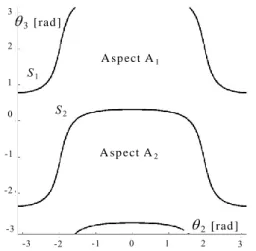
where ci=cos(i) and si=sin(i). A singularity occurs when det(J)=0. Since the singularities are independent of 1, the contour plot of det(J)=0 can be displayed in  2 , 3  . For the

illustrative manipulator a2>a3 and the first factor of det(J) cannot vanish (examples with a2<a3 will

be shown in Fig. 11 in section 4.3). Fig. 2 shows that the singularities form two closed surfaces S1

and S2 in the joint space. If the manipulator has no joint limits, S1 and S2 divide the joint space into

two singularity-free open, connected sets A1 and A2 called c-sheets3 or aspects1. We use the term

„aspect‟ because it is also used for manipulators with limited joints whereas c-sheets were defined for manipulators with unlimited joints only.

2.3 Singularities and workspace

The workspace of general 3R manipulators has been widely studied since the seventies1,3-8, 17-22,

25-36

. The determination of the workspace boundaries, the size and shape of the workspace, the existence of holes and voids, accessibility inside the workspace (i.e. the number of inverse kinematic solutions) are some of the main features that have been explored. The singularities can be displayed in Cartesian space where they define boundaries. Thanks to their symmetry about the first joint axis, a representation in a half cross-section of the workspace is sufficient (Fig. 3). As in the joint space, the singularities also form two disjoint curves in the workspace. These two curves define the internal boundary WS1 and the external boundary WS2, respectively. If f denotes the

kinematic map, then WS1=f(S1) and WS2=f(S2). The separating and sorting of these boundary curves

(7)

two inverse kinematic solutions (the outer region) and one region with four inverse kinematic solutions (the inner region, Fig. 3). Each point on the internal boundary has three distinct inverse kinematic solutions, one of which is a double solution. At each cusp point, there are only two distinct inverse kinematic solutions, one of them being a triple solution4. The external boundary surface is composed of two adjacent arcs that meet on axis Z. There is only one inverse kinematic solution on the external boundary, which is a double solution. There are an infinite number of inverse kinematic solutions at the two connecting points on axis Z (because 1 can take on any

value without altering the position of the end-tip).

O uter region (2 IK S ) Internal boundary W S1= B S1B S2B S3B S4 (3 IK S ) Inner R egion : (4 IK S ) E xternal boundary W S₂(1 IK S ) C usp point (2 IK S ) B S2 B S1 B S3 B S4 z [m ] 2 2 x y  



[m ]

Fig. 3. Singularity locus in workspace. Number of distinct inverse kinematic solutions (IKS) in each region and on each boundary is indicated.

(8)

2.4 A nonsingular posture changing trajectory

For the illustrative manipulator, solving the inverse kinematics at px=2.5, py=0, pz=0.5 yields four solutions given (in radians) by q(1)=[-1.8 -2.8 1.9]t, q(2)=[-0.9 -0.7 2.5]t, q(3)=[-2.9 -3 -0.2]t and

q(4)=[0.2 –0.3 –1.9]t. It is apparent from fig. 4 that q(2) and q(3) (resp. q(1) and q(4) ) lie in the same aspect A1 (resp. A2), which means that these two solutions are not separated by a singularity. It is

then possible to link q(2) and q(3) by a nonsingular straight line trajectory. When projected in the workspace cross section, this trajectory traces a loop path that encompasses a cusp point (Fig. 4). In fact it has been shown that a nonsingular posture-changing trajectory always encompasses a cusp point in the workspace4-6, 9, 11.

S1 A sp e c t A2 A sp e c t A1 q(1 ) q(4 ) q(3 ) q(2 ) ₃[ra d ] ₂[ra d ] W A1 = W A2 P z [m ]  [m ]

Fig. 4. A point with two inverse kinematic solutions in each aspect. A nonsingular posture changing trajectory and the resulting path in workspace section are displayed.

On the other hand, there is only one inverse kinematic solution per aspect for any point in the outer region. The two aspects A1 and A2 map onto the same set WA1=WA2 in the workspace, with the

same internal and external boundaries as in Fig. 4. In WA1 or in WA2, there are only two solutions

(9)

3 Formalism for the kinematic analysis of cuspidal manipulators

In this section, the notion of characteristic surfaces and uniqueness domains is introduced. Not every motion is feasible in the workspace of a cuspidal manipulator, even without joint limits. It is shown that the regions of feasible motions in the workspace are defined as the image of the uniqueness domains through the kinematic map. This holds for any nonredundant manipulator with or without joint limits.

3.1 Characteristic surfaces

Since the singular surfaces in the joint space do not separate all the inverse kinematic solutions, new separating surfaces should exist. The set obtained by calculating the nonsingular inverse kinematic solutions for all points on an internal boundary forms a set of nonsingular surfaces in each aspect. We call these surfaces the characteristic surfaces. A set of characteristic surfaces is associated with one aspect and it was proved that they separate the inverse kinematic solutions in each aspect17. A general definition of the characteristic surfaces can be set as follows, which stands for any nonredundant manipulator with or without joint limits. Let A *_i be the boundary of aspect Ai. The characteristic surfaces {CSi} associated with Ai are :

1

i i

{C S_i} f ( f(A *))A (2)

where f(A *_i ) is the image of A *_i under the forward kinematic map and f-1(f(A *_i )) = {q / f(q)  f(A *i )}. Note that since an aspect is defined as an open set, Ai does not contain its boundary i.e.

i

i*

A A  thus {CSi} might be empty (this is so for noncuspidal manipulators).

Note that the characteristic surfaces are slightly different from the pseudo-singular surfaces defined by Tsai5 and Miko35 as f-1(f(A *i )). The pseudo-singular surfaces were defined for 3R manipulators

(10)

manipulator with more than two aspects, the pseudo-singular surfaces generate “spurious” surfaces that do not separate the inverse kinematics solutions. In fact, the pseudo-singular surfaces and the characteristic surfaces are equivalent for manipulators with unlimited joints and having only two aspects. Fig. 5 shows the two characteristic surfaces {CS1} and {CS2} for the illustrative

manipulator. S in gu lar su rfaces C h aracteristic S u rfaces {C S1} C h aracteristic S u rfaces {C S2} 3[rad ] 2[rad ]

Fig. 5. Singular and characteristic surfaces.

The characteristic surfaces are independent of 1 when 1 is unlimited. Because the general

definition (2) is not algebraic in nature, it is difficult to derive an algebraic expression of {CSi} that would be easy to handle. A scanning process can be used to plot the characteristic surfaces19.

The characteristic surfaces induce a partition of each aspect into open sets that we call reduced

aspects. Also, the internal boundaries induce a partition of the workspace into regions and each

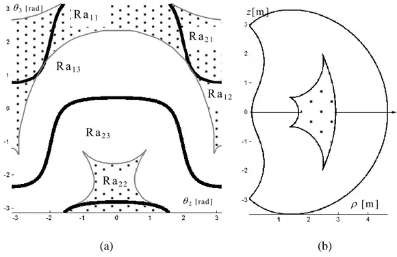
such region is associated with several reduced aspects. For the illustrative manipulator of Fig. 1, the inner region is associated with the four reduced aspects Ra11, Ra12, Ra21 and Ra22 (in gray in Fig. 6).

(11)

The first two, Ra11 and Ra12, are in A1, whereas Ra21 and Ra22 are in A2. The outer region is

associated with the two reduced aspects Ra13 and Ra23 that belong to A1 and A2, respectively.

A1 A2 R a22 R a13 R a23 R a11 R a21 R a12 3[rad ] 2[rad ] R a22 z[m ]  [m ] (a) (b)

Fig. 6. Correspondence between the reduced aspects (a) and the regions (b).

3.2 Uniqueness domains

Fig. 6 shows that each aspect is made of three reduced aspects, two of them being associated with the same region in the workspace (Ra11 and Ra12 for aspect A1). If we remove one of these two

reduced aspects and its boundary from the aspect, the remaining domain is a uniqueness domain. Thus, there is still a unique inverse kinematic solution in the domain defined by Qu1=A1_.C(Ra12) as

well as in Qu2= A1_.C(Ra11) (_. means the difference between sets, C(R) means the closure of R). In

the same way, Qu3=A2_.C(Ra22) and Qu4=A2_.C(Ra21) are still uniqueness domains. Fig. 7 shows

(12)

Final version Submitted to special issue “Geometry in Robotics and Sensing” of ROBOTICA 08/02/10 A1 Q u1 3[rad ] 2 [rad ] Q u2 3[rad ] 2[rad ] A2 C S2 Q u3 3 [rad ] 2[rad ] Q u4 3 [rad ] 2[rad ]

Fig. 7. Four maximal uniqueness domains for the illustrative manipulator of Fig. 1.

3.3 Regions of feasible paths in the workspace

For a noncuspidal manipulator, the regions of feasible paths in the workspace are the image of the aspects1. This is not true for a cuspidal manipulator because the aspects are not the uniqueness domains. The regions of feasible paths in the workspace must be defined by the uniqueness domains. Figure 8 shows the four regions of feasible paths, which are the images of the uniqueness domains in the workspace. It is important to note that Wf1, Wf2, Wf3 and Wf4 define regions where

(13)

any arbitrary path is feasible but they do not include all feasible paths. In effect, it is possible to

define a feasible path that undergoes a nonsingular change of posture in, say, aspect A1 like in Fig.

4. In this case, the path will start in Wf1 and stop in Wf2.

[m] z[m] [ m ] z [ m ] Wf1 = f(Qu1) Wf2 = f(Qu2) [ m ] z [ m ] [ m ] z [ m ] Wf3 = f(Qu3) Wf4 = f(Qu4)

Fig. 8. Regions of feasible paths.

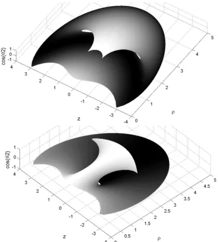
To get the full model of feasible paths in WA1, Wf1 and Wf2 must be properly “glued” together,

which can be realized by plotting the surface (, z, cos((2)) for A119. From a mathematical point of

(14)

provides the full model of feasible paths in WA2 (Fig. 9). This model helps better understand the

nonsingular posture changing phenomenon and the loop path shown in Fig. 4.

Fig. 9. Full model for the feasible paths in WA1 (above) and WA2 (below).

The uniqueness domains and the regions of feasible paths of any 3R manipulators can be got quite simply when the singular curves and the characteristic surfaces are given19. The regions of feasible paths are useful to assess the global performances of a manipulator and to compare several manipulator designs. These regions can also be used to verify the feasibility of a path without analyzing the root equality of the inverse kinematic polynomial on the boundaries. In effect, since each region of feasible paths is associated with one inverse kinematic solution, these regions indicate which internal surfaces can be crossed, according to the inverse kinematic solution used to follow the path19.

(15)

The characteristic surfaces, the uniqueness domains and the regions of feasible paths can be calculated in the same way for 3R manipulators with joint limits on their last two axes19. When joint 1 is also limited, it is no longer possible to build 2D sections. Such manipulators were investigated by El Omri and their uniqueness domains and regions of feasible paths were built using octrees38.

4 ENUMERATION

OF

CUSPIDAL

MANIPULATORS

AND

CLASSIFICATION

4.1 Simplifying geometric conditions

Because of the more complex behavior of a cuspidal robot and because of the difficulty in modeling its kinematic properties, industrial robots should be designed noncuspidal rather than cuspidal. Thus, before designing an innovative kinematic architecture, robot manufacturers should have guidelines such as design rules to help them. Why a manipulator with a given geometry is cuspidal has long been a very intriguing question. It is worth noting that this question remains not completely solved. One of the pioneer contributors to this problem was J. Burdick, who observed that under simplifying geometric conditions such as intersecting or parallel joint axes, a 3R manipulator was noncuspidal7. Other simplifying conditions were exhibited later7 as a direct consequence of the necessary and sufficient condition recalled in next section. Finally, six geometric conditions were found to define noncuspidal 3R manipulators:

1/ first two joint axes are parallel (sin(1)=0),

2/ last two joint axes are parallel (sin(2)=0),

3/ first two joint axes intersect (a1=0),

(16)

5/ first two joint axes are orthogonal, all joint offsets are zero (cos(1)=0, d2=0, d3=0),

6/ joint axes are mutually orthogonal, first joint offset vanishes (cos(1)=cos(2)=0, d2=0).

These conditions also hold for 6R manipulators with spherical wrist because the singularity analysis of the wrist can be decoupled from those of the regional structure. It is worth noting that conditions 2/ and 3/ are encountered in most industrial 6R manipulators. However, the last two conditions (5/ and 6/) are unusual.

Analogous conditions exist also for manipulators with prismatic joints39.

4.2 Necessary and sufficient condition for a manipulator to be cuspidal

Burdick conjectured that, on the other hand, 3R manipulators with “general” geometry should be cuspidal6. But it was shown later that the correlation between cuspidal manipulators and general manipulators was not clear8. For example, the orthogonal manipulator shown in Fig. 1 is cuspidal but it is no longer cuspidal when a3 is set to 0.5m instead of 1.5m (with the same values for the remaining DH-parameters). In both cases the manipulators are not of “general geometry” in the sense that the last joint offset is equal to zero and the joint axes are mutually orthogonal. An important step towards the characterization of cuspidal manipulators was established in 1995 when a general necessary and sufficient condition for a manipulator to be cuspidal was provided. This condition states that a manipulator is cuspidal if and only if its inverse kinematics admits a triple solution9 (i.e. a point where three inverse kinematic solutions coincide). In the cross section of the workspace of a 3R manipulator, a point with three equal inverse kinematic solutions is a cusp point (see the four cusp points in Fig. 3). A direct consequence of this condition is that for a manipulator to be cuspidal, the degree of its inverse kinematics polynomial must be greater than 2. Hence, any

quadratic manipulator (i.e. whose inverse kinematic polynomial can be reduced to a quadratics) is

noncuspidal. All six noncuspidal manipulator types enumerated in the preceding section are quadratic38. Also, any 3-DOF manipulator (or 6-DOF with wrist) with at least two prismatic joints

(17)

are always quadratic40 and thus cannot be cuspidal. But it took eight years before this condition could be exploited to derive more general conditions on the DH-parameters14. The exploitation of the necessary and sufficient condition is recalled hereafter.

4.3 Classification of 3R orthogonal manipulators

For a 3R manipulator, the existence of cusps can be determined from its fourth-degree inverse kinematic polynomial P(t) in ttan3/ 2 whose coefficients are function of the DH-parameters

and of the variables 2 2

R x  y and 2

Z z (see reference30 for more details on the derivation and properties of this polynomial). The condition for P(t) to have three equal roots can be set as follows: 2 3 1 2 2 2 3 1 2 2 2 2 3 1 2 2 2 ( , , , , , , , ) 0 ( , , , , , , , ) 0 ( , , , , , , , ) 0 P t a a d R Z P t a a d R Z t P t a a d R Z t                       (3)

The three variables t, R and Z must be eliminated to obtain a condition on the DH-parameters. Deriving a symbolic solution of (3) in the general case is not reasonable and has still not been attempted. On the other hand, the study of the particular case 1=/2, 2=/2 (orthogonal manipulators) is interesting because this case is more tractable (although still very complex) and the family of orthogonal manipulators is rich enough to define alternative designs with relatively simple geometries that could find potential applications in industry.

Rather than simply distinguishing between cuspidal and noncuspidal orthogonal manipulators, it is more interesting to classify the family of orthogonal manipulators as function of their number of cusp points. Indeed, the number of cusps provides more information about the topology of the singular curves in the workspace and, as a result, about the global properties of the manipulator such as the existence of voids and of 4-solution regions6,17,20,30. To do this classification, it is

(18)

appropriate to search for the conditions under which the number of real solutions of system (3) changes41. By doing so, a set of bifurcating surfaces is defined in the parameter space of orthogonal manipulators where the number of cusps changes. These bifurcating surfaces divide the parameter space into domains where all manipulators have the same number of cusp points. The bifurcating surfaces can be regarded as sets of transition manipulators. The algebra involved in system (3) is too complex to be handled by commercial computer algebra tools. Corvez and Rouillier14 resorted to sophisticated computer algebra tools to solve system (3) by first considering the more particular case d3=0 (no offset along the last joint axis like the robot shown in fig. 1). They used Groebner

Bases and Cylindrical Algebraic Decomposition41,42 to find the equations of the bifurcating surfaces and the number of domains generated by these surfaces. They obtained 5 distinct surface equations, which were shown to define 105 domains in the parameter space. A kinematic interpretation of this theoretical work was conducted by Baili et al15 : the authors analyzed global kinematic properties of one representative manipulator in each domain. Only 5 different cases were found to exist. In fact, several surface equations obtained by Corvez and Rouillier were extraneous solutions. Finally, the true bifurcating surfaces were shown to take on the following explicit form15:

C1 : 2 2 2 2 2 2 2 2 2 2 2 3 2 2 ( ) ( ) 1 ( ) 2 a d a d a a d A B       (4) C2 : 3 2 2 1 a a A a   (5) C3 : 3 2 2 2 a n d 1 1 a a B a a    (6) C4 : 2 3 2 2 a n d 1 1 a a B a a    (7) where 2 2 2 2 2 2 2 2 ( 1) and ( 1) A a  d B a  d (8)

(19)

Note that the above equations assume d3=0. Moreover, a1 was set to 1 without loss of generality in order to handle only three independent parameters. These four surfaces divide the parameter space into 5 domains with 0, 2 or 4 cusps. Fig. 10 shows the plots of the surfaces in a section (a2, a3) of

the parameter space for d2=1. Plotting sections for different values of d2 changes the size of each

region but the general pattern does not change and the number of cells remains the same. There are two domains of noncuspidal manipulators (domains 1 and 5), two domains of manipulators with four cusps (domains 2 and 4) and one domain of manipulators with two cusps.

a3

a2

Fig. 10. Plots of the bifurcating surfaces in a section (a2, a3) of the parameter space for d2=1.

The partition of the parameter space and the equations of the bifurcating surfaces allow us to define an explicit necessary and sufficient condition for an orthogonal manipulator with no offset along its last joint axis to be cuspidal. In effect, figure 10 shows that a manipulator is cuspidal if and only if it belongs to domains 2, 3 or 4. Thus, an orthogonal manipulator with no offset along its last joint axis is cuspidal if and only if:

2 2 2 2 2 2 2 2 2 2 1 2 2 3 2 2 ₂ ₂ 2 2 2 1 2 2 1 2 ( ) ( ) 1 ( ) 2 ₍ ₎ ₍ ₎ a d a a d a a d a a d a a d           (9) and _a _a _{or (}_a  _a _{a n d} _a  a2 ₍_a _a ₎2_d 2₎  (10)

(20)

Note that parameter a1 was no longer set equal to 1 in order to show better the influence of all

parameters. Fig. 11 shows the cross sections of the workspace and the singular curves in the joint space, for one representative manipulator in each domain of the partition. The number of inverse kinematic solutions in each region of the workspace is indicated. Fig. 11 shows that manipulators in domain 1 have only two inverse kinematics solutions. Also, they have a void in their workspace and they are noncuspidal. In fact, it can be shown that all other manipulators have 4 inverse kinematic solutions and that Eq. (9) is a necessary and sufficient condition for an orthogonal manipulator with d3=0 to have four inverse kinematic solutions20. The other noncuspidal

manipulators are in domain 5. They have a region with 4 inverse kinematic solutions and no void.

4 2

Domain 1 (a2=0.7, a3=0.3, d2=0.2) Domain 2 (a2=2, a3=1.5, d2=1)

Domain 3 (a2=3, a3=4, d2=3) Domain 4 (a2=2, a3=6, d2=1)

(21)

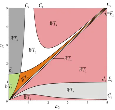
Each domain of the parameter space can be further classified by taking into account the number of nodes, i.e., the number of intersection points on the workspace boundaries17. There is one node in the workspace of the illustrative manipulator of domain 3 (fig. 11) but two more nodes may arise when the internal boundary goes outside the external one (as displayed in Fig. 13, WT6). Two more

surface equations E1=1( )

2 AB , E2=a2 and E3= 1

( )

2 AB (A and B are defined as in (8)) appear when the number of nodes is considered and the parameter space is divided into 9 cells, each one being associated with a particular workspace topology WTi. This new partition is shown in a section (a2, a3) of the parameter space for d2=1 (Fig. 12).

7

a

3

a

2

WT1: 0 cusp, 0 node, WT2: 4 cusps, 2 nodes, WT3: 4 cusps, 0 node

WT4: : 4 cusps, 2 nodes, WT5: 2 cusps, 1 node, WT6: 2 cusps, 3 nodes,

WT7: 4 cusps, 4 nodes, WT8: 0 cusp, 0 node, WT9: 0 cusp, 2 nodes

Fig. 12. Partition of the parameter space according to the number of cusps and nodes.

Plots of the separating curves in sections for different values of d2 show that they deform smoothly

with the same intersections when d2 varies. The areas of WT1, WT2, WT7 and WT9 increase when r2

(22)

no node (this domain is referred to as WT1), all manipulators in domains 4 have four nodes (WT7).

Manipulators in domains 2 and 5 may have no nodes (WT3 and WT8, respectively) or two nodes

(WT2 and WT9, respectively) and manipulators in domain 3 may have one or three nodes (WT5 and WT6, respectively).

The classification with nodes makes it possible to identify all the orthogonal manipulators that have a void in their workspace. In effect, all such manipulators are in domains WT1 and WT2.

Fig. 13 shows the cross sections of the workspace and the singular curves in the joint space, for one representative manipulator in WT2, WT4, WT6 and WT9. The other representative manipulators

appear in fig. 11. The two horizontal singular lines that appear in the joint space of the manipulators in WT4 and WT6 generate isolated points in the workspace cross section as shown by

arrows in Fig. 12.

Domain 2, WT2, (a2=1.5, a3=0.7, d2=0.5) Domain 2, WT4, (a2=3, a3=4, d2=9)

Domain 3, WT6, (a2=3, a3=4, d2=2) Domain 5, WT9, (a2=0.5, a3=1.3, d2=0.2)

(23)

The preceding classification stands for orthogonal manipulators with no offset along their last joint axis (d3=0). For manipulators with nonzero offsets, it is possible to solve system (3) as above but

the resulting separating surface equations get very complicated and the parameter space is four-dimensional18. The complete classification for general 3R orthogonal manipulators was conducted in Baili‟s PhD thesis43

. The classification shows that manipulators may have 0, 2, 4, 6 or 8 cusps. The equation of one of the bifurcating surfaces between domains with different number of cusps is a 12th-degree polynomial in the square of the DH-parameters and contains 536 monomials. It is interesting to remark that when d3 is set to zero, this equation simplifies considerably and factors.

Equating the three factors to zero gives exactly the three equations (5), (6) and (7).

For small values of d3, the partition sections look like those in Fig. 12 but the subspace WT4 does

not exist any more. It is replaced by two adjacent subspaces with 6 and 8 cusps, located near a3=a2.

For high values of d3, the partition gets very complicated with not less than 22 distinct topologies.

Figure 14 shows an example of a workspace topology with 8 cusps and 4 nodes. The zoomed view shows the creation of a pair of cusps, a pattern known as a swallowtail44.

a1 = 1 , a2 = 0 .7, a3 = 0 .7,

d2 = 0 .3 , d3 = 0 .9

void

(24)

Note1: all results about the classification presented in this section assume that a1, a2, a3 and d2 are different from zero. In any other case, the manipulator is noncuspidal (this is because if one of these parameters is equal to zero, one of the simplifying conditions given in section 3.1 is satisfied). However the classification according to the number of nodes is still possible and was conducted recently by Zein et al45. The classification revealed interesting noncuspidal 3R orthogonal architectures with good workspace properties (workspace of regular shape, fully reachable with four inverse kinematic solutions and in which any path is feasible) that could find industrial applications.

Note2: the classification of 3-DOF manipulators with one prismatic joint can be attempted with the

same tools as for 3R manipulators. Because the kinematic equations are simpler when a prismatic joint is involved, the classification would be simpler.

5 Some facts about cuspidal 6R robots

The above classifications also hold for 6R manipulators with spherical wrist (i.e, with their last three joint axes intersecting at a common point) because the singularity analysis of the wrist can then be decoupled from that of the regional structure. In the introduction of this paper, we reported the story of the IRB 6400C robot. This robot, shown in Fig. 15, has a spherical wrist and its regional structure is an orthogonal 3R manipulator that can be shown to be cuspidal43. Note that the main objective of this new robot design was to save space and this is why its first joint axis is horizontal instead of vertical46. This was a good idea but at the time the engineers of ABB designed their new robot, the classification results were not published. It would be interesting to attempt a new design, keeping the orthogonal architecture with its first axis horizontal but tuning the length parameters in order that the robot falls in one of the interesting classes of noncuspidal orthogonal manipulators described by Zein et al45.

(25)

Fig. 15. The ABB IRB 6400C robot.

On the other hand, there is no general result about the enumeration of cuspidal 6–DOF manipulators with nonspherical wrist. One of the reasons is the difficulty in analyzing the singularities of general 6R robots, which depend on four joint variables instead of two in 3R robots. We think that 6R manipulators are very likely to be cuspidal, even if the simplifying geometric conditions listed in section 4.1 are satisfied. This is because the inverse kinematics of most 6-DOF manipulators with nonspherical wrist is a polynomial of degree higher than 4, which may admit triple roots. Further research work is required before stating more definitive results but several examples of simple 6R robots with nonspherical wrist exist. One of these robots is the GMF P150 shown in Fig. 16 used in the automotive industry for car painting (a similar version exists by COMAU). This robot is close to a PUMA robot, the only difference being the presence of a wrist offset. El Omri showed that without taking account the joint limits, this robot has 16 inverse kinematic solutions and only two aspects38. Thus, it is cuspidal. Another example is the ROBOX painting robot studied by M. Zoppi47 (Fig. 17). The kinematic architecture is very close to the GFM P150 but the wrist offset is not along the same wrist axis. This cuspidal robot has also 16 inverse kinematic solutions and only two aspects.

(26)

Fig. 16. The GMF P150 robot. Fig. 17. The ROBOX robot.

If the enumeration of 6-dof cuspidal and noncuspidal manipulators is far from being established, it is possible to enumerate a set of noncuspidal ones, namely, those whose inverse kinematics polynomial is a quadratics (because no cusp point exists in this case). Such manipulators were enumerated by Mavroidis and Roth in 199648.

6 Concluding remarks

This synthesis article on cuspidal manipulators can be summarized as follows.

Cuspidal manipulators, which were first discovered in 1988, have multiple inverse kinematic solutions (IKS) that are not separated by a singular surface. In the joint space, additional surfaces, called the characteristic surfaces, divide the aspects and separate the IKS. These surfaces are used to define new uniqueness domains and regions of feasible paths in the workspace. The definitions are general and stand for any serial, nonredundant manipulator with or without joint limits. For 3-DOF manipulators, it is possible to calculate and plot these characteristic surfaces, uniqueness domains and regions of feasible paths. If the first joint is revolute and unlimited, 2-dimensional plots are sufficient. Because there is no simple algebraic definition, these sets must be calculated

(27)

A 3R manipulator is noncuspidal as soon as its first two or last two joint axes are parallel or intersect, or if the three joint axes are mutually orthogonal and the first joint offset is equal to zero. But an orthogonal manipulator with its last joint offset equal to zero may be cuspidal.

A manipulator is cuspidal if and only if there is at least one point where three inverse kinematic solutions coincide. For a 3-DOF manipulator, this point appears as a cusp point in a cross section of the workspace. This necessary and sufficient condition for a manipulator to be cuspidal makes it possible to classify orthogonal manipulators as function of the number of cusps and nodes in the workspace. For orthogonal manipulators with no joint offset along their last axis, this classification enables one to derive explicit DH-parameter based necessary and sufficient conditions for a manipulator to be cuspidal, to have four inverse kinematic solutions or to have a void in its workspace. For general 3R orthogonal manipulators, the classification is much more complex and does not lend itself to explicit conditions.

Little research work has been conducted on 6R cuspidal manipulators. It appears that 6R robots with nonspherical wrist are very likely to be cuspidal, even if two joint axes intersect or are parallel. However, there is still much work to do before having definitive geometric conditions for general 6R robots. Resorting to some transversality theorems used by singularity theorists would help going further, providing that we remain in the generic case16,49. So the first step would be to enumerate all 6R generic manipulators.

The case of parallel manipulators has not been considered in this article. As first observed in 1998, a parallel manipulator may be cuspidal in the sense that it may change its assembly-mode without crossing a parallel-type singularity50, 51. As shown by R. McAree52 and explained in details by Zein53, to be cuspidal, a parallel manipulator should have 3 coincident assembly modes, which define a cusp point in a section of its joint space. Because the kinematic equations of a parallel manipulator are very complex, it seems very difficult to derive general geometric conditions for a parallel manipulator to be cuspidal. To the author‟s knowledge, the only available results pertain to

(28)

planar manipulators : to be cuspidal, a 3-DOF parallel planar manipulator with three RPR legs should not have similar platform and base triangles52, 54 but this is false if the legs are RRR instead of RPR55 (the underlined letter refers to the actuated joint).

Acknowledgment

Most of the classification work summarized in this article has been conducted in collaboration with IRMAR (Institute of Applied Mathematics of Rennes), INRIA (Research Institute of Informatics and Automatics), and LIP6 (Informatics Laboratory of Paris VI), in the frame of the national program MATHSTIC entitled “Cuspidal robots and triple roots” funded by C.N.R.S. (French Council of Scientific Research) and French Ministry of Education and Research.

References

[1] P. Borrel and A. Liegeois, "A study of manipulator inverse kinematic solutions with application to trajectory planning and workspace determination,", in Proc. IEEE Int. Conf. Rob. and Aut., pp 1180-1185, 1986.

[2] C.V. Parenti and C. Innocenti, "Position Analysis of Robot Manipulators : Regions and Sub-regions," in Proc. Int. Conf. on Advances in Robot Kinematics, pp 150-158, 1988.

[3] J. W Burdick, "Kinematic analysis and design of redundant manipulators," PhD Dissertation, Stanford, 1988.

[4] P. Wenger, “A new General Formalism for the Kinematic Analysis of all Non-Redundant Manipulators”, Proc. IEEE Int. Conf. on Rob. and Aut., pp 442-447, 1992.

[5] K.Y. Tsai and D. Kholi, "Trajectory planning in task space for general manipulators," ASME J. of Mech. Design, Vol. 115, p. 915-921, 1993.

(29)

[6] D.R. Smith and H. Lipkin, “Higher Order Singularities of Regional Manipulators”, IEEE International Conference on Robotics and Automation, Atlanta, U.S.A, 1993.

[7] J. W Burdick, "A classification of 3R regional manipulator singularities and geometries," Mechanisms and Machine Theory, Vol 30(1), pp 71-89, 1995.

[8] P. Wenger, "Design of cuspidal and noncuspidal manipulators," in Proc. IEEE Int. Conf. on Rob. and Aut., pp 2172-2177., 1997

[9] J. El Omri and P. Wenger : "How to recognize simply a nonsingular posture changing 3-DOF manipulator," Proc. 7th Int. Conf. on Advanced Robotics , p. 215-222, 1995.

[10] V.I. Arnold, Singularity Theory, Cambridge University Press, Cambridge, 1981.

[11] P. Wenger and J. El Omri, "Changing posture for cuspidal robots," in Proc. IEEE Int. Conf. on Rob. and Aut., pp 3173-3178, 1996.

[12] P. Wenger, "Classification of 3R positioning manipulators ," ASME Journal of Mechanical Design, Vol. 120(2), pp 327-332, 1998.

[13] P. Wenger, "Some guidelines for the kinematic design of new Manipulators," Mechanisms and Machine Theory, Vol 35(3), pp 437-449, 2000.

[14] S. Corvez and F. Rouillier, "Using computer algebra tools to classify serial manipulators," in Automated Deduction in Geometry, vol. 2930 of Lecture Notes in Computer Science, pp31-43, Springer, 2004.

[15] M. Baili, P. Wenger and D. Chablat, "Classification of one family of 3R positioning manipulators," in Proc. 11th Int. Conf. on Adv. Rob., 2003.

[16] D.K. Pai and M.C. Leu, "Genericity and Singularities of Robot Manipulators", IEEE Trans. on Rob. and Aut., Vol 8(5), pp 545-559, October 1991.

[17] M. Baili, P. Wenger and D. Chablat, "A Classification of 3R orthogonal manipulators by the Topology of their Workspace, " in Proc. IEEE Int. Conf. Rob. and Aut., 2004.

(30)

[18] P. Wenger, M. Baili and D. Chablat, “Workspace Classification of 3R orthogonal manipulators,” On Advances in Robot Kinematics, Kluwer Academic Publisher, pp. 219-228, 2004.

[19] P. Wenger, “Uniqueness domains and regions of feasible continuous paths for cuspidal manipulators,” IEEE Transactions on Robotics, Vol 20(4), August 2004.

[20] P. Wenger, P., D. Chablat and M. Baili, “A DH-parameter based condition for 3R orthogonal manipulators to have 4 distinct inverse kinematic solutions”, Journal of Mechanical Design, Vol. 127(1), pp 150-155, january 2005.

[21] F. Ranjbaran and J. Angeles, “On Positioning Singularities of 3-Revolute Robotic Manipulators”, Proc. 12th Symp. on Engineering Applications in Mechanics, pp 273-282, Montreal, CA, 1994.

[22] A. Urbanic and J. Lenarcic, “Kinematic Considerations on General 3R Manipulators”, Proc. 3rd Int. Workshop on Robotic in the Alpe-Adria, pp 293-298, Slovenia, 1994.

[23] J.W. Burdick, "A Recursive Method for Finding Revolute-Jointed Manipulator Singularities," ASME Journal of Mechanical Design, Vol. 117(1):55-63, 1995.

[24] W. Khalil and D. Creusot, “SYMORO+, a system for the modeling of robots”, Robotica, Vol. 15, No. 2, March, 1997.

[25] B. Roth, "Performance evaluation of manipulators from a kinematic viewpoint", Performance evaluation of programmable robots and manipulators, NBS Special Publication, 1975.

[26] A. Kumar and K.J. Waldron, “The workspace of a mechanical manipulator,” ASME Journal of Mechanical Design, Vol. 103., pp. 665-672, 1981.

[27] K.C. Gupta and B. Roth, “Design Considerations for Manipulator Workspaces,” ASME Journal of Mechanical Design, Vol. 104, pp. 704-711, 1982.

(31)

[28] D.C.H Yang and T.W. Lee, “On the workspace of mechanical manipulators,” ASME Journal of Mechanical Design, Vol. 105, pp. 62-69, 1983.

[29] F. Freudenstein and E.J.F. Primrose, “On the Analysis and Synthesis of the Workspace of a Three-Link, Turning-Pair Connected Robot Arm,” ASME J. Mechanisms, Transmission and Automation in Design, vol.106, pp. 365-370, 1984.

[30] D. Kholi and J. Spanos, “Workspace analysis of mechanical manipulators using polynomial discriminant,” ASME J. Mechanisms, Transmission and Automation in Design, Vol. 107, June 1985, pp. 209-215, 1985.

[31] J. Rastegar and P. Deravi, “Methods to Determine Workspace with Different Numbers of Configurations and all the Possible Configurations of a Manipulator,” Journal Mechanisms and Machine Theory, Vol. 22( 4) :343-350, 1987.

[32] D. Kohli and M.S. Hsu, "The Jacobian analysis of workspaces of mechanical manipulators," Mechanisms an Machine Theory, Vol. 22(3), p. 265-275, 1987.

[33] M. Ceccarelli, "A formulation for the workspace boundary of general n-revolute manipulators," Mechanisms and Machine Theory, Vol 31, pp 637-646, 1996.

[34] E. Ottaviano, M. Husty and M. Ceccarelli, “A Cartesian Representation for the Boundary Workspace of 3R Manipulators,” Advances in Robot Kinematics, Ed. Kluwer Academic Publishers, Sestri Levante, pp. 247-254, 2004.

[35] P. Miko, “The closed form solution of the inverse kinematic problem of 3R positioning manipulators”, PhD thesie, Ecole Polytechnique Fédérale de Lausanne, Switzerland, 2005. [36] P.R. Bergamaschi, A.C. Nogueira and S.D.P. Saramago, “Design and optimization of 3R

manipulators using the workspace features”, Applied mathematics and Computations 172 (1): 439-463, 2006.

(32)

[37] E. Ottaviano, M. Husty and M. Ceccarelli, “Level-set Method for Workspace Analysis of Serial Manipulators,” Advances in Robot Kinematics, Mechanisms and Motion, Springer, pp. 307-315, 2006.

[38] El Omri, J. “Kinematic Analysis of Robot Manipulator”. PhD thesis (in french), Ecole Centrale de Nantes, February 1996, France.

[39] P. Wenger and J. El Omri, "On the kinematics of singular and nonsingular posture changing manipulators", Proc. Advances in Robot Kinematics, ARK‟94, Ljubljana, Kluwer Academic Publisher, pp. 29-38, 1994.

[40] D. L. Pieper, “The Kinematics of Manipulators under Computer Control,” PhD Thesis, Stanford University, Stanford, 1968.

[41] D. Lazard and F. Rouillier, “Solving parametric polynomial systems,” Technical Report, RR-5322, INRIA, October 2004.

[42] G.E. Collins, “Quantifier elimination for real closed fields by cylindrical algebraic decomposition,” Spring lecture, Notes in Computer Science, N°3, pp. 515-532, 1975.

[43] M. Baili, “Analysis and Classification of 3R orthogonal Manipulators”. PhD thesis (in french), Ecole Centrale de Nantes, December 2004, France.

[44] Gibson C.G. “Kinematics from the singular viewpoint” in Geometrical foundation of Robotics, (ed. J.M. Selig), World Scientific Press, pp 61-79, 2000.

[45] M. Zein M., P. Wenger and D. Chablat, “An Exhaustive Study of the Workspace Topologies of all 3R Orthogonal Manipulators with Geometric Simplifications”. Mechanism and Machine

Theory, 2006, Volume 41(8), pp. 971-986, August 2006.

[46] E. Hemmingson, S. Ellqvist and J. Pauxels, “New Robot Improves Cost-Efficiency of Spot Welding”, ABB Review, Spot Welding Robots, pp. 4-6, 1996.

(33)

[47] M. Zoppi, « Effective Backward Kinematics for an Industrial 6R Robot », ASME Design Engineering Technical Conferences and Computers and Information in Engineering Conference, Montreal, Canada, 2002.

[48] C. Mavroidis and B. Roth, "Structural Parameters Which Reduce the Number of Manipulator Configurations", ASME Journal of Mechanical Design, Vol. 116:3-10, 1994.

[49] P.S. Donelan and C.G. Gibson, “Singular phenomena in kinematics”, in Singularity theory (eds. B. Bruce and D. Mond), Cambridge University Press, pp379-402, 1999.

[50] C. Innocenti and V. Parenti-Castelli, “Singularity-free Evolution From One Configuration to Another in Serial and Fully-Parallel Manipulators”, Journal of Mechanical Design, Vol. 120:73-99, 1998.

[51] P. Wenger, and D. Chablat, “Workspace and assembly-modes in fully parallel manipulators: A descriptive study,” Advances on Robot Kinematics, Kluwer Academic Publishers, pp.117-126, 1998.

[52] P.R. Mcaree and R.W. Daniel, An explanation of never-special assembly changing motions for 3-3 parallel manipulators, The International Journal of Robotics Research, vol. 18, no. 6, pp. 556-574. 1999.

[53] M. Zein, P. Wenger and D. Chablat, “Non-Singular Assembly-mode Changing Motions for 3-RPR Parallel Manipulators”. IFToMM Mechanism and Machine Theory, in press.

[54] X. Kong and C.M. Gosselin, “Determination of the uniqueness domains of 3-RPR planar parallel manipulators with similar platforms,” Proc. Of the 2000 ASME Design Engineering Technical conferences and Computers and Information in Engineering Conference, Baltimore, Sept 10-13, 2000.

[55] P. Wenger, and D. Chablat, “The Kinematic Analysis of a Symmetrical Three-Degree-of-Freedom Planar Parallel Manipulator,” CISM-IFToMM Symposium on Robot Design,

(34)