HAL Id: hal-00369688
https://hal.archives-ouvertes.fr/hal-00369688
Submitted on 20 Mar 2009
HAL is a multi-disciplinary open access
archive for the deposit and dissemination of
sci-entific research documents, whether they are
pub-lished or not. The documents may come from
teaching and research institutions in France or
abroad, or from public or private research centers.
L’archive ouverte pluridisciplinaire HAL, est
destinée au dépôt et à la diffusion de documents
scientifiques de niveau recherche, publiés ou non,
émanant des établissements d’enseignement et de
recherche français ou étrangers, des laboratoires
publics ou privés.
MULTI-OBJECTIVE OPTIMISATION OF PID AND
H
∞ FIN/RUDDER ROLL CONTROLLERS
Hervé Tanguy, Guy Lebret, Olivier Doucy
To cite this version:
Hervé Tanguy, Guy Lebret, Olivier Doucy. MULTI-OBJECTIVE OPTIMISATION OF PID AND
H
∞ FIN/RUDDER ROLL CONTROLLERS. Conference on Manoeuvring and Control of Marine
Crafts, Sep 2003, Girona, Spain. pp.179-184. �hal-00369688�
MULTI-OBJECTIVE OPTIMISATION OF PID AND
H∞ FIN/RUDDER ROLL CONTROLLERS
Herv´e Tanguy∗,∗∗
Guy Lebret∗∗
Olivier Doucy∗
∗
SIREHNA: Nantes - France - www.sirehna.com ∗∗
IRCCyN: Nantes - France - www.irccyn.ec-nantes.fr
Abstract: Active control of ship roll is necessary for operability of an important number of ships. As such it has been strongly developed in the past twenty years. A way of improving performances is to use and control rudders as well as fins. A MIMO control law synthesis methodology is presented in this paper, which is based on multi-objective optimisation. The optimisation is realised with a genetic algorithm. It
is applied to a PID and a H∞controller, both MIMO. Simulation results with various
speeds are given. Copyright (c) 2003 IFAC
Keywords: Ship control; roll stabilisation; multi-objective optimisation; PID control; H infinity control;
1. INTRODUCTION
Sea-keeping abilities determines the operability of numerous ships such as military vessels (operabil-ity, aircraft landing, crew comfort) and passen-ger vessels for passenpassen-gers’ comfort and security. Dampening movements, especially roll, pitch and heave, by passive and much more by active stabil-isation systems drastically improves the operabil-ity.
Many ships have such a system installed onboard, usually quite efficient and simple. Different ways of improving the performances of the stabilisa-tion systems are being investigated. Among them is the ability of the control system to adapt to the environmental conditions, defined by param-eters like ship speed, wave encounter angle, wave height, wave frequency, loading conditions. Before achieving this, it is required to have a method for designing efficient roll controllers in a MIMO context at each operating point, considering these parameters are fixed. This first step of the work towards gain-scheduled control is here dealt with considering ship speed.
This paper is organised as follows. The process is described in section 2 as a MIMO system.
The methodology is detailed in section 3, which uses multi-objective optimisation to tune a generic controller. It is preceded by section 3.1 which lists the main visible results in the literature. The
results of the synthesis for MIMO PID and H∞
controllers for different ship speeds are given in section 4. Section 5 gives the perspectives.
2. MODEL
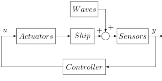
The dynamics of a ship in a seaway, under the linearity assumption, is generally divided into two different parts: first how the ship reacts to its actuators (fins and rudders); second, to the environment, that is to say the wind, waves and current - only waves are considered here. The effects of both are then added, be it expressed in efforts or in movements. It is assumed they can
be computed separately from one another1. The
model is then considered to be the superposition of the motions due to the waves and the motions due to the actuators. So, waves will be taken as a
1
This is not valid from a hydrodynamics point of view. Yet it is a useful and quite correct assumption when applying linear control theory.
disturbance additive on the outputs of the ship’s dynamics, as shown on figure 1.
-u Actuators - Ship - i+ + W aves ? -Sensors y -¾ Controller
Fig. 1. Control model with output additive distur-bance
In addition, it is assumed that the ship has no list, and that no non linear phenomenon appears. The ship’s model is supposed to depend only on speed relative to water.
2.1 Ship dynamics
The ship is fitted with rudders which are used for stabilisation and stabilisation fins; they have different effects on the ship’s motions. The fins are used only for roll stabilisation, and should interfere very little with the heading. On the contrary, rudders have a great influence on roll motions, but are primary used to control the yaw. Yet these effects appear in two quite separated frequency ranges.
The inputs u for the model are the realised ac-tuators position: α for the fins, and δ for the rudders. x is the state of the ship, composed of sway velocity v, roll velocity p, roll angle φ, yaw
velocity r and yaw ψ (x = [v p φ r ψ]T). The
dynamics of the ship on calm sea is modeled by equation 1 and 2. The wave disturbance w only affects the dynamical system output in φ, p, ˙p and ψ. V is the value of the speed of the ship relative to water. The matrices B and C depend on the speed as the roll acceleration is measured.
˙x = A(V )x + B(V )u (1)
y = C(V )x + D(V )u + w (2)
The model is parameterised in speed V . The coefficients of the matrices are dependent on V as second (fins and rudders efficiency, damping), first or zeroth (buoyancy) order polynomials. The measures y considered for control (see equa-tion 3) are the roll angle φ, the roll velocity p, the roll acceleration ˙p and the heading angle ψ.
y = φ + φw p + pw ˙p + ˙pw ψ + ψw (3) 2.2 Actuators
The actuators have a dynamics, that can be modeled by a second order transfer function as in equation 4. α(s) = ω 2 a ω2 a+ 2ζaωas + s2 αd(s) (4)
where αd is the desired, and α is the realised
actuator position.
The parameters ωa and ζa may be determined
by experimental measures. Position and speed of both the rudders and fins are not free. The device itself limits the available position of the fins and rudders. But in addition, as cavitation and mechanical efforts increase with speed, they may become intolerable; the saturation of the fins in position is dependent on speed. Its dependency
is usually realised in 1/V2, see Lloyd (1989). The
other saturation do not necessitate variation of their values.
2.3 disturbance
The disturbance is calculated from the seakeep-ing characteristics of the ship and the sea state spectrum. The sea state spectrum used here is the Bretschneider spectrum (Fossen, 1994):
Sww(ω) = 0.31Hs2 ω4 0 ω5exp µ −1.25ω 4 0 ω4 ¶ (5)
Hs is the significant wave height (mean of the
height of highest third of waves), and ω0 = 2Tπ
0
the dominating wave pulsation.
2.4 Simulation model
The previous sections detail the model used for synthesis. A more realistic model was used to test the control laws. The simulation model still com-prises an output additive disturbance, generated in position (and attitude), speed and acceleration. In addition, it takes into account the temporal non-linear aspects of saturation (in angle and rate for both the fins and rudders) and a comprehen-sive actuators dynamics, and digitalisation of the control law. In addition to this, a pure delay is added in temporal simulations to make up for the information transportation effects in the ship internal network.
3. SYNTHESIS METHODOLOGY 3.1 Review of common synthesis methods
Different control synthesis techniques have been used so far. First methods were based on PID
control with feedback in roll, roll speed and roll acceleration. Other forms of control law also tested are: LQG (Sgobbo and Pearsons, 1999; van Amerongen et al., 1990), neural networks (Liut et al., 2000), pole placement for RRS (Fossen, 1994), sliding mode (Lauvdal and Fossen, 1996). Hearns et al. (2000) proposed a robust controller design through QFT.
The choice of PID coefficients is based on the phase compensation of delays induced by actu-ators servos, and on statistical measures of actua-tors use on a standard sea state (Lloyd, 1989). This give good results as accounted for in the literature. Katebi et al. (2000) exposed a PID tun-ing framework ustun-ing optimisation. They also
pro-posed H∞ control laws which weights are based
on previous works of Grimble et al (1993). In the spirit of Katebi et al. (2000), PID and
H∞ controller are studied. More precisely, here,
a common scheme of optimisation is used to tune controllers of different natures. In the first case this will directly give the PID coefficient. In the
second case this will give the H∞ weights that
are parameterised by a finite (and small) number
of coefficients; the final calculation of the H∞
controller being classical.
The proposed methodology is described in the following paragraphs.
3.2 Principles
The stabilisation problem expressed in common language terms is: ‘use at best the actuators to stabilise the roll, but do not destabilise the yaw nor use too much energy’. In addition to these three requirements, are requirements common in the control field (stability, robustness). This is expressed in the following paragraph.
3.3 Specifications
There are primary two antagonistic objectives: O1 Reduce the roll motion
O2 Use the minimal quantity of energy
The description of the computation is given in the next paragraph. The second objective is necessary to ensure that the two actuators do not compen-sate for one another, case which may appear. This defines a two-goals optimisation problem ; it is tractable conveniently with stochastic algo-rithms such as genetic algoalgo-rithms. It could have been possible to aggregate the different objectives into a unique one typically by linear combination, but consequently loosing the grasp on the optimi-sation meaning. It has then been decided to keep
the different objectives, so as to make the most enlightened choice possible.
The wish not to destabilise the yaw motion while damping roll motions can be understood by a relative use of rudders less than of the fins. This implies a constraint on the relative efficiency of both actuators on the roll reduction. But it has been difficult to obtain solutions with this config-uration of objectives, and another objective was added to express this constraint.
O3 Respect as precisely as possible the reparti-tion constraint
In addition to this, there are constraints that have to be respected, and which correspond to usual stability and robustness constraints, but also to specific requests of the problem:
C1 Controller stability
C2 Closed loop stability under a given control application delay
C3 Acceptable delay margin
C4 Low amplification under and over resonance (two constraints)
C5 Limited saturations for fins and rudders in both position and velocity (four constraints)
3.4 Calculations
3.4.1. Objectives The first objective is expressed
as the minimisation of the roll RMS value on a particular sea state for the closed loop system. The second objective is the sum of the RMS values
of the fins’ and rudders’ positions (resp. σα and
σδ), for the same sea-state.
Objective O3 is evaluated from the RMS values of the actuators positions. The repartition, noted r, is defined (see equation 6) as the weighted ratio ’use of the fins’ over ’total use of the actuators’,
the weights being the H∞ norm of the open loop
transfer functions between fin (Nα) and rudder
(Nδ) position and roll.
r = Nασα
Nασα+ Nδσδ
(6)
3.4.2. Stability constraints The stability of the
controller is tested because of numerical uncer-tainties during the synthesis that may lead it to be unstable.
The closed loop stability is tested through the calculation of the closed loop poles of the system, given a delay in the application of the computed control. The delay is approximated by a Pad´e, and simulates the presence of unmodeled phase, digitalisation and information transfer. The delay margin itself being more precisely evaluated with µ−analysis, as the control problem is MIMO.
3.4.3. Low amplification constraint Constraints C4 are calculated from sensibility transfer be-tween perturbation and output (in roll rotation speed). They require the closed loop not to am-plify roll too much outside the resonance zone (where it dampens the roll).
3.4.4. Actuators saturation constraints - C5 The saturations are impossible to evaluate pre-cisely when working in the frequency domain. It has only a temporal meaning but may be trans-posed to the frequency domain under statistical assumptions.
Under reasonable assumptions2 the expression of
the expected frequency of threshold crossing (at
value α0) in a period of one minute, is:
e+ = 60 2π r m2 m0 exp(−2α 2 0 m0 ) (7) 3.5 Implementation
Multi objective optimisation is conveniently tract-able through a genetic algorithm, though it some-times is slow. They are based on the evolution of ’individuals’ representing potential solutions; at each iteration, the algorithm processes the genes through different operations (selection, mutation, cross-over) to produce a new generation of individ-uals. The algorithm stops when a given number of generations has been achieved.
The outcome of a multi objective problem is not a unique solution, but a set of solution, each being adequate as no supremacy of an objective above another has been set. This set is called the Pareto front. The tricky point is then to choose a particular solution fitted to our problem. The choice is made by the following algorithm. Choose the solution:
(1) that belongs to the Pareto front or is very near
(2) that complies to the repartition constraint (3) that has the best roll reduction
The software used for this work is
modeFRON-TIER3. It is a conception optimisation software,
with a dedicated user interface, several optimisa-tion methods supporting mono or multi-objective designs with constraints.
2
The signals are centered, and have narrow band spectra, and the amplitude repartition of the signals with time respects a Reynolds law (Price and Bishop, 1974; Lloyd, 1989)
3
Developped by ESTECO, see www.esteco.com
4. CONTROL LAWS CALCULATIONS AND SIMULATION RESULTS
The available measures are the roll angle, the roll velocity, the roll acceleration and the heading angle.
4.1 PID
The expression of the control law is :
α =¡K1α+ sK2α+ s2K3α¢ φ
δ =¡K1δ+ sK2δ+ s2K3δ¢ φ +
¡s−1
K4δ+ K5δ+ sK6δ¢ ψ
The coefficients to be optimised are Kiαand Kiδ
for i ∈ {1..3}. The coefficients Kiα for i ∈ {4..6}
are fixed using a simple pole placement method, see (Fossen, 1994). The simulation results are given in tables 1, 2 and 3.
4.2 H∞
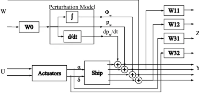
The H∞controller synthesis is based on the
min-imisation of the infinity norm of a given transfer function between weighted input disturbances and weighted controlled outputs. The weights are dy-namical (they have internal states) and are used to shape the closed loop transfer functions. The choice of the weights and the description of the closed loop system is critical for the results. Furthermore, they have to be parameterised for optimisation.
The synthesis principle is given in figure 2. The following paragraph describes the weights.
Fig. 2. H∞standard synthesis model
The different signals disturbing the system are not independent of each other. Only two perturbation
signals are used: pp and ψp, the rest of the
sig-nals being calculated from them by approximated integration and derivation, as shown in the per-turbation model in figure 2.
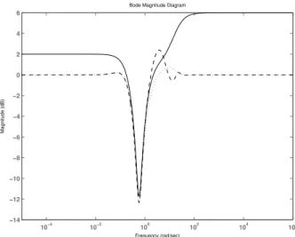
Bode Magnitude Diagram Frequency (rad/sec) Magnitude (dB) 10−4 10−2 100 102 104 106 −14 −12 −10 −8 −6 −4 −2 0 2 4 6
Fig. 3. H∞roll sensibility weight of order 3 (solid),
closed loop sensibility without input delay (dotted) and with input delay (dashed)
4.2.1. Weights The choice of the weights
deter-mine the shape of the sensibility transfer (between disturbance w and the output z). The final aim is to damp the wave induced roll, to keep the actuators efficient and not to saturate them too much (see section 3.3).
The different weights are taken as follows: W0 Filter on the perturbation input, low pass W11 Roll sensibility weight - see section 4.2.2 W12 Yaw sensibility weight;
W12(s) = Krττr1r2s+1s+1, with τr2> τr1
W31 Fin disturbance sensibility weight;
W31(s) = Kfττf 1f 2s+1s+1 with τf 2> τf 1
W32 Rudder disturbance sensibility weight;
W32(s) = Kr
The parameters used for optimisation are Kr, Kf
and the maximal attenuation of roll in the roll sensibility weight. Dynamics in the yaw sensibility weight is meant to compensate in yaw only the low frequency motions; for the fin disturbance sensibility weight, it is meant to avoid using the fins at low frequencies.
4.2.2. Roll sensibility weight This weight
deter-mines the obtained performance. As the best per-formance is to be obtained, it is parameterised so as to be optimised. Different shapes were tested, of different orders. A simple and efficient solution is determining the shape by interpolation from a given number of control points. The figure 3 gives an idea of the shape of this weight for order 3 (solid) and realised closed loops without (dotted) and with (dashed) a delay on the input.
The order of the weight influences the achievable performance as with more parameters it is more easily malleable. But as order of the standard
Table 1. Roll damping performance (%)
Speed P ID H∞1 H∞2
10 56 54 45 15 76 77 63 20 78 82 77 25 72 83 71
Table 2. Fin usage (degrees RMS)
Speed P ID H∞1 H∞2
10 5.81 6.45 8.57 15 4.55 4.97 5.35 20 3.71 4.54 4.95 25 2.08 3.11 3.49
model for H∞ increases the synthesis requires
more time.
4.3 Simulation results
The controllers calculated have been tested on a frigate-like ship (length 120m, displacement 3000 tons). The loading conditions were sea state 5 (Hs=3.25m & T0=9.7s) for an encounter angle of 90. The simulation duration is 20 minutes. The control laws were digitalised and applied at a sampling time of 0.1 second.
The obtained results are given in terms of quality, that is the roll reduction rate of the stabilised ship compared with the unstabilised ship, see table 1. Tables 2 and 3 give the RMS values of the actuators position in degrees.
There is a destabilising effect on yaw control. The RMS yaw signal is increased by 5 to 25% at all
speeds for the H∞controllers, whereas, for PID, it
is increased at lower speeds (10 and 15 knots) and decreased (stabilised) at higher speeds (20 and 25 knots). This behaviour stems from the tuning differences between the controller: the yaw control
bandwidth for the PID is higher than for the H∞
controllers.
The H∞controller with an order 5 roll sensibility
weight (H∞1 in the tables) gives better results
at higher speeds, while the H∞ controller with
an order 3 roll sensibility weight (H∞2 in the
tables) gives equivalent results as the MIMO PID controller. Attention must be paid at the fact that the outcome of the optimisation may be improved, in the three cases: longer optimisation could lead
to equivalent performance between PID and H∞.
Furthermore, the order of the H∞controllers is 18
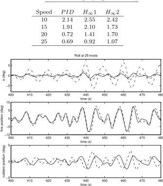
or 20; the complexity induced has to be taken into account as it implies problems of digitalisation and calculations onboard; difficulties finding the appropriate digitalisation method were encoun-tered when applying the controllers in simulation. A typical simulation is given in figure 4 for speed 25 knots.
Table 3. Rudder usage (degrees RMS) Speed P ID H∞1 H∞2 10 2.14 2.55 2.42 15 1.91 2.10 1.73 20 0.72 1.41 1.70 25 0.69 0.92 1.07 400 410 420 430 440 450 460 470 480 −5 0 5 time (s) φ (deg) Roll at 25 knots 400 410 420 430 440 450 460 470 480 −10 −5 0 5 10 time (s)
fins position (deg)
400 410 420 430 440 450 460 470 480 −5
0 5
time (s)
rudders position (deg)
Fig. 4. Simulation for different controllers at speed 25 knots (dash-dotted: unstabilised
ship; solid: H∞1 control; dashed: H∞2
con-trol; dotted: PID control) 5. PERSPECTIVES
The control synthesis problem solved here is not an end in itself. The main purpose of this work is to synthesise gain-scheduled controllers. Usually done with PID, the coefficients are reduced with speed increase, see (Lloyd, 1989). The goal is to
take advantage of the H∞ synthesis method for
its results, and also of the rigourous construction of a gain-scheduled controller via LMIs. Indeed, no theoretical result can prove that the gain-scheduled PID controller stabilises the system. By contrast, gain-scheduled controllers synthesised via LMIs are proven to stabilise the system. Contrary to the common method when controllers are interpolated, it is here the weights that have to be interpolated, and parameterised with the scheduling variables as a polytopic or an LFT model, see (Biannic, 1996; Duc and Hiret, 2001). The controller is then generated from the res-olution of an optimisation problem under LMI constraints.
6. CONCLUSION
In this article is described the methodology used
to tune MIMO PID and H∞controllers for the roll
damping of a ship. The method is multi-objective, and searches the best performance achievable, while respecting stability, robustness and physi-cal constraints. The simulation results show the
interest of H∞ controllers as giving better or
equivalent roll reduction results if finely exploited, though inducing problems of complexity and digi-talisation. Furthermore, the rigourous approaches
to gain-scheduled controllers linked to H∞ give
interesting perspectives.
7. REFERENCES
Biannic, Jean-Marc (1996). Commande robuste
des systmes paramtres variables.
Applica-tions en aronautique. PhD thesis. SUPAERO, Toulouse, France.
Duc, Gilles and Arnaud Hiret (2001). Application au pilotage d’une chane de tangage d’un mis-sile sur un large domaine de vol. APII-JESA (35), 107–125.
Fossen, Thor I. (1994). Navigation and Guidance of Ocean Vehicles. John Wiley & sons. New York.
Grimble, M.J., M.R. Katebi and Y. Zhang (1993).
h∞based ship fin-rudder roll stabilisation
de-sign. In: 10th Ship Control Systems Sympo-sium. Vol. 5. Ottawa, Canada.
Hearns, Gerald, Reza Katebi and Mike Grimble (2000). Robust fin roll stabiliser controller de-sign. In: 5th IFAC Conference on Manoeuver-ing and Control of Marine Crafts. Aalborg, Danmark.
Katebi, M.R., N.A. Hickey and M.J. Grimble (2000). Evaluation of fin roll stabiliser con-troller design. In: 5th IFAC Conference on Manoeuvering and Control of Marine Crafts. Aalborg, Danmark.
Lauvdal, Trygve and Thor I. Fossen (1996). Non-linear non-minimum phase rudder-roll damp-ing system for ships usdamp-ing sliddamp-ing mode con-trol. In: IFAC World Congress, paper is not included in the Proceedings. San Francisco, U.S.A.
Liut, Daniel T., Dean T. Mook, Hugh F. Landand-ingham and Ali H. Nayfeh (2000). Roll reduc-tion in ships by means of active fins controlled by a neural network. Schifftechnik/Ship Tech-nology Research 47, 79–89.
Lloyd, A.R.J.M. (1989). Seakeeping, Ship Be-haviour in Rough Weather. Marine Technol-ogy. Hellis Horwood.
Price, W.G. and R.E.D. Bishop (1974). Probabilis-tic Theory of Ship Dynamics. Chapman and Hall. Londres.
Sgobbo, J.N. and M.G. Pearsons (1999). Rud-der/fin roll stabilization of the uscg wmec 901 class vessel. Marine Technology 36(3), 157– 170.
van Amerongen, J., P.G.M. van der Klugt and H.R. van Nauta Lemke (1990). Rud-der roll stabilisation for ships. Automatica 26(4), 679–690.