T
HE TERM STRUCTURE OF CRUDE OIL FUTURES PRICES
:
A
PRINCIPAL COMPONENT ANALYSIS
Delphine L
AUTIER1Cahier de recherche du C
EREGn° 2004-02
ABSTRACT: This article relies on principal component analysis to identify the movements of the crude oil futures prices’ curve and the contribution of components to volatility. It aims to understand the factors explaining the prices curve’s volatility in order to implement hedging and investment strategies. Applying the principal component analysis to the crude oil futures market leads us to confirm, first of all, previous results reached by others authors in different markets: empirical tests show that three components explain most of the variation of the crude oil prices’ curve. These components are parallel and relative shifts, and curvature. Moreover, we reach two conclusions concerning the evolution of the prices dynamic on a long period of time, and the influence of the futures contract’s maturity on this dynamic. Evidence is given of the permanent nature of the three components, and of the more complex behavior of long-term prices curves.
KEY WORDS: crude oil – futures prices – term structure – principal component analysis. SECTION 1.INTRODUCTION
This article is centered on the movements of the crude oil futures prices’ curve. The term structure of futures prices describes the relationships between the spot price and futures prices for different delivery dates. It is supposed to resume all the information needed to hedge positions on the physical market, to undertake arbitrage operations or to support investment decisions. Thus, understanding the behavior of the prices’ curve is a prerequisite for the use of derivatives instruments. Moreover, permanent factors are required for managing price risk or pricing derivatives.
In the American crude oil market, the concept of term structure is all the more important that there are futures contracts for very far delivery dates: up to seven years. In order to identify the crude oil prices’ movements, to test their stability and to examine whether or not they are independent of the futures contracts’ maturity, we use the method of the principal component analysis, that takes historical data on movements in the prices and attempts to define a set of components or factors that explain these movements.
In the case of interest rates, Litterman and Scheinkman (1991), Knez, Litterman and Scheinkman (1994), and Frye (1997) lead to the identification of three movements characterizing the
prices’ curve. These movements correspond to parallel shifts of the curve (level factor), relative shifts (steepness factor) and deformations (curvature factor). In the case of commodities, Cortazar and Schwartz (1994) show that three factors also explain the dynamic behavior of the term structure of copper prices. Tomalsky and Hindanov (2002) extend the empirical work of these two authors to the petroleum market. They propose a principal component analysis in multicommodity and seasonal markets. Lastly, Borovkova (2003) uses principal component analysis as a way to detect market transitions, form backwardation to contango and back. Our study corroborates these previous works, in the case of the crude oil market. Moreover, we reach two conclusions concerning the evolution of the prices dynamic on a long period of time, and the influence of the maturity on this dynamic. These conclusions constitute the main contributions of this article.
The first conclusion is related to the analysis of the evolution of prices’ behavior on a long period of time. It is the first study on such a long period: thirteen years, from 1989 to 2002. Therefore, it enables the investigation of the eventual structural nature of prices’ movements. Empirical tests show that everything being equal, the same factors (level, steepness and curvature) can be identified on the whole period and that there are little changes in their respective intensity from one period to another. Even an a priori specific period like the first Gulf War does not stand out from the others. Thus, there is a permanent structure of prices’ dynamic.
The second conclusion concerns the influence of maturity on prices’ dynamic. This study includes very far maturities: until seven years for the period 1999-2002. Two principal component analyses are compared on this period: the first relies on futures contracts having a maturity ranging from one to eighteen months, the second takes account of all available maturities, from the first to the
84th month. Empirical tests show that increasing the maturity significantly influences the behavior of
the prices’ curve. Indeed, the first factor looses some of its explicative power, whereas the second and – more marginally – third factors gain in importance. Consequently, even if there are permanent factors in the futures prices’ dynamic, as the crude oil futures market comes to fruition, the introduction of long-term contracts changes slightly this dynamic. This transformation implies that risk management on long-term maturities is more complicated that on short-term ones.
These statements are important for several reasons. Firstly, such a study constitutes a useful prerequisite for the elaboration of term structure models of commodity prices, especially for the crude oil market. Indeed, if two factors are sufficient to explain more than 99% of prices’ volatility, even when the whole curve is taken into account, then it is relevant to retain solely two underlying factors in a term structure model. Secondly, if the steepness factor has a significant impact for long-term maturities, then a long-term analysis should retain a mean-reverting behavior for at least one of the state variables of the model. Thirdly, understanding the prices’ dynamic is important for risk management. Indeed, principal component analysis can be used in order to quantify the risks of a
portfolio, for Value At Risk analysis for example2. Such a tool is all the more interesting that the
dynamic factors are stable.
The remainder of the article is organized as follows. Section 2 presents the method. Section 3 applies it to crude oil futures prices’ curves for different periods and maturities. Section 4 concludes.
SECTION 2.PRINCIPAL COMPONENT ANALYSIS: THE METHOD3
Principal component analysis is a statistical method that reduces the dimensionality of a data set by collapsing the information it contains. In a system including a large number of observed variables, groups of variables often evolve in unison because they are influenced by the same driving forces. Usually, the analysis shows that there are only a few of such driving forces.
The reduction of the dimensionality of the data set is obtained by transforming the initial matrix (n observations × N variables) in a reduced matrix containing M factors and n observations:
= = nM n ij M f f f f f n i M j 1 1 11 ) ,.... 1 ( ns Observatio ) ,.... 1 ( Factors
where fij is the value of the factor j for the observation i and M < N. The problem is simplified by
replacing a group of variables with less new variables.
Principal component analysis gives a tool for achieving this simplification. Indeed, the method generates a new set of variables, called factors or principal components. These principal components summarize the main features of the original variables. They respect two conditions: linearity and orthogonality. The first condition implies that each principal component is a linear combination of the original variables: 1 N j j k
F
a
==
∑
k kf
where F is a factor, X is the original variable, and a is a coefficient.
The second condition signifies that all the principal components are orthogonal to each other:
(
Fj,Fm)
= 0 j≠mρ where ρ is the correlation coefficient.
There are as many principal components as original variables and, taken together, they explain all the variability in the original data. However, the sum of the variances of the first principal components usually exceeds 80% of the total variance of original data. Examining these few first factors authorizes a deeper understand of the driving forces that influence the original data set.
SECTION 3.PRINCIPAL COMPONENT ANALYSIS OF CRUDE OIL PRICES CURVES
The aim of this study is twofold. Firstly, it intends examining the possible structural nature of the crude oil futures prices movements. Secondly, it investigates whether there is an influence of the maturity on this dynamic. Thus, the study examines the prices’ behavior on a long period of time, from June 1989 to January 2002, and it includes long-term futures contracts.
1. Data
The database is an important element of the study. In 2004, the most developed commodity futures market, considering the volume and maturity of the transactions, is the American crude oil
futures market. Working with crude oil futures prices makes it possible to study maturities as far as
seven years4. The data are daily settlement prices for the West Texas Intermediate futures contract
traded at the New York Mercantile Exchange (Nymex). They have been operated such as the first futures price’s maturity corresponds to the one month maturity, such as the second futures price corresponds to the two months maturity, and so forth. As a result of the evolution process of the market, new contracts with longer maturities were introduced during the period. Delivery dates were indeed progressively extended from 15 to 84 months between 1989 and 1999. Consequently, the information relative to long-term contracts is only available on the period 1999-2002.
2. Principal components
The first part of the study aims identifying the dynamic prices’ behavior on the whole period,
from the 06/06/1989 to the 01/14/2002. It includes maturities from the first to the 15th months
(15 × 3163 futures prices). When applying the principal component analysis, there are initially as many original variables as different futures prices of various expiry dates. Thus Table 1, which presents the factors obtained on the whole study period, contains 15 factors.
Table 1. Principal components, 1989-2002.
Factor 1 Factor 2 Factor 3 Factor 4 Factor 5 Factor 6 Factor 7 Factor 8 Factor 9 Factor 10 Factor 11 Factor 12 Factor 13 Factor 14 Factor 15 1 month 0.343 0.5475 -0.6118 -0.4062 0.2022 -0.0432 0.0047 0.0219 -0.007 0.0081 -0.0048 0.003 -0.0003 -0.0004 0.0001 2 months 0.3296 0.378 -0.0206 0.4821 -0.5718 0.3968 -0.0014 -0.1749 0.0236 -0.0055 0.0051 -0.0051 0,0000 0.002 -0.0002 3 months 0.314 0.2352 0.2269 0.3604 0.0499 -0.5919 -0.0128 0.5414 -0.1303 0.035 -0.0209 0.0075 -0.0009 -0.0022 -0.0002 4 months 0.2983 0.1207 0.3197 0.0968 0.379 -0.1825 0.0226 -0.5232 0.4459 -0.2667 0.2233 -0.1005 0.057 -0.0234 -0.0015 5 months 0.2837 0.0325 0.3148 -0.0548 0.2933 0.1679 -0.0084 -0.2356 -0.2942 0.3413 -0.528 0.3161 -0.2437 0.0731 0.0069 6 months 0.2699 -0.038 0.2661 -0.1736 0.1526 0.3258 -0.0472 0.1199 -0.3787 0.1807 0.3109 -0.3807 0.5048 -0.0782 -0.0097 7 months 0.2573 -0.0944 0.1988 -0.2407 -0.0137 0.2924 -0.103 0.3237 0.0209 -0.3019 0.3601 0.0879 -0.6288 0.0373 0.0258 8 months 0.2458 -0.1403 0.1282 -0.2584 -0.1553 0.1373 -0.1383 0.3009 0.4371 -0.268 -0.4405 0.2115 0.4215 -0.0512 -0.0465 9 months 0.2351 -0.1782 0.0533 -0.24 -0.2864 -0.1714 0.853 -0.0789 -0.0787 -0.0301 0.0096 0.0059 -0.0043 -0.0022 -0.0038 10 months 0.2251 -0.2105 -0.0196 -0.1772 -0.2596 -0.1887 -0.2346 -0.0523 0.3101 0.475 -0.0715 -0.4625 -0.1823 0.3429 0.1442 11 months 0.2159 -0.2373 -0.0903 -0.0916 -0.2146 -0.2272 -0.265 -0.1797 -0.0298 0.2515 0.2164 0.2737 -0.0294 -0.6202 -0.3301 12 months 0.2074 -0.2594 -0.1559 0.0123 -0.1112 -0.1799 -0.2246 -0.1962 -0.2949 -0.2007 0.1912 0.383 0.2148 0.3352 0.5125 13 months 0.1993 -0.2777 -0.2137 0.1284 0.0317 -0.0638 -0.1146 -0.1136 -0.288 -0.389 -0.199 -0.2651 -0.0458 0.2765 -0.6059 14 months 0.1918 -0.2932 -0.2637 0.248 0.1851 0.0916 0.0537 0.0412 -0.0298 -0.1587 -0.2717 -0.3403 -0.1435 -0.4989 0.4624 15 months 0.1847 -0.3061 -0.308 0.3606 0.3306 0.2386 0.2189 0.2063 0.2966 0.33 0.2203 0.2662 0.0811 0.2098 -0.1539
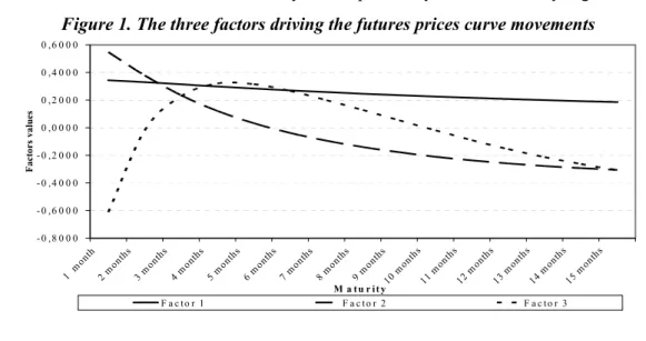
The three first factors are the more easy to interpret. They are illustrated by Figure 1.
Figure 1. The three factors driving the futures prices curve movements
- 0 ,8 0 0 0 - 0 ,6 0 0 0 - 0 ,4 0 0 0 - 0 ,2 0 0 0 0 ,0 0 0 0 0 ,2 0 0 0 0 ,4 0 0 0 0 ,6 0 0 0 1 m onth 2 m onths 3 m onth s 4 m onth s 5 m onths 6 m onth s 7 m onths 8 m onth s 9 m onths 10 m onths 11 m onth s 12 m onths 13 m onths 14 m onths 15 m onths M a t u r i t y Fac tor s val ue s F a c to r 1 F a c t o r 2 F a c to r 3
4However, the transaction volume is not very high for the longer maturities. Therefore, the quality of the information
The first factor corresponds to a roughly parallel shift in the prices curve: all of this factor’s values are positive. Therefore, whatever the maturity considered, one unit of that factor corresponds to an increase of the futures price. The increase is for example around 30 cents for the four months maturity, and 21 cents for the 12 months maturity. The weights decrease with the maturity. Thus, the stronger impact is associated with the nearest futures price. This phenomenon is due to the fact that futures prices have different volatilities. Indeed, one of the most important features of the commodity prices curve’s dynamic is the difference between the price behaviour of first nearby and deferred contracts. The movements in the prices of the prompt contracts are large and erratic, while the prices of long-term contracts are relatively still. This results in a decreasing pattern of volatilities along the prices curve. This phenomenon is usually called “the Samuelson effect”. Intuitively, it happens because a shock affecting the nearby contract price has an impact on succeeding prices that decreases as maturity increases (Samuelson, 1965). As futures contracts reach their expiration date, they react much stronger to information shocks, due to the ultimate convergence of futures prices to spot prices upon maturity. These price disturbances, influencing mostly the short-term part of the curve, are due to the physical market, and to demand and supply shocks.
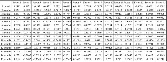
The Samuelson effect can be eliminated by a standardization of the futures prices. In that case, the same role is attributed to each maturity in the definition of the proximity between two observations. Table 1A, in the Appendix, illustrates the results obtained with standardized prices. The most dramatic change concerns the first factor, which appears more clearly as a level factor, because factor’s values are then really close to each other. Whatever the maturity considered, one unit of that factor corresponds to an average increase of around 25 cents of the futures price.
The second factor corresponds to a “steepening” or a “twist” of the prices curve: when the nearest futures prices move in one direction, the deferred prices move in the other one. More precisely, one unit of the second factor corresponds to an increase of the shorter maturities, and simultaneously
to a decrease of the longer maturities. The inflection point is located at the 6th month, and the stronger
impact is associated with the two extremities of the prices curve: it is attributed to the nearest futures
price, which is followed by the 2nd and the 15th months.
The third factor corresponds to a curvature of the term structure. Indeed, futures prices of the
shorter and longer maturities move in the same direction, whereas middle maturities (3rd to 9th months)
move in another one.
These three factors are the most important because they describe virtually all possible futures prices curves. A factor’s importance can be measured by the standard deviation of its factor’s score. Because there are as many maturities as factors in the test presented here, the futures prices changes observed on any given day can always be expressed as a linear sum of the factors, by solving a set of
N simultaneous equations, where N is the number of maturities. The amounts of the factors in the
prices moves, on a particular day, are known as the factor or component scores.
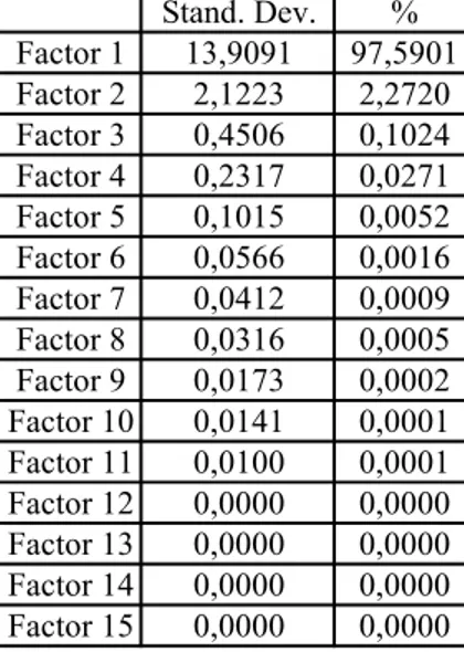
The standard deviations of the factors scores are shown in Table 2. Gathering Tables 1 and 2 shows that a one standard deviation move in the first factor corresponds to the 6 months futures prices
moving by 13.9091×0.2699 =3.75 US dollar, the 15 months futures prices moving by
From the variances of the factors, it is easy to calculate the total variability explained by each principal component. In the case presented here, the total variance of the factors is 198.24. The first factors explains ((13.9091)²/198.24) = 97.59% of this total variance. Thus, the first two factors account for 99.86 % of the variance, the third factor accounts only for 0.10%. Therefore, most of the risk associated with futures prices move is accounted for one or two factors, instead of all 15 futures
prices, and all the other factors can be neglected5.
Table 2. Standard deviation and variability explained by each components, 1989-2002 Stand. Dev. % Factor 1 13,9091 97,5901 Factor 2 2,1223 2,2720 Factor 3 0,4506 0,1024 Factor 4 0,2317 0,0271 Factor 5 0,1015 0,0052 Factor 6 0,0566 0,0016 Factor 7 0,0412 0,0009 Factor 8 0,0316 0,0005 Factor 9 0,0173 0,0002 Factor 10 0,0141 0,0001 Factor 11 0,0100 0,0001 Factor 12 0,0000 0,0000 Factor 13 0,0000 0,0000 Factor 14 0,0000 0,0000 Factor 15 0,0000 0,0000
Some of our results are thus in line with previous studies on interest rates. Indeed, these studies also lead to the identification of the level, the steepening and the curvature factors. What is more specific of commodity prices is that the third factor can actually be neglected, and the second is not really important, as far as these maturities are concerned. Relying on that basis, it is possible to study the eventual structural nature of prices movements, and the impact of the maturity on prices behavior.
3. The permanent nature of principal components
In order to examine the structural nature of prices movements, three different studies are compared. The first corresponds to a long period (1989-2002), the second is centred on a short one (1999-2002), and the third is dedicated to a specific period, during which prices where especially
volatile and backwardation was particularly strong: the 1st Gulf War (1990-1991). The maturities
retained for these studies are similar: respectively 15, 18 and 17 months6.
The examination of the principal components obtained on the two new periods, illustrated by Tables 3 and 4, leads to the identification of the same three factors that were extracted from Table 1.
5 In the case of interest rates, Frye (1997) shows that the first factor accounts for 83.1% of the total variation of the data, the second factor accounts for 10%, and the third factor for 2.8%. In his study, he considers US Treasury rates with maturities between three months and 30 years. Thus, in the case of crude oil futures prices, the importance of the first factor seems to be high. However, with longer maturities (see paragraph 4 of this section), our results are very close to those obtained with interest rates.
6 We retained a 15 months maturity for the period 1989-2002 because it was the farthest maturity for a futures contract in 1989. In 1990-1991, the farthest maturity was 17 months. Lastly, we retained only the 18 first months for the period 1999-2002, in order to make comparisons (see paragraph 4) between short- and long-term futures contracts.
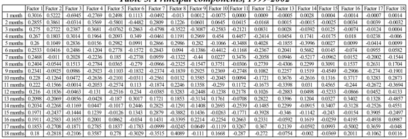
Table 3. Principal components, 1999-2002
Factor 1 Factor 2 Factor 3 Factor 4 Factor 5 Factor 6 Factor 7 Factor 8 Factor 9 Factor 10 Factor 11 Factor 12 Factor 13 Factor 14 Factor 15 Factor 16 Factor 17 Factor 18 1 month 0.3016 0.5222 -0.6945 -0.2769 0.2498 0.1113 -0.0492 -0.013 0.0012 -0.0075 0,0000 0.0009 -0.0005 0.0028 0.0004 -0.0014 -0.0007 0.0014 2 months 0.2855 0.3861 -0.0314 0.3569 -0.5801 -0.4482 0.2809 0.1226 0.0601 0.0645 0.0415 -0.0168 0.0015 -0.0015 -0.0025 0.0034 0.0039 -0.0032 3 months 0.275 0.2722 0.2387 0.3681 -0.0762 0.2863 -0.4798 -0.3522 -0.3087 -0.2583 -0.2121 0.0831 0.0028 -0.0392 0.0125 -0.0074 -0.0124 0.0004 4 months 0.267 0.1803 0.3014 0.1964 0.2093 0.349 -0.0461 0.1191 0.2969 0.454 0.4457 -0.2414 0.0454 0.1741 -0.0175 0.018 0.0238 -0.006 5 months 0.26 0.1049 0.2836 0.0156 0.2982 0.0991 0.2866 0.2986 0.282 -0.1066 -0.3488 0.4028 -0.1855 -0.3996 0.0027 0.0099 -0.0414 0.0099 6 months 0.2533 0.0416 0.2486 -0.1204 0.2778 -0.1572 0.2843 0.094 -0.1386 -0.4412 -0.1168 -0.2367 0.2041 0.5682 0.0145 -0.074 0.0955 0.0582 7 months 0.2468 -0.011 0.2028 -0.2236 0.185 -0.2738 0.0959 -0.1322 -0.44 0.0227 0.3476 -0.2058 0.0946 -0.5217 -0.0962 0.0152 -0.2002 -0.1544 8 months 0.2404 -0.0544 0.1513 -0.2784 0.0365 -0.279 -0.0966 -0.2325 -0.1547 0.3751 -0.0306 0.2739 -0.4306 0.2299 0.3091 0.1537 0.2631 0.1704 9 months 0.2341 -0.0925 0.0986 -0.2923 -0.1103 -0.1832 -0.2374 -0.1839 0.2925 0.2369 -0.2748 0.1082 0.2257 0.1519 -0.4549 -0.2906 -0.274 -0.1901 10 months 0.228 -0.1264 0.0472 -0.2636 -0.2101 -0.0311 -0.2561 0.0132 0.3585 -0.2045 0.0094 -0.1721 0.3676 -0.2616 0.1316 0.3717 0.3283 0.2873 11 months 0.222 -0.1566 -0.0014 -0.2053 -0.2574 0.113 -0.1874 0.2246 0.1358 -0.259 0.1172 -0.1673 -0.3398 0.031 0.4565 -0.244 -0.2672 -0.3694 12 months 0.216 -0.1836 -0.0463 -0.131 -0.2516 0.234 -0.0385 0.3283 -0.2448 -0.1238 0.2178 0.1026 -0.2883 0.0498 -0.5233 -0.0866 0.0452 0.4133 13 months 0.2098 -0.2069 -0.0856 -0.0428 -0.187 0.3017 0.1721 0.1853 -0.3134 0.1761 -0.0708 0.2822 0.3396 0.1204 0.0327 0.3402 0.1328 -0.4857 14 months 0.2034 -0.2268 -0.1169 0.0447 -0.1017 0.2446 0.2825 -0.1291 -0.1408 0.2693 -0.2539 -0.1485 0.2299 -0.0915 0.3407 -0.3128 -0.2526 0.4551 15 months 0.1971 -0.2437 -0.1444 0.1239 -0.0126 0.1343 0.2879 -0.3882 0.1436 -0.0263 -0.1771 -0.3928 -0.346 -0.1142 -0.243 -0.0154 0.3905 -0.2497 16 months 0.1911 -0.2583 -0.1655 0.2001 0.0862 -0.034 0.1431 -0.3395 0.2214 -0.2254 0.2663 0.2331 -0.0592 0.1619 -0.0259 0.4195 -0.4938 0.0987 17 months 0.1853 -0.2708 -0.1871 0.2785 0.1837 -0.1783 -0.0999 -0.0245 0.0649 -0.1119 0.3267 0.367 0.2139 -0.0592 0.0993 -0.5002 0.3659 -0.048 18 months 0.18 -0.2818 -0.2106 0.3587 0.278 -0.3029 -0.3515 0.4089 -0.111 0.1668 -0.287 -0.272 -0.0754 -0.002 -0.0369 0.2011 -0.1062 0.0116
In Table 3 and 4, the parallel shifts (Factor 1) present the same characteristics as those described previously: the weights are all positive, and the more important are attributed to the short
part of the curve. This is especially true for the 1st Gulf War period, where the volatility of the nearest
contracts is particularly high.
Table 4. Principal components, 1990-1991
Factor 1 Factor 2 Factor 3 Factor 4 Factor 5 Factor 6 Factor 7 Factor 8 Factor 9 Factor 10 Factor 11 Factor 12 Factor 13 Factor 14 Factor 15 Factor 16 Factor 17 1 month 0.4128 -0.5231 0.6755 0.3122 0.0261 0.0089 -0.0372 -0.0005 0.0089 -0.0058 -0.002 0.0002 -0.0014 -0.0005 0.0001 -0.0001 0 2 months 0.3838 -0.3438 -0.214 -0.6442 0.4755 -0.2006 0.0854 -0.0032 0.0013 0.0029 0.0023 -0.0088 0.0012 0.0032 0 0.0004 0.0003 3 months 0.3445 -0.1907 -0.2415 -0.2565 -0.6043 0.4891 -0.3411 0.0001 0.0003 0.0046 -0.0006 0.0053 -0.0031 -0.0038 -0.0011 0.0009 0.0014 4 months 0.3097 -0.0566 -0.2728 0.2121 -0.3427 -0.223 0.6659 -0.1926 -0.3235 0.1457 0.0451 -0.0714 -0.0225 0.0009 0.0175 -0.0001 -0.008 5 months 0.2802 0.0307 -0.2696 0.2578 -0.0887 -0.2825 0.0153 0.2069 0.5621 -0.4001 -0.1787 0.3462 0.1408 -0.0252 -0.0483 -0.0054 0.0072 6 months 0.2543 0.0947 -0.2266 0.2756 0.0876 -0.2222 -0.3222 0.3062 0.0828 0.1788 0.2383 -0.5965 -0.2889 0.0727 0.0652 -0.0043 -0.0031 7 months 0.2323 0.1399 -0.1617 0.2391 0.2124 -0.0509 -0.3468 0.0346 -0.3585 0.445 0.0465 0.4719 0.3247 -0.0936 -0.091 -0.0022 0.0047 8 months 0.2131 0.1716 -0.0999 0.176 0.236 0.1381 -0.1689 -0.3205 -0.3419 -0.4081 -0.4721 -0.0334 -0.2609 0.2559 0.1862 0.0499 0.0064 9 months 0.1965 0.1924 -0.0332 0.1069 0.2097 0.2584 0.0309 -0.3988 0.1095 -0.23 0.2493 -0.2536 0.1799 -0.5627 -0.308 -0.0765 0.0101 10 months 0.1822 0.2085 0.0291 0.0395 0.1645 0.3122 0.1681 -0.2267 0.3291 0.1223 0.4244 0.1054 0.1241 0.5626 0.2443 0.0919 -0.0464 11 months 0.1705 0.2225 0.0811 -0.0231 0.1122 0.2771 0.2235 0.1423 0.2357 0.3642 -0.2396 0.2139 -0.5361 -0.3704 0.1923 -0.0321 0.0286 12 months 0.1608 0.2325 0.119 -0.0656 0.0502 0.2021 0.1938 0.2967 0.0079 0.1256 -0.358 -0.2037 0.17 0.3264 -0.6207 -0.1587 -0.0352 13 months 0.1527 0.2411 0.1491 -0.1036 -0.0056 0.0945 0.1313 0.3895 -0.155 -0.1396 -0.0809 -0.1945 0.4292 -0.1831 0.401 0.4589 0.1752 14 months 0.1458 0.2492 0.1722 -0.135 -0.0586 -0.039 0.0293 0.2579 -0.2324 -0.2749 0.2388 0.1054 -0.0079 -0.0434 0.2118 -0.5783 -0.4664 15 months 0.1395 0.256 0.1925 -0.1606 -0.1143 -0.1572 -0.0357 0.0529 -0.1538 -0.1982 0.319 0.2068 -0.2811 0.0851 -0.219 -0.0248 0.6841 16 months 0.1337 0.2621 0.2093 -0.1831 -0.1648 -0.2679 -0.1109 -0.1481 0.0075 0.0013 0.0637 0.0865 -0.2008 -0.0155 -0.2589 0.5714 -0.5072 17 months 0.1283 0.2668 0.2227 -0.2003 -0.2107 -0.3621 -0.1741 -0.401 0.2223 0.2673 -0.295 -0.183 0.2348 -0.0078 0.2294 -0.2913 0.1484
Tables 3 and 4 give also evidence of the presence of a second factor, leading prices to move in different directions according to their maturities. The inflection point is located around respectively
the 7th and 5th months, and the most important weights are once again attributed to the extremities of
the curve. The only difference in the results obtained concerns the signs of the second factor for the 1st
Gulf War period. In that case, the second factor is negative for the nearest maturities, and then positive, whereas it presents the opposite profile on the other periods. Lastly, a third factor can also be
identified. The two inflection points are located around the second and the 10th months, and, one more
time, the period of the 1st Gulf War presents opposite signs.
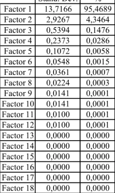
Thus, whatever the period taken into account, three main components can be identified, that characterize the futures prices movements. Moreover, Tables 1, 3 and 4 show that the factors values evolve in the same intervals. This structural nature of prices behavior is even more pronounced if we consider the total variability explained by each component (Tables 5 and 6).
Table 5. Standard deviation and variances of the components, 1999-2002 Stand. Dev. % Factor 1 13,7166 95,4689 Factor 2 2,9267 4,3464 Factor 3 0,5394 0,1476 Factor 4 0,2373 0,0286 Factor 5 0,1072 0,0058 Factor 6 0,0548 0,0015 Factor 7 0,0361 0,0007 Factor 8 0,0224 0,0003 Factor 9 0,0141 0,0001 Factor 10 0,0141 0,0001 Factor 11 0,0100 0,0001 Factor 12 0,0100 0,0001 Factor 13 0,0000 0,0000 Factor 14 0,0000 0,0000 Factor 15 0,0000 0,0000 Factor 16 0,0000 0,0000 Factor 17 0,0000 0,0000 Factor 18 0,0000 0,0000
For all the periods considered, the relative importance of the three factors is similar: the first factor explains at least 95% of the total variance, and gathering the first and second factors account for at least 99.7% of this variance. Thus, it appears clearly that structurally, the first factor has the stronger impact, the second factor a lower one, and that the third factor can be neglected.
Table 6. Standard deviation and variances of the components, 1990-1991 Stand. Dev. % Factor 1 16,4114 97,5787 Factor 2 2,4257 2,1317 Factor 3 0,6920 0,1735 Factor 4 0,5082 0,0936 Factor 5 0,1942 0,0137 Factor 6 0,1241 0,0056 Factor 7 0,0854 0,0026 Factor 8 0,0316 0,0004 Factor 9 0,0173 0,0001 Factor 10 0,0141 0,0001 Factor 11 0,0100 0,0000 Factor 12 0,0100 0,0000 Factor 13 0,0000 0,0000 Factor 14 0,0000 0,0000 Factor 15 0,0000 0,0000 Factor 16 0,0000 0,0000 Factor 17 0,0000 0,0000
This permanent nature of prices movements is important, because it can be exploited for modelling purposes. Our result show, indeed, that only two factors can be taken into account in order to explain the prices behaviour, at least for the shorter maturities (up to 18 months). These two factors are the parallel shift, that stands for upward or downwards movements of the entire curve, and the steepening, that represents changes in the slope of the curve. A mean reverting process can be used in order to characterize this second factor.
Another preoccupation appears however when reaching modelling purposes. Indeed, a model is presumed to be able to represent prices behaviour for every maturity. Until now, however, this study was concentrated on rather short-term delivery dates. Do the results of the principal component analysis change when long-term futures contracts are taken into account? Answering this question constitutes the objective of the next part of this article.
4. The impact of maturity on prices behavior
The analysis of the impact of maturity on prices behaviour is obtained by comparing the
results found on the same period – 1999-2002 – but on different maturities – 1st to 18th months in the
first case, 1st to 84th months in the second case. Tables 7 and 8 present, respectively, the principal
components and their variance for the long-term maturities7.
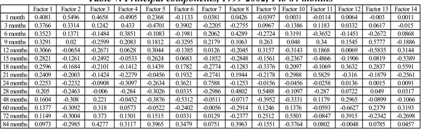
Table 7. Principal components, 1999-2002, 1 to 84 months
Factor 1 Factor 2 Factor 3 Factor 4 Factor 5 Factor 6 Factor 7 Factor 8 Factor 9 Factor 10 Factor 11 Factor 12 Factor 13 Factor 14 1 month 0.4081 0.5496 0.4658 -0.4905 0.2368 -0.1133 0.0381 0.0426 -0.0397 0.0031 -0.0114 0.0064 -0.003 0.0011 3 months 0.3766 0.3314 0.1242 0.433 -0.4701 0.3902 -0.2205 -0.2755 0.0967 -0.1386 0.1183 0.0332 0.0617 -0.015 6 months 0.3523 0.1371 -0.1484 0.3851 -0.1083 -0.1981 0.2062 0.4289 -0.2724 0.3191 -0.3652 -0.1451 -0.2672 0.0868 9 months 0.3291 0.02 -0.2599 0.2083 0.1812 -0.3295 0.2179 0.1063 0.263 0.048 0.34 0.1545 0.5777 -0.1886 12 months 0.3066 -0.0654 -0.2671 0.0628 0.3044 -0.1385 0.0126 -0.2045 0.3157 -0.3143 0.1868 0.0069 -0.5835 0.3144 15 months 0.2821 -0.1261 -0.2492 -0.0533 0.2624 0.0683 -0.1852 -0.2848 -0.1561 -0.2367 -0.4866 -0.1906 0.0819 -0.5389 18 months 0.2596 -0.1684 -0.2101 -0.1412 0.1439 0.1782 -0.2774 -0.1283 -0.3376 0.2097 -0.1069 0.3632 0.2837 0.5591 21 months 0.2409 -0.2003 -0.1424 -0.2279 -0.0456 0.1932 -0.2741 0.1944 -0.2178 0.2988 0.5829 -0.316 -0.1879 -0.2561 24 months 0.2253 -0.2232 -0.0908 -0.3097 -0.2634 0.3621 0.7588 -0.1253 -0.0156 -0.0456 -0.0258 0.0136 0.0015 0.0091 28 months 0.205 -0.2463 -0.006 -0.284 -0.3026 0.0335 -0.2986 0.4802 0.5488 -0.1097 -0.287 0.0722 0.049 0.0317 48 months 0.1604 -0.308 0.221 -0.0452 -0.3876 -0.5312 -0.0511 -0.0717 -0.3952 -0.3331 0.1179 0.2965 -0.0899 -0.1066 60 months 0.1377 -0.3092 0.318 0.0573 -0.0522 -0.2402 -0.0056 -0.2914 0.1246 0.1376 -0.0593 -0.6627 0.2379 0.3193 72 months 0.1149 -0.3004 0.373 0.1501 0.1515 0.0331 0.0129 -0.2377 0.2512 0.5503 -0.0847 0.3915 -0.2342 -0.2698 84 months 0.0973 -0.2985 0.4277 0.3117 0.3965 0.3479 0.0751 0.3963 -0.1551 -0.3764 0.0802 -0.0048 0.0785 0.0457
Table 7 authorizes the identification of the three factors describing the prices movements. The comparison with Table 3 shows that the values of the first factor are less homogeneous when the whole price curve is taken into account. Thus, the shifts of the curve are a less parallel than before, because the differences in the volatilities of the futures prices increase with maturity. As in Table 3, the most important weight is associated to the short-term extremity of the curve. As far as the second factor is concerned, the steepening seems to be a bit more pronounced with longer prices curves. Lastly, the third factor is here totally different: its values are positive for the two ends of the curve, and negative for the intermediate maturities. Table 3 gives evidence of an opposite profile for this factor.
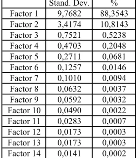
This difference in the third factor is not really important, as Table 8 illustrates it: indeed, the third factor accounts for 0.52% of the total variance of the futures prices… Thus, even if increasing the maturity gives more weight to the curvature factor (with the short-term maturities, its level was 0.15%), this weight is still marginal. What is more important in Table 8 is that the relative importance of the two first factors varies depending on the maturity. Now that the whole prices curve is taken into account, the second factor explains more than 10.8% of total variability, whereas its level was 4.35% with short-term contracts.
7 For this part of the study, 32 different maturities were available, from the 1st to the 28th months, and the 48th, the 60th, the
Table 8. Standard deviation and variances of the components, 1999-2002, 1-84 months Stand. Dev. % Factor 1 9,7682 88,3543 Factor 2 3,4174 10,8143 Factor 3 0,7521 0,5238 Factor 4 0,4703 0,2048 Factor 5 0,2711 0,0681 Factor 6 0,1257 0,0146 Factor 7 0,1010 0,0094 Factor 8 0,0632 0,0037 Factor 9 0,0592 0,0032 Factor 10 0,0490 0,0022 Factor 11 0,0283 0,0007 Factor 12 0,0173 0,0003 Factor 13 0,0173 0,0003 Factor 14 0,0141 0,0002
Comparing the results of principal component analysis on different periods and maturities gives thus key insights about the number and shape of the underlying factors in term structure models of commodity prices. Our results show that for short-term analysis, one-factor models could be retained for prices analysis. However, when the maturity of the contracts increases, it becomes important to integrate a second factor. Lastly, there is no real need of a third factor, because its importance is marginal, even with seven years futures contracts.
SECTION 4.CONCLUSION
Applying a principal component analysis to crude oil futures prices’ curves leads to the identification of the type of prices curves movements. Three different kinds of movements can be distinguished: a parallel shift in the curve (first factor), a steepening of the curve (second factor) and the curvature (third factor). Moreover, the principal component analysis makes it possible to calculate the contribution of each component to volatility. This calculus shows firstly, that when the prices curves are shortened, the importance of the first factor increases dramatically and secondly, that the third factor can always be neglected.
REFERENCES
Borovkova S., 2003. Detecting market transitions: from backwardation to contango and back, EPRM, June, 46-49.
Cortazar G. & Schwartz E.S., 1994. The valuation of commodity contingent claims, Journal of Derivatives, 1(4), 27-39.
Frye J., 1997. Principal of risk: finding VAR through factor-based interest rates scenarios, in VAR:
understanding and applying Value At Risk, Risk Publications, London, 275-288.
Hull J.C., 2003. Options, futures and other derivatives, Prentice Hall, 697 p.
Jackson J.E., 1991. A user’s guide to principal components, John Wiley & Sons, 1-25.
Knez P.J., Litterman R. & Scheinkman J., 1994. Explorations into factors explaining money market returns, Journal of Finance, 49(5), 1861-1882.
Litterman R. & Scheinkman S., 1991. Common factors affecting bond returns, Journal of Fixed Income, 1(1), 54-61.
Samuelson P.A. (1965). Proof that properly anticipated prices fluctuate randomly. Industrial
Management Review, 6, 41-49, Spring.
Tomalsky C. & Hindanov D., 2002. Principal components analysis for correlated curves and seasonal commodities: the case of the petroleum market, Journal of Futures Markets, 22(11), 1019-1035. APPENDIX
Table 1A. Principal components, standardized prices, 1989-2002.
Factor 1 Factor 2 Factor 3 Factor 4 Factor 5 Factor 6 Factor 7 Factor 8 Factor 9 Factor 10 Factor 11 Factor 12 Factor 13 Factor 14 Factor 15 1 month 0.2493 0.5121 -0.592 0.4931 0.2752 0.0691 0.0198 0.0289 -0.0079 0.0123 -0.0056 0.0061 -0.0019 -0.0001 -0.0002 2 months 0.2541 0.4062 -0.1723 -0.3489 -0.5813 -0.4607 -0.1029 -0.2349 0.053 -0.0149 0.0043 -0.0087 0.0035 -0.0022 0.0001 3 months 0.2571 0.3063 0.0817 -0.3906 -0.1302 0.4764 0.1258 0.6058 -0.2159 0.0796 -0.0277 0.0184 -0.0058 0.0005 0.0005 4 months 0.259 0.2166 0.2319 -0.2376 0.2797 0.3286 0.0621 -0.3922 0.4407 -0.3753 0.227 -0.1821 0.0811 0.0746 0.0062 5 months 0.2602 0.1392 0.2866 -0.1023 0.3084 -0.0205 -0.0468 -0.3109 -0.1134 0.3223 -0.4164 0.4363 -0.2967 -0.2387 -0.0221 6 months 0.2608 0.0699 0.2921 0.0399 0.2531 -0.2544 -0.1209 -0.0233 -0.3276 0.3354 0.0914 -0.287 0.5242 0.3317 0.0297 7 months 0.261 0.0082 0.2656 0.1551 0.1207 -0.3141 -0.1641 0.2531 -0.1417 -0.2018 0.3716 -0.2781 -0.5301 -0.2712 -0.0466 8 months 0.2609 -0.0476 0.2214 0.2275 -0.0363 -0.219 -0.1578 0.3533 0.2519 -0.443 -0.2134 0.4761 0.2514 0.1736 0.0678 9 months 0.2606 -0.0988 0.1593 0.266 -0.2201 -0.0757 0.8684 -0.1053 -0.0803 -0.0114 0.0131 0.0005 -0.0055 0,0000 0.0045 10 months 0.2602 -0.1471 0.084 0.2409 -0.2458 0.1505 -0.1698 0.091 0.4485 0.3047 -0.3169 -0.3979 0.1326 -0.3434 -0.1928 11 months 0.2596 -0.1918 -0.0009 0.1802 -0.2505 0.2484 -0.2016 -0.0992 0.1167 0.2945 0.2116 0.111 -0.3533 0.4941 0.4026 12 months 0.2589 -0.2328 -0.0912 0.0818 -0.1756 0.2442 -0.1875 -0.1986 -0.2711 -0.0428 0.3925 0.3314 0.1966 -0.1525 -0.5455 13 months 0.258 -0.2708 -0.1819 -0.0497 -0.0364 0.1365 -0.1145 -0.1653 -0.3717 -0.3172 -0.1952 -0.148 0.1686 -0.3383 0.5679 14 months 0.2571 -0.3067 -0.2695 -0.2017 0.1337 -0.0551 0.0215 -0.0052 -0.109 -0.2112 -0.4112 -0.2443 -0.2601 0.4417 -0.3963 15 months 0.256 -0.3402 -0.3548 -0.3565 0.3072 -0.2547 0.1686 0.2028 0.3285 0.269 0.275 0.1662 0.0955 -0.1698 0.1242