Shock Propagation Across the Futures Term Structure:
Evidence from Crude Oil Prices
Delphine Lautier† Franck Raynaud‡ Michel A. Robe§ March 3, 2018
úWe thank three referees for very helpful comments that have substantially improved the paper. We also thank
Steve Baker, Scott Mixon, Teresa Serra, Casey Petroff, Steve Kane, Andrei Kirilenko, Patrice Poncet, and participants in seminars at the U.S. Department of Energy’s (DOE) Energy Information Administration (EIA), the U.S. Commod-ity Futures Trading Commission (CFTC), the Finance for Energy Markets Research Initiative Lab (FiME, Institut Henri Poincarré, Paris), and the University of Illinois at Urbana-Champaign, and at the 7thInternational Forum on
Financial Risks (IFFR, Institut Louis Bachelier, Paris) and the 2017 AFFI International Conference (Valence, France) for useful suggestions. We thank Gautier Boucher, Pierre-Alain Reigneron, and Jonathan Wallen for research assis-tance. Lautier and Raynaud gratefully acknowledge support from the Finance and Sustainable Development Chair and the FiME Research Initiative. Raynaud also acknowledges the financial support of the Gabriella Giorgi-Cavaglieri Foundation. Robe gratefully acknowledges the financial support received in his capacity as The Clearing Corporation Foundation Professor in Derivatives Trading at the University of Illinois. Robe contributed to this project in a period during which he also consulted for the DOE and the CFTC. No compensation was received from, and no resources were used at, either the DOE or the CFTC for this project. The opinions expressed in this paper are the authors’ only — not those of the DOE, the CFTC, or the U.S. government. Errors and omissions, if any, are the authors’ sole responsibility.
†Université Paris-Dauphine, PSL Research University, CNRS, DRM, Place du Maréchal de Lattre de Tassigny,
75016 Paris, France. Email: [email protected].
‡Department of Computational Biology, University of Lausanne (UNIL), 1001 Lausanne, Vaud, Switzerland, and
Swiss Institute of Bioinformatics (SIB), Lausanne, Switzerland. Email: [email protected]
Shock Propagation Across the Futures Term Structure:
Evidence from Crude Oil Prices
Abstract
To what extent are futures prices interconnected across the maturity curve? Where in the term structure do price shocks originate, and which maturities do they reach? We propose a new approach, based on information theory, to study these cross-maturity linkages and the extent to which connectedness is impacted by market events. We introduce the concepts of backward and forward information flows, and propose a novel type of directed graph, to investigate the propagation of price shocks across the WTI term structure. Using daily data, we show that the mutual information shared by contracts with different maturities increases substantially starting in 2004, falls back sharply in 2011-2014, and recovers thereafter. Our findings point to a puzzling re-segmentation by maturity of the WTI market in 2012-2014. We document that, on average, short-dated futures emit more information than do backdated contracts. Importantly, however, we also show that significant amounts of information flow backwards along the maturity curve – almost always from intermediate maturities, but at times even from far-dated contracts. These backward flows are especially strong and far-reaching amid the 2007-2008 oil price boom/bust.
Keywords: Mutual information, Market integration, Information entropy, Shock
propaga-tion, Directed graphs, Term structure, Futures, Crude oil, WTI.
1 Introduction
Commodity futures markets fulfill the key economic functions of allowing for hedging and price discovery. In these markets, two important questions arise.
First, are futures prices interconnected across the maturity curve? In theory, they should be linked through the cost-of-carry relationship. In practice, such market integration requires cross-maturity arbitrage. Büyük ahin, Harris, Overdahl, and Robe (2009), however, document that even the three largest U.S. commodity futures markets did not witness substantial trading activity in longer-dated derivatives until 2003-2004 (crude oil) or later (corn and natural gas). This empirical fact suggests the possibility of changes in cross-maturity linkages in the past fifteen years.
Second, assuming that different-maturity futures prices are interconnected, where in the term structure do price shocks originate — and which other parts of the term structure do they reach? Is the direction of the shocks’ propagation stable over time? A conventional view takes the physical market as the place where the absolute price emerges as a function of the supply and demand for the underlying asset. In turn, the derivative market allows for relative pricing: futures prices derive from the spot price. Price shocks should thus spread from the underlying asset to the derivative instrument. Yet, amid a massive increase in far-dated commodity futures trading after 2003, might one not expect to also observe price shocks propagating from the far end to the short (physical) end of the futures curve?
There is, to our knowledge, no theoretical model studying these questions in a setting where multiple maturities of futures contracts trade simultaneously. In this paper, we investigate market integration and shock propagation empirically through the prism of the theory of information. We introduce the concepts of “forward” and “backward information flows” across the term structure, and we rely on net transfer entropies to construct a novel type of directed graph linking all the parts of the term structure. Our laboratory is the New York Mercantile Exchange’s (NYMEX) market for West Texas Intermediate (WTI) light sweet crude oil futures. This market provides an ideal setting for our analysis: among all commodity markets in 2000-2017, WTI futures boast the highest level of trading activity together with the greatest number of far-out delivery dates.
The theory of information, first outlined in a seminal paper by Shannon (1948), studies the measure, storage, and quantification of information. A key concept, in this theory, is “entropy” —
the amount of uncertainty associated to a random variable. In our paper, the information entropy H(R·) of the price return R on a crude oil futures contract of maturity · is a quantity that captures
the degree of uncertainty associated to R·. In other words, H(R·) measures how much we don’t
know about that oil futures’ price return.
In this setting, we use the concept of “mutual information” to investigate futures market integra-tion across maturities. When two variables are interdependent (as is the case, for example, for two times series of futures price returns with two different maturities), the mutual information measure gives the amount of entropy that is reduced (i.e., the amount of uncertainty that is resolved) com-pared to the case where the two variables are independent (Shannon and Weaver, 1949; Schreiber, 2000). Computing the mutual information between contracts is thus analogous to assessing their integration or return co-movements. In contrast to other methods such as Pearson correlations, this probabilistic approach does not require making any assumption about the functional form of the relationship between the variables under consideration.
We find substantial variations over time in the amount of mutual information shared by crude oil futures with different delivery dates. In general, intermediate-maturity contracts (six months to two years) share relatively more mutual information than other contracts do. For all contracts, cross-maturity mutual information increases dramatically after 2003 (amid tight oil supply conditions, a dramatic growth in backdated crude oil futures trading, and the onset of commodity markets’ financialization) and reaches a peak at the top of the oil price boom in summer 2008. It falls back sharply in 2012 (to pre-2005 levels), and drops further in 2013 and 2014 (to pre-2002 levels). It has since recovered dramatically. Taken together, these term-structure findings point to a puzzling re-segmentation by maturity of the WTI market in 2012-2014.
We also investigate the propagation of price shocks across the futures term structure, relying for this purpose on the concept of “transfer entropy” (Schreiber, 2000) that allows for dynamic analyses and for the determination of directionality. It enables us to answer the following question: does a shock to the price return of a futures contract with maturity · at time t beget a shock at time t+ 1 to a futures contract with another maturity? Determining directions is important, as it allows us to ascertain whether price shocks evolve from short-term to long-term maturities or vice versa. Focusing on directionality relates our work to extant studies of Granger (1969) causality — but in a non-parametric world. The technique can also be compared to the exploration of volatility spillovers
(as in Adams and Glück (2015) or Jaeck and Lautier (2016)) while allowing for non-linearities — a crucial advantage given ample evidence that the dynamics of cross-market contagion (i.e., shock propagation) are non-linear.1
On average across our 2000-2017 sample period, we find that contracts with maturities up to 21 months emit more information entropy than do more backdated contracts — a pattern consistent with the traditional view of how futures market function. A dynamic analysis, however, reveals that the amount of entropy emitted by other parts of the curve is non-trivial and can be high at times. Moreover, the directions of the entropy transfers (from near-dated to far-dated contracts or vice-versa) is not stable over time. In particular, an analysis of information entropy flows that run “forward” (i.e., from near-dated to further-out maturities) vs. “backward” (i.e., from backdated to nearer-dated contracts) shows that the backward flows are actually higher than their forward counterparts in 2008, i.e., during a 12-month period encompassing the peak of the 2007-2008 oil price boom and the subsequent price collapse after the Lehman crisis.
Finally, we utilize those non-parametric measures to define a metric that allows us to build an original type of directed graphs. The latter complement our other tests and provide a powerful visualization tool — as well as a means to detect anomalies — for our high-dimensional data. Indeed, insofar as all the futures prices that we study create a system, the latter is complex: it comprises many components that may interact in various ways through time. To wit, on any day in our sample, after discarding illiquid maturities, there remain 33 different WTI futures delivery dates: hence, we have 528 pairs of maturities to examine after accounting for directionality. Moreover, such linkages may change through time as a result of evolving market conditions or trading practices. Finally, chances are few that the relationships between different maturities are always linear.
A graph gives a representation of pairwise relationships within a collection of discrete entities. Each point of the graph constitutes a node (or vertex). In our analysis, a node corresponds to the time series of price returns on a futures contract for a given maturity over a specified period of time. The links (“edges”) of the graph can then be used in order to describe the relationships between nodes. More precisely, the graph can be weighted in order to take into account the intensities and/or the directions of the connections. We do both on the basis of information theory.
There are several ways to enrich the links of a graph. In the finance literature on commodity
markets, for example, the connections between the nodes have been tied to the correlations of returns (e.g., Lautier and Raynaud, 2012), variance decompositions of return volatilities (Diebold, Liu, and Yilmaz, 2017), or the activities of futures market participants (e.g., Adamic, Brunetti, Harris, and Kirilenko, 2017). Here, we rely on the theory of information in order to determine the intensities of the links and obtain their direction. To our knowledge, such an application is original in both the finance and commodity literatures.
The use of graph theory in this context allows us to examine precisely where the information entropy is transferred in the futures price system, and how far throughout the term structure it flows in practice. To that effect, we construct a reference graph that depicts the average behavior of the system in 2000-2017. In part, we find that this benchmark graph supports a conventional view of how a futures market operates — specifically, the notion that price shocks are thought to form in the physical market (here represented by the short maturities) and transmit to the paper market (here made up of further-out maturities). At the same time, however, we find that intermediate maturities send out substantial amounts of information entropy not only to further-dated contracts but also to near-dated ones. Furthermore, a dynamic analysis shows that there are sometimes major changes in the organization of the cross-maturities connections. The biggest such rearrangement is in Fall 2008, with the direction of information flows “flipping” entirely (i.e., originating at the far end of the curve and reaching even the shortest maturities). To the best of our knowledge, while this kind of reverse information-flow patterns is theoretically conceivable, our analysis provides the first empirical evidence of their existence.
Section 2 summarizes our contribution to the literature. Section 3 outlines our methodology, which is based on mutual information and transfer entropy. Section 4 presents the data. Section 5
summarizes our entropy findings. Section 6 is devoted to directed graphs. Section7 concludes.
2 Literature
We contribute to three literatures: on term structures and cross-maturities market segmentation, on causality, and on the use of graph theory in the context of financial and commodity markets.
Questions related to the impact of market imperfections on cross-maturities segmentation — defined as a situation in which different parts of the price term structure are disconnected from each
other — date back to the works of Culbertson (1957) and Modigliani and Sutch (1966) regarding “preferred (maturity) habitats” in bond markets. Spurred by interest rate behaviors observed dur-ing the 2008-2011 financial crisis and the so-called Great Recession, the past ten years have seen a resurgence of theoretical and empirical work documenting increased bond market segmentation dur-ing periods of elevated market stress.2 In commodity markets, research on possible cross-maturity
segmentation across the futures term structure has to date remained purely empirical.3 It deals
almost exclusively with the crude oil market, which boasts high trading volumes and (in the United States) contract maturities extending up to seven years. In contrast to interest rate markets, extant papers find evidence of market segmentation prior to 2003 but conclude that the 2008-2011 financial crisis did not bring about a re-segmentation across maturities in the crude oil space.4
Our paper adds to this prior work in several ways — by quantifying the mutual information shared by contracts of different maturities, assessing the direction of the information entropy flows between maturities, and documenting how these measures evolve over time. Our analyses, while based on different techniques, are consistent with prior findings of increasing crude oil market integration through 2010. However, unlike the cross-maturity integration that characterized the 2004-2011 period, we document that different parts of the WTI term structure became much less integrated in 2011 and, especially, in 2012-2014. Furthermore, we show that, when discussing market segmentation, one must distinguish between transfers of information entropy that flow “forward” vs. “backward” across the term structure — because both types of flows are not always equally impacted by segmentation. In particular, we discover situations (most notably in 2007-2008) when
2For example, D’Amico and King (2013) document the 2009 emergence of a “local supply” effect in the U.S. yield
curve amid the Federal Reserve’s unprecedented program to purchase $300bn worth of Treasury securities. Gürkaynak and Wright (2012), who review this literature, conclude that “the preferred habitat approach (has) value, especially at times of unusual financial market turmoil” (p. 360).
3Theoretical work on the term structure of futures prices for commodities in general, and crude oil in particular,
includes many distinguished contributions such as Schwartz (1997), Routledge, Seppi, and Spatt (2000), Casassus and Collin-Dufresne (2005), Casassus, Collin-Dufresne, and Routledge (2007), Carlson, Khokher, and Titman (2007), Kogan, Livdan, and Yaron (2009), Liu and Tang (2010), and Baker (2016). The models proposed in those papers, however, do not deal with the possibility that market frictions (e.g., limits to arbitrage or informational asymmetries) may prevent different parts of the futures price curve from moving in sync. A different part of the literature on com-modity price formation analyzes the role of spot markets in revealing trader information. That body of work comprises theoretical work by Stein (1987) and Smith, Thompson, and Lee (2015), as well as empirical work by Ederington, Fernando, Holland, and Lee (2012) on crude oil. Those papers highlight the role of physical inventories. Instead, we investigate empirically how and how much information travels across the term structure of a large commodity futures market.
4Based on the informational value of futures prices, Lautier (2005) finds cross-maturity segmentation during the
1990’s but argues that this market segmentation weakens after 2002. Using recursive cointegration techniques and term structure data from 1995-2011, Büyük ahin et al. (2011) find cointegrated WTI futures prices in 2003-2011.
backward flows are actually (and atypically) higher than their forward counterparts.
Finally, the present paper belongs to a growing literature that uses graph theory to investigate price connections across space and/or across markets for equities (e.g., Wang, 2010; Dimpfl and Peter, 2014) and commodities (e.g., Haigh and Bessler, 2004; Haigh, Nomikos, and Bessler, 2004; Lautier and Raynaud, 2012; Diebold, Liu, and Yilmaz, 2017). Compared with this body of work, our article innovates along two main dimensions.
First, at the technical level, we utilize another type of graph based on the theory of information. Building on mutual information and entropy transfers, our graph-based analyses allow us to study all the cross-maturity connections in the WTI futures market, within a non-parametric setting. Our methodological choice allows us also to deal with possible non-linearities and with the sheer size of the system we consider (528 daily pairs of futures maturities after accounting for directionality).
Second, while the spatial dimension of market integration has been analyzed in depth elsewhere for equities and currencies as well as for commodities, the time dimension has not. Most papers investigate the relationship between spot and futures prices5 and simply abstract from term
struc-ture issues. A few papers do look at price integration across maturities (Lautier and Raynaud, 2012; Büyük ahin et al., 2011), but no prior study investigates the information entropy emitted (or received) by commodity futures of different maturities or the direction of the resulting information flows across a commodity term structure. Our paper does. We document for the first time that, while on average more information entropy flows forward than backwards, the backward flows are far from trivial, the intermediate maturities play an important informational role (sending entropy forward and backward), and the information entropy flows across the WTI term structure change not only in magnitude and but also in direction during the “great oil price boom/bust” of 2007-2008.
3 Methodology
This Section presents several concepts for two series of futures price returns corresponding to a pair of contract maturities, which Section 5 will generalize in order to study the interdependence and
5In that context, a key empirical question is whether price discovery takes place on the futures or the spot market
(Garbade and Silber, 1983). While early studies tend to rely on Granger causality to provide an answer, a number of papers apply other techniques in an attempt to tease out causality when the relationship between prices might be non-linear — see, e.g., Silvapulle and Moosa (1999), Switzer and El-Khoury (2007), Alzahrani, Masih and Al-Titi (2014) and references cited in those papers. Kawamoto and Hamori (2011) do look at WTI futures contracts with maturities up to nine months, but their focus is on market efficiency and unbiasedness – not on information flows.
directionality of price movements for multiple futures contracts. Throughout the paper, we rely on the theory of information based on the notions of entropy proposed by Shannon (1948). Section
3.1 presents the concept of “mutual information” (Shannon and Weaver, 1949) that quantifies the dependency between two random variables — which we use as a proxy for market integration. Unlike correlations, the mutual information measure captures non-linear relationships between variables; however, it does not allow for studying the propagation of information. For that purpose, Section
3.2 introduces Schreiber’s (2000) transfer entropy measure.
3.1 Mutual information
In what follows, we consider a time series of price returns for a given futures maturity · as a discrete random variable R· with an empirical probability distribution p(R·). We start from the
interdependence of a pair of futures contracts. This measure of their interdependence, also called “mutual information,” relies on the use of several quantities: the “information entropy” of one variable, as well as the conditional and joint entropies of two variables. These different measures are linked to each other.
A first step is to consider the “information entropy” H(R·) of the futures price return for a
given maturity ·. This quantity captures the degree of uncertainty associated to the variable R·.
In other words, it measures how much we don’t know about that price return. H(R·) is maximum
when all the possible realizations of R· are equally likely.
Formally, following Shannon (1948), we define the information entropy H(R·) associated to the
futures prices’ returns for a given maturity · as: H(R·) = ≠
ÿ
r
p(r·) log p(r·) (1)
where qr is the sum over all the possible values of R· and log denotes the base 2 logarithm. Note
that this quantity increases with the number of possible values for the random variable; for a binary random variable, its value ranges between 0 and 1 — a fact that we shall exploit for the empirical analysis in Section 5.
Next, consider the case of two maturities ·1 and ·2, and the interdependency between R·1 and
unknown of R·1 if the values of R·2 are known is captured by the notion of “conditional entropy,”
i.e., the entropy of R·1 conditionally on R·2:
H(R·1|R·2) = ≠ ÿ r·1,r·2 p(r·1, r·2) log p(r·2) p(r·1, r·2) (2) Using the conditional probability distribution of the two variables p(r·1|r·2), equation (2) becomes:
H(R·1|R·2) = ≠
ÿ
r·1,r·2
p(r·1, r·2) log p(r·1|r·2) (3)
Another interesting quantity is the “joint information entropy” H(R·1, R·2). It quantifies the
amount of information revealed by evaluating R·1 and R·2 simultaneously. This symmetric measure
is related to the conditional entropy described by equations (2) and (3) as follows:
H(R·1, R·2) = H(R·1|R·2) + H(R·2) = H(R·2|R·1) + H(R·1) = H(R·2, R·1) (4)
On the basis of these definitions, it is now possible to define the “mutual information” M(R·2, R·1).
This quantity measures the amount of information obtained about one variable through the other. The mutual information M(R·2, R·1) gives the amount of uncertainty that is reduced when two
variables are interdependent, compared to the case where the two variables are independent: M(R·1, R·2) = H(R·1, R·2) ≠ H(R·1|R·2) ≠ H(R·2|R·1) = M(R·2, R·1) (5)
The mutual information is thus a symmetric quantity. Equations (1), (2), and (5) together yield: M(R·1, R·2) = ÿ r·1,r·2 p(r·1, r·2) log p(r·1, r·2) p(r·1)p(r·2) (6) In this article, we use the mutual information as a measure of the integration of the crude oil futures market in the maturity dimension. This quantity indeed includes what would have been obtained with synchronous correlations between pairs of futures prices’ returns, due to the common history of the returns, and/or to common shocks. Compared with correlations however, this probabilistic approach does not rely on any assumption regarding the behavior of futures returns.
3.2 Transfer entropy
To analyze the propagation of shocks along the futures term structure, we need to account for time lags and directions. We aim to answer the question: does a shock to the return of a given maturity ·2 at time t ≠ 1 induce a shock at time t to another maturity ·1? Directions allow us to assess
whether price shocks evolve from short-dated to long-dated contracts, or vice-versa. This idea is closely linked to Granger causality, but in a non-parametric world. It is also related to volatility spillovers, except for the fact that it allows for non-linear interdependencies between variables.
Starting from the information entropy, a natural way to proceed is to rely on the notion of “transfer entropy” motivated and derived by Schreiber (2000). This measure quantifies how much information entropy (or uncertainty) is transported between dates t ≠ 1 and t from one variable to another (in our case, from one futures maturity to another). It relies on transition probabilities rather than on static probabilities.
Relying on the definition of conditional entropy described by equation (3), and introducing time into the analysis, allows for defining a new quantity: the “entropy rate” h. Two kinds of rates can be distinguished, according to the type of dependence under consideration. First, the entropy rate ht(R·1) quantifies the uncertainty on the next value of R·1 if only the previous state of R·1 matters:
ht(R·1) = ≠
ÿ
p(rt
·1, r·t≠11 , r·t≠12 ) log p(rt·1|rt·≠11 ) (7)
Second, the entropy rate ht(R·1|R·2) quantifies the uncertainty on the next value of R·1 if the
previous states of R·1 and R·2 both have an influence:
ht(R·1|R·2) = ≠
ÿ
p(rt
·1, rt·≠11 , rt·≠12 ) log p(r·t1|rt·≠11 , rt·≠12 ) (8)
With these dynamic measures defined, it is possible to introduce directions into the analysis. The “transfer entropy” T from R·2 to R·1 is the difference between the two rates:
Tt,R·2æR·1 = ht(R·1) ≠ ht(R·1|R·2) = ÿ p(rt·1, r·t≠11 , rt·≠12 ) logp(r t ·1|rt·≠11 , r·t≠12 ) p(rt ·1|r t≠1 ·1 ) (9) This transfer entropy measure is equivalent to Granger causality in the case of a linear
depen-dency between two Gaussian random variables — see Barnett, Barrett, and Seth (2009). Compared to Granger causality, however, transfer entropy presents the major advantages of being model-free and of holding in the case of non-linearity.
Equipped with the above definitions, we can provide an insightful analysis of the propagation of price shocks along the term structure, for all maturity pairs and all directions. As needed, in Section5 we extend these pairwise concepts to the case of multiple maturities. Then, in Section6, we utilize these concepts in the framework of graph theory.
4 Data
We obtain, from Datastream, the daily settlement prices for all NYMEX WTI light sweet crude oil futures contracts between January 2000 and January 2017. We roll futures based on prompt-contract expiration dates and construct 33 time series of futures prices. The first 28 are for the 28 nearest-dated contract maturities (i.e., contracts with 1 to 28 months until expiration). The other five time series correspond, respectively, to contract maturities of 30, 36, 48, 60, and 72 months.
Our empirical analyses use daily returns, computed as: r· = (ln F·(t) ≠ ln F·(t ≠ t)) / t,
where F·(t) is the price of the futures contract with maturity · on day t and t is the time interval,
measured in calendar days, between consecutive sample days (i.e., between business days).
Figure 1 depicts the evolution of WTI futures prices and price returns in our sample period. For readability, we focus on the nearby, one-year out, and two-year out futures. The right-hand side panel of Figure 1 shows that return volatility is lower for the two longer-dated contracts than for the nearby contract, an empirical reality consistent with the Samuelson (1965) hypothesis that price volatility should increase as a futures contract’s maturity nears.6
Obvious in the left-hand side panel of Figure 1 are the oil price boom of 2004-2008 (peaking in mid-July 2008) and the consequent bust in Fall 2008. Equally notable, and especially relevant to the present study, are the differences between the price paths of nearby vs. longer-dated contracts prior to 2004 and again in 2012-2014. We know from prior research (Lautier, 2005; Büyük ahin et al., 2011) that the one-year (two-year) futures prices did not move in sync with the nearby price prior to 2003 (2004) but started doing so soon thereafter. Figure 1 confirms and extends those prior
6We obtain the same volatility ranking when we use the preponderance of the open interest (rather than calendar
findings by showing that: i) starting in late 2012, a “disconnect” reappears between short-dated and further-dated WTI futures; ii) this disconnect, however, disappears after 2014.
5 Empirical Results: Entropy Measures
Section5.1 presents empirical evidence on the mutual information shared by crude oil futures with different maturities and on the evolution of this mutual information over time. Section 5.2 then introduces directionality and examines information entropy flows across the term structure of prices. Section 5.3relates some of our findings to the Samuelson (1965) effect.
5.1 Mutual Information: A Proxy for Market Integration
Changes in the WTI futures market during the period under consideration can be characterized through the lens of mutual information. Recall from Section 3.1 that the mutual information measure quantifies how much we know about the return R·1 given that the return R·2 is known. In
other words, this quantity captures the synchronous moves in prices. In what follows, we distinguish between the mutual information shared by all the futures contracts under consideration vs. the mutual information attached to one specific maturity.
5.1.1 Mutual information shared by all maturities
On the basis of equation (6), which defines the mutual information Mt(R·1, R·2) for a pair of WTI
futures maturities ·1 and ·2, we define the average mutual information shared at date t by all N
futures prices’ returns, MN
t , as follows:
MtN =< Mt(R·i, R·j) >i,j>i (10)
where: a) N is the total number of maturities each day in the sample; b) the Mt(R·i, R·j) are
the elements of the (N ◊ N) matrix of mutual information computed on day t using daily returns for the prior year;7 c) <>
i,j>i denotes the averaging operator over the relevant contract maturities
7To obtain mutual information measures, we need to compute the joint and conditional entropies in equation (5).
We proceed as follows. For any futures price return R·, we retain two possible states: either a positive or a negative
value. In the case of a positive value, the number +1 is affected to the observation; otherwise ≠1 is retained. We then empirically determine the probabilities p(1) and p(≠1) associated to each maturity on a specific window of time. As
(i = 1, 2, ..., N; i < j Æ N).
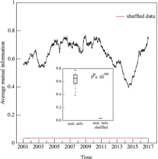
Figure 2 depicts the dynamic behavior of MN
t in 2000-2017 and establishes the statistical
sig-nificance of our results. To assess sigsig-nificance, we start by generating a counterfactual dataset by “shuffling” (using permutations of) the time index of the original dataset (Marschinski and Kantz, 2002). The resulting “shuffled” time series of futures returns have the same mean and variance as the original ones, but temporal relationships are removed. Next, we compute the mutual informa-tion associated to the shuffled data. Figure2shows that, in contrast to the mutual information MN t
associated with the original price series (plotted in black), the counterfactual mutual information (plotted in red, based on the shuffled series) is always close to 0 and does not display any systematic pattern over time. Finally, we establish that the actual and shuffled mutual information series are statistically significantly different using a Welch’s t-test. It is an adaptation of the Student’s t-test that is more reliable when the two samples under consideration do not have the same variance. The associated p-values, denoted by pW in Figure2, give the probability that the null hypothesis cannot
be rejected. As these probabilities are very low, the results can be considered as significant. Figure2 establishes two important empirical facts. First, the mutual information shared by all maturities starts to rise sharply in 2004 and takes very high values from mid-2004 through most of 2010: MN
t generally fluctuates between 0.7 and 0.75, vs. a theoretical maximum of 1 (see footnote 7).
These high values are evidence of synchronization in the prices changes across maturities.8 Insofar
as an increase in MN
t can be interpreted in terms of greater integration of the futures market for
crude oil during that period, this first result complements and extends to many more maturities a key finding of Büyük ahin et al. (2011), based on 1983-2010 data, that the nearby, one-year out, and two-year out WTI futures prices are statistically significantly cointegrated starting in mid-2004.
Second, Figure2 shows that MN
t starts to decrease sharply after December 2010, before falling
we are interested in pairs of futures prices returns, for any pair there are four possible states: (1, 1), (1, ≠1), (≠1, 1) and (≠1, ≠1). When computing entropies, we therefore need a window that is long enough to have sufficiently many observations for each state. We set the window length at a year or 250 trading days (the results are qualitatively similar if we use 2-year rolling windows). Note finally that, as each element of the mutual information matrix analyzes a pair of variables and as we compute the conditional values on the basis of two states (a positive and a negative one), the highest possible value for the mutual information is 1: the results are normalized by the base 2 logarithm.
8In this sense, the mutual information can be compared with the co-movements captured by a Principal Component
Analysis (PCA). More precisely, an analysis of the returns of commodity prices shows that the first factor extracted through the PCA represents parallel moves in the term structure. It can thus be associated to the co-movement in prices (see, e.g., Cortazar and Schwartz, 1994). In our 2000-2017 dataset, the first factor of the PCA explains more than 95% of the variability of WTI futures returns and displays a very high correlation (+0.69) with our measure of mutual information. These results are available from the authors upon request.
even more precipitously in 2013-2014 (reaching its 2000-2017 minimum of 0.39 in June 2014). This finding is novel. It provides formal support for our interpretation of the price patterns depicted by Figure 1 and discussed in Section 4: in 2013 and 2014, different parts of the term structure of WTI futures prices became (temporarily) much less integrated.
A natural question is what explains this temporary re-segmentation of the WTI market across futures delivery dates. Büyük ahin et al. (2011) attribute the WTI futures market’s cross-maturity integration in 2004-2010 in large part to huge increases in far-dated futures trading and in calendar-spread trading by hedge funds and other financial institutions, amid what has been dubbed the “financialization of commodities” (Cheng and Xiong, 2014). On the one hand, as those authors’ dataset ends in mid-2010, their trading-related findings might seem irrelevant to the behavior of the mutual information after 2010. On the other hand, financialization did not end in 2010: pub-lic data from the U.S. Commodity Futures Trading Commission (CFTC) on weekly WTI futures trader positions show that both the WTI non-commercial open interest and calendar spread trading continued to increase from 2010 through 2014 — suggesting that a different explanation, unrelated to the levels of futures trading, may9 have to be found for the evolution of MN
t in 2011-2014.
Interestingly, the decrease of MN
t seen in Figure2starts at the very end of 2010 and comes to a
halt in late 2014. Those four years coincide almost exactly with a period of historically exceptional levels of the Brent-WTI price spread amid a partial geographic segmentation of the world’s crude oil markets – events that Büyük ahin et al. (2013) link to a temporary divergence between crude supply-side conditions in North America vs. in the rest of the world.10 Our findings thus point to the
need for further research in order to assess the extent to which those physical market developments had implication beyond commodity price spreads and into the amount of mutual information shared across the WTI term structure.
5.1.2 Mutual information for each contract maturity
Figure3gives more insight into the term structure developments detected in Figure2, by depicting the mutual information for each individual contract maturity over the course of our sample period.
9Ruling out trading-related explanations would require disaggregated CFTC data, which are not publicly available. 10Fattouh (2010), Pirrong (2010), and Büyük ahin et al. (2013) also analyze a less severe episode of Brent-WTI
price dislocation in 2008-2009 that was due largely to infrastructure constraints at the delivery point for WTI futures in Cushing, OK. Those infrastructure issues had been mostly (completely) resolved by 2011 (2013-2014).
Precisely, for each futures maturity ·i and each day of the sample period t, Figure3 plots the level
of mutual information that this maturity shares with all other maturities: Mt(R·i) =< Mt(R·i, R·j) >j,j”=i
This level is temperature/color-coded in Figure3, ranging from cold/blue (low mutual information) to green, yellow, orange, and hot/red (high mutual information).
In general, Figure3shows that not all futures prices have the same levels of mutual information. Strikingly, at any given time in our sample period, there is much more mutual information at the intermediate maturities (defined as contracts expiring in 6 to 27 months): contracts at both extremities of the futures maturity curve share less mutual information with other contracts than the intermediate-maturity ones do. Furthermore, except for the last five months of 2008 and in 2012-2014, the graph temperature is typically cooler at the very short end of the term structure (plotted at the top of the graph) than at the far end of the curve (at the bottom of the same graph), indicating that the nearest-dated contracts usually contain the least mutual information. This finding is consistent with the notion that short-dated crude oil futures prices are more volatile — sending more information and thus sharing less mutual information.11 Overall, these results
suggest that the WTI futures term structure consists of three main segments: from the 1st to the 3rd months, from the 4th to the 27th months, and finally the most distant delivery dates (contracts maturing in 30 months and beyond).
Figure3also documents that, as a rule across the universe of maturities, the mutual information i) is much higher in 2004-2011 than in 2001-2003 and, especially, than in 2012-2014, and ii) returns to this very high level after 2015. The middle part of the maturity curve, where the amount of mutual information is the highest, is also fatter in 2004-2011 than in the three years before or after. In other words, Figure 3establishes that the market integration phenomenon observed in Figure 2
comes principally from what happens at intermediate maturities.12
11See Robe and Wallen (2016) for recent evidence on the term structure of WTI implied volatilities.
12Figure4complements Figures2(mutual information over time, across all maturities) and3(mutual information
over time for each individual maturity) by depicting the information that a specific maturity shares on average with all other maturities in 2000-2017. It shows that the average mutual information is a hump-shaped function of contract maturity, with a maximum near the 18-month maturity. It also confirms that the intermediate maturities (6 to 27 months) share substantially more mutual information than contracts both at the back end of the curve (shown up to 6 years out) and at the front end – especially the nearby contract.
Finally, we know from Figure2that an important market development took place in 2011-2014, with the total mutual information MN
t falling after December 2010 and reaching record low levels
in 2014. Figure 3 shows that, while the graph temperatures drop across the entire spectrum of maturities during that period, they cool off the most in the case of backdated contracts (those with maturities greater than three years).
5.2 Transfer Entropy between Maturities
This Section investigates cross-maturity linkages through the lens of the entropy transfers between contract maturities. It adds to the insights already gained from the mutual information analyses in Section 5.1by answering the question of which part of the term structure is the shock transmitter and which one is the receiver. We first perform a static analysis across the whole sample period (Section 5.2.1), and then carry out dynamic analyses in order to assess how the typical emission and reception patterns evolve over time (Section5.2.2). Finally, we define and compute “backward” and “forward information flows” across the term structure (Section5.2.3).
5.2.1 Static analysis: Sample-average transfer entropies associated to each maturity We start by computing the transfer entropies over the entire sample period. This approach gives us a picture of the “average” behavior of the system, i.e., it shows whether one maturity sends on average more than what it receives or vice-versa. Starting from equation (9), which focuses on the transfers between two maturities ·1 and ·2, we extend this pairwise measure and compute — for
every trading day t in our sample — the total amount of entropy sent from the futures prices’ return with maturity ·i to all other maturities ·j (j ”= i):
Tt,RS
·i =
ÿ
j”=i
Tt,R·iæR·j (11)
Similarly, we define the daily quantity received by maturity i from all the other maturities as: Tt,RR
·i =
ÿ
j”=i
Tt,R·iΩR·j (12)
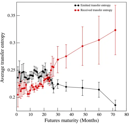
over all trading days in our sample period. The black line in the figure shows the total amount of information entropy emitted by each maturity, using 2000-2017 averages of the daily values computed using Equation (11). The red line shows the total amount of information entropy received by each contract, based on Equation (12). The vertical bars in the figure represent, for each maturity, the average sample variance recorded for the specific measure; these variances are particularly large for the entropy received by the long-dated contracts.
Figure 5 shows that, on average, maturities up to two years (including the 24-month contract) emit more than they receive. For contract maturities beyond 24 months, the average information entropy emitted by a contract is decreasing in its maturity — with an especially sharp drop at 60 months. The average information entropy received exhibits the opposite pattern: it is lowest for the first 24 maturities, and highest for maturities of 25+ months (with the maximum value reached at the back end of the term structure). Intuitively, these static results imply that crude oil market participants whose “preferred habitat” (Modigliani and Sutch, 1966) is the back end of the maturity curve are, on average, more likely to be the object of a shock than to be the source of one.
5.2.2 Dynamic analysis: Transfer entropies over time, by maturity
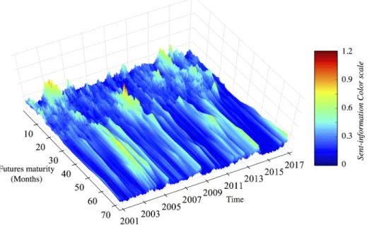
For each maturity ·i and every trading day t in 2000-2017, Figure 6 plots the total entropy Tt,RS ·i
sent from ·i to all the other maturities. Figure7 plots Tt,RR·i, the total entropy received by ·i from
all the other maturities.
Together, these three-dimensional plots show that the short (1-3 months) and/or intermediate maturities (6-27 months) send out the most information entropy (see Figure 6) while the longer maturities (30+ months) are those that receive the entropy (see Figure 7). As such, for much of 2000-2017, the daily entropy transfer patterns match the average (“static”) pattern of Section5.2.1. Figures 6 and7, however, also show that those typical patterns are turned on their head between mid-2007 and early Fall 2008. Very large transfer entropies start being sent by futures with matu-rities from 12 to 27 months (it is the only time when those matumatu-rities are yellow or red in Figure 6). At the same time, not only the long-dated contracts (as is typical) but also the nearest-dated futures (which is atypical) become the recipients of exceptionally large transfer entropies (see Figure
7). For the three nearest-dated contracts, the differences between the entropies received and sent are much larger (especially between July 2007 and July 2008) than at all other times in 2000-2017:
in essence, the nearby, first- and second-deferred contracts turn almost silent for much of that year. As shown in Figure 1, this episode coincides with the oil price “boom/bust of 2007-2008” (Sin-gleton, 2014). It is truly exceptional: at no other time in the sample period do the nearest-dated contracts receive so much information entropy nor do the intermediate maturities send out as much entropy. As such, the 2007-2008 period deserves more attention: we therefore explore it further, using directed graphs, in Sections 6.3and 6.4.
5.2.3 Forward and Backward Information Flows The transfer measure TS
R·i [resp. TRR·i] defined by equation Equation (11) [resp. Equation (12)]
captures the total entropy sent [resp. received] by a single maturity, no matter the direction of this emission [resp. the origin of this reception]. However, if we want to gain insights into the direction in which price shocks propagate, then we need to restrict the analysis to what is emitted in a single direction only, from any maturity.
To this end, we propose the notions of “forward” and “backward” information flows. We define the daily “forward flow” of information, „F, as the sum across maturities of the transfers of entropy
from each maturity ·i to all further-out maturities ·j:
„Ft = N ÿ i=1 ÿ j>i Tt,R·iæR·j (13)
whereqj>i denotes summations over all the maturities greater than i. The “backward flow” „B is
defined analogously as:
„Bt = N ÿ i=1 ÿ j<i Tt,R·iæR·j (14)
On any given day, the forward (backward) flow captures the propagation of price shocks in the direction of longer-dated (shorter-dated) futures.
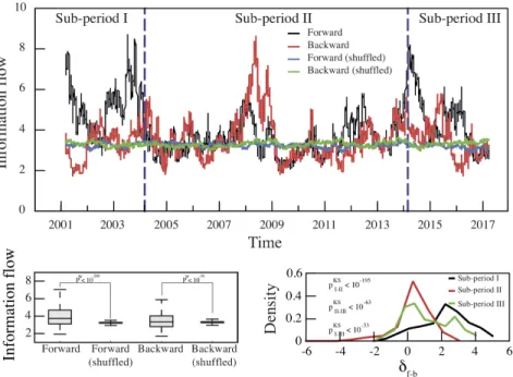
The top panel of Figure8plots the forward and backward flows (graphed, respectively, in black and in red) computed, using a rolling 1-year window, for each trading day from January 2001 to January 2017. The bottom-left panel of the same figure is devoted to significance tests on those information flows. Relying on the methodology developed for the mutual information, it shows that the flows associated to real data are statistically significantly different from those associated with
counterfactual data where the time index has been randomly shuffled.13
Figure8’s top panel distinguishes three main sub-periods in our sample. In almost all of 2000-2003 and much of 2014-2017 (“Sub-periods I and III” in Figure 8), the forward flows are higher than the backward flows: in economic terms, the term structure of WTI futures prices is generally more prone to influence from shocks arising at the near-end of the maturity curve. From 2004 through the Winter of 2014 (“Sub-period II”), in contrast, the amplitudes of the two information flows are generally similar: in other words, the driving forces of price movements are broadly equal all along the term structure, with price shocks propagating in the backward direction as easily as in the backward direction. Figure8even highlights a year in Sub-period II (2008) when the backward flows are not only exceptionally high but are, in fact, much stronger than the contemporaneous forward flows. This period, which includes the peak of the oil price boom (in the first half of 2008) and the subsequent crude price collapse (in the late Summer and Fall of 2008), is the same outlier that we already detected — using other information measures — in Sections 5.1.1and 5.2.2.
A natural question is whether the relative strengths of forward vs. backward flows are statis-tically significantly different across sub-periods. The bottom-right panel in Figure 8 answers in the affirmative by analyzing the difference between forward and backward flows, ”f≠b. The panel
depicts the densities of distribution of ”f≠b in each sub-period. Sub-period I, shown in black, is
clearly characterized by higher forward flows. This is also the case for sub-period III (in green), which exhibits a bi-modal distribution. Sub-period II (in red), in contrast, is centered around null values. The same panel also provides the results of Kolmogorov-Smirnov (KS) tests. The notations pKS
I≠II correspond to the p-values of a KS test comparing the distribution of ”f≠b in sub-period I
with that of ”f≠b in sub-period II. The probability that these two distributions are the same is
extremely low. The same conclusion obtains for pKS
II≠III and pKSI≠III. 5.3 Discussion: Links with the Samuelson Effect
Our findings on forward and backward information flows raise questions regarding the so-called Samuelson effect. Samuelson (1965) hypothesizes that futures price volatility increases as the
con-13We generate counterfactual forward- and backward-flow measures by “shuffling” the time index of each dataset.
The resulting forward information flows are shown in blue (“Forward shuffled” in the figure) and the backward flows are in green (“Backward shuffled”). Unlike the actual forward and backward flows (depicted in black and red, respectively), the counterfactual information flows fluctuate little. Crucially, their values are almost equal for all t.
tract approaches expiration. Some theoretical models explain that effect.14 Other models, though,
predict that futures price volatility may instead decrease as expiration nears.15
Extant theoretical papers’ results on the Samuelson effect have direct implications for the relative volatility of futures with different maturities. Taken as a whole, they show that it is possible for the futures price volatility to be either increasing or decreasing across the term structure. Insofar as price volatility is related to the arrival of information, it might be tempting to conclude that the same models also predict that information could flow either forward or backward across the futures curve depending on circumstances – a possibility that Figure8 establishes as an empirical fact.
In those models, however, a single futures contract trades at any point in time, and this contract moves closer to maturity each period — ruling out the possibility that information could flow in both directions across the term structure. We are not aware of any theoretical model that predicts a key informational role for intermediate maturities (Section 5.2.2), or why backward flows would dominate on 37 percent of all trading days in 2000-2017 (Section 5.2.3). In fact there is, to our knowledge, no model studying how market participants reveal information during price formation in a setting where multiple maturities of futures contracts trade simultaneously. Our empirical findings point to the need for such theoretical research.
Our results show that, in practice, there are price shocks coming from the far end of the crude oil futures term structure that spread to shorter maturities, and vice-versa. An important question is how far they travel — in particular, are shocks at the far end of the futures curve strong enough to spread to the nearby contract and, thus, to the physical market? Section6answers this question.
6 Directed graphs
In this Section, we bring the non-parametric transfer entropy measures of Section 5.2.1 into the framework of graph theory, which is ideal for large-scale analyses. This innovation allows us to carry out an analysis of price shock transmission for all maturity pairs (528 daily links in our case). We propose a directed graph that shows not only the directions of the pairwise transfer entropies,
14Bessembinder et al.(1996), for example, identify conditions under which the Samuelson effect holds — such as
asset markets in which spot price changes include a temporary component (so that investors expect mean-reversion). Note that a number of reduced-form term structure models generate a Samuelson effect without modeling it.
15Anderson and Danthine (1983), for instance, show that “volatility may increase or decrease as delivery approaches
depending upon the pattern of information flow into the market (ibid., p. 257). Hong (2000) shows that the volatility-maturity relationship changes depending on whether market participants are symmetrically informed.
but also their strength, based on the net amount of entropy transported between two maturities (Section6.1). We then use data from the entire sample to compute a benchmark graph representative of the average functioning of the market (Section6.2). Next, we develop a measure of the “distance” between this sample-average graph and the graphs that we compute, using a one-year rolling window, for every day in 2000-2017. We find that, while the information flows across the term structure do generally follow the patterns seen in the benchmark graph, there are exceptions. From Fall 2004 to Fall 2005, and again from Fall 2007 to Winter 2009 (a period that includes the 2007-2008 oil price boom/bust, Lehman Brothers’ bankruptcy, and physical infrastructure issues affecting WTI futures), the cross-maturity information flows differ substantially from the benchmark case (Section
6.3). Finally, we conclude with a case study of the differences between the graph computed for the most “pathological” day in 2008-2009 (October 8, 2008) and the benchmark graph (Section 6.4).
6.1 Building Graphs using Transfer Entropy
A graph is defined by its nodes and links (or “edges”). We assign to each node the time series of price returns for a specific futures maturity. In our case, a graph thus has N = 33 nodes.
In order to enrich the links of the graph regarding the direction and the intensity of the net transfer entropy between each given pair of nodes ·i (i = 1, ..., N) and ·j (j ”= i), we define a daily
“directionality index” Dt,R·iR·j as follows:
Dt,R·iR·j =
Tt,R·iæR·j ≠ Tt,R·jæR·i
Tt,R·iæR·j + Tt,R·jæR·i (15)
The value of the index Dt,R·iR·j, which is bounded by ≠1 and 1, expresses the strength of the link
between the maturities ·i and ·j.16 Its sign gives the direction of the net entropy transfer: from R·i
to R·j when Dt,R·iR·j >0, and from R·j to R·i otherwise.
6.2 The Benchmark: The Sample-Average Directed Graph
To create a benchmark directed graph for the WTI futures market, we compute sample-average directionality indices. Based on equation (9), we start by using one-year rolling windows to compute
16We define the normalized quantity D
t,R·iR·j to capture the strength of the directionality, rather than the quantity
of information transmitted (on which Section5.2focuses instead). A variant of Equation (15), using its denominator’s maximum across contracts, would capture the latter quantity.
the transfer entropies Tt,R·iæR·j, from each contract maturity ·i to each other maturity ·j, for every
trading day. Next, we average those daily values across our 2000-2017 sample. Finally, we input those N(N ≠ 1) = 1, 056 averages into equation (15). This process yields 528 average directionality indices, which we denote ¯DR·iR·j (i = 1, ..., N; j ”= i).
6.2.1 Capturing the graph’s rich content
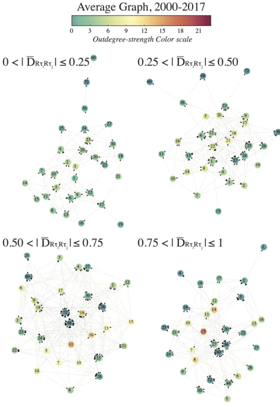
The resulting benchmark graph, with its dozens of nodes and hundreds of links, is very difficult to read. To make its interpretation easier, we filter it according to the strength of the connections between its nodes. Figure 9 depicts four filtered benchmark graphs, ranked in order of increasing link intensity ¯D. For example, the top-left panel focuses on the benchmark graph’s weakest links: | ¯DR·iR·j| < 0.25; the top-right panel only shows links with 0.25 Æ | ¯DR·iR·j| < 0.5; etc.
In addition to the intensity of the graph’s links, it is useful to also keep track of the number of indegrees (outdegrees) at each of its nodes — that is, the number of nodes from which (to which) a given node receives (sends) net transfer entropy. A node’s number of indegrees in Figure9is readily seen by counting, across the four panels, the arrows reaching that node. In order to simultaneously depict the average number of outdegrees from each node while preserving readability, we color-code the nodes from blue (few outdegrees) to green, yellow, orange, and red (many). At each node, across the four panels, indegrees and outdegrees together sum up to N ≠ 1 = 32.
6.2.2 Findings
The most obvious stylized fact in Figure9is that the links between maturity pairs are concentrated in the bottom two panels: put differently, on a typical day in 2000-2017, the information-related strength of most cross-maturity linkages is high. Figure 9also shows where, on average, the infor-mation entropy flows from and where it flows to.
We already know from Figures 5 to7that far-dated WTI futures typically send little information but receive information from the rest of the term structure. Figure9refines this finding by showing that, in net terms, long-dated futures receive a lot of entropy from many different other maturities (lots of arrows hit nodes 30 through 72, and the vast majority of those arrows are seen in the bottom two panels where | ¯D| Ø 0.5) and, conversely, are net senders of entropy to very few other maturities (these same nodes’s colors are blue or teal in all four panels). Figure 9 tells us more than Figures
5 to 7, by showing that some of the information reaching the longest maturities comes all the way from the nearest-dated contracts. To wit, the bottom-left (top-right) panel shows high (moderate) net transfer entropies from the nearby, first-deferred, and second-deferred contracts to all futures maturities between 30 and 72 months (24 to 29 months). In that sense, the benchmark directed graph appears to support a conventional view of how a futures market operates — specifically that price shocks are thought to form in the physical market (here represented by the short maturities) and transmit to the paper market (here made up of contracts with maturities of two years or more). We also know from Figures 5 to7, though, that many middle maturities (5 to 21 months) emit more entropy than they receive. Figure9goes beyond that finding by showing that those substantial net transfer entropies from middle maturities flow not only to further-out maturities but also to the shorter-dated futures. As a matter of fact, the biggest recipient of entropy from the middle of the term structure is the front-month contract (top-right panel). This finding calls for new theoretical work that would generate such a role for the intermediate maturities in a commodity futures market.
6.3 Dynamic Analysis: Daily Distance from the Benchmark Case
The directionality index also allows for dynamic analyses. On the basis of one-year rolling windows, we compute, at each date t, the instantaneous directionality matrix Dt,R·iR·j. This lets us construct
daily directed graphs, whose properties and evolution over time we can examine. A important point of interest regarding the properties of daily directed graphs is their stability: do the directions in the graph evolve during the period? If so, then how?
To answer these questions, we start from the benchmark case (the sample-average directed graph built on the basis of the matrix of directionality ¯DR·iR·j) and measure the distance between that
benchmark graph and the daily directed graphs. Our distance metric is the “survival ratio” or the proportion of links that retain the same direction in both graphs (Onnela, 2003). Here, we compute the daily average survival ratio SRt between the benchmark and daily graphs as:
SRt= 2 N(N ≠ 1) N ÿ i=1 ÿ j”=i ID t,R·i R·jfl ¯DR·i R·j (16)
where the averaging is across maturities, and ID
t,R·i R·jfl ¯DR·i R·j is an indicator function that takes
stability of the graph’s directionality: it tallies up the edges with the same directions in both graphs, and expresses that sum as a proportion of the total number of elements in each graph, N(N≠1)2 . If SRt= 1, then the two graphs are identical in the sense that all the edges in both graphs have the
same directions. At the other extreme, if SRt= 0, then the set of directed links is totally different.
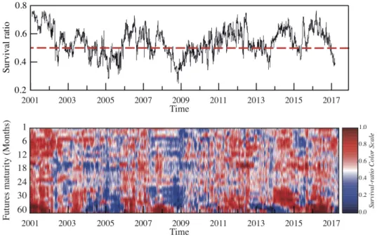
The top panel of Figure 10 shows the distance between the benchmark graph and each of the daily graphs, measured through the time series of the survival ratios SRt. The daily survival ratio
fluctuates between a maximum of 76% and a minimum of 24%; two thirds of the time, it is higher than 50%. This pattern indicates that in our sample period, day after day, a majority of the directed links are in the same state as in the benchmark case. The panel, however, also highlights two periods when the information flows change massively. The first such episode starts in late Fall 2004 and ends approximately a year later. The second episode, during which SRt reaches its lowest sample
value, starts in mid-2008 and ends in Spring 2009.
In order to connect these two episodes with physical and futures market developments, we use the bottom panel of Figure 10. It reveals the maturities most affected by any reorganization of the graph. On a given day t, each maturity ·i is color-coded based on its survival ratio that day
(ranging from dark blue for the lowest values, to dark red for the highest values). Precisely, we compute and plot SRt,·i (i = 1, ..., N):
SRt,·i = 1 N≠ 1 N ÿ j”=i ID t,R·i R·jfl ¯DR·i R·j (17)
During the first episode (2004–2005), Figure10’s bottom panel pinpoints the far-out maturities as contributing the most to the graph’s reorganization — i.e., to the change in the pattern of shock propagation. It complements Figure 6 which shows that, during that period, futures of 2+ years send out uncharacteristically large amounts of information (for the first time ever). Interestingly, this very period witnessed a profound change in WTI trading activity, with open interest in WTI futures with maturities of 3+ years quadrupling compared to 2003 levels amid the financialization of commodity markets (Büyük ahin et al., 2011). Thus, our findings point to the need for a theoretical model in order to assess the extent to which financialization could bring about such changes in cross-maturity informational linkages.
maturities contribute to the graph reorganization, so do the near-dated contracts – but only in the Fall of 2008 and Winter of 2009. Interestingly, that period starts with the demise of Lehman Brothers and continues with a massive steepening of the WTI futures curve amid a petroleum storage-capacity crisis at the WTI futures delivery point in Cushing, Oklahoma — see Büyük ahin et al. (2013). Once again, the methodology we have proposed is able to capture the impact of these market developments on information flows across the term structure.
6.4 A Case Study: October 8, 2008
Figure 10’s top panel shows that the survival ratio SRt hits its two lowest values for the
2000-2017 period in Fall 2008. The first (26%) is reached on September 18 — three days after Lehman Brothers’ bankruptcy, two days after AIG’s takeover by the U.S. Federal Reserve, and one day after the rescue of HBOS (the UK’s then largest mortgage lender) by Lloyds. The other (24%) is reached three weeks later, on October 8, “amid the worst ever week for the Dow Jones.”17
Figure11 provides the filtered graphs for a case study of the information flows across the WTI term structure on October 8, 2008. It is organized and color-coded exactly like Figure 9, allowing for easy comparisons with the sample-average directed graph. As such, several stylized facts emerge. First, in Figure 11, most of the links are in the top left panel — where |DOct8,R·iR·j| Æ 0.25
(Section 6.2.2). In Figure 9, in contrast, | ¯Dt,R·iR·j| Ø 0.5 for most links.18 In plain English, not
only is the direction of the net information entropy transfer different from its sample-average for more than three quarters of the 528 maturity pairs (SROct.8 = 0.24), but the strength of most of
the pairwise directionality indices is also lower on October 8, 2008 than during much of 2000-2017. Second, we know from Figure 5 that, on average, far-dated futures (30+ months) send little en-tropy to other maturities while receiving substantial amounts of enen-tropy from those other maturities (Section 5.2.1). Furthermore, we know from Figure 9that far-dated futures are net entropy recipi-ents from virtually all the other maturities — including from the nearest-dated contracts (Section
6.2.2). We also know from Figures 6 and7, however, that these patterns are turned on their head in 2008 — with the front months becoming the recipients of very large transfer entropies (Section
5.2.2). What Figure11tells us — but the other figures could not reveal — is that, three weeks after
17The Guardian (https://www.theguardian.com/business/2012/aug/07/credit-crunch-boom-bust-timeline). 18Figure12provides a histogram of the link strength in Figures9and11.
Lehman’s collapse and amid a massive crude oil price plunge, the pattern is completely reversed: • In the average graph, the only nodes that send net entropy to many other nodes (color coded
yellow or orange) correspond to maturities between 8 and 19 months. On October 8th, in contrast, the warmest maturities correspond to maturities of 21+ months. Indeed, almost all of the nodes for futures of 21+ months are color-coded yellow, orange, or even red.
• On October 8th, all the far-dated contracts are net senders of entropy to most other maturities, including the nearest-dated ones. To wit, the 6-year futures (node 72) hits the nearby with a medium-strength net transfer (top-right panel of Figure 11), and it hits the first-deferred with a high net transfer (bottom-left panel of Figure 11).
The graph computed for October 8, 2008 is based on a one-year rolling-window of returns. Hence, the fact that the lowest value of SRt is reached on October 8, 2008 implies that the entire
prior year — corresponding to the oil price boom/bust of 2007-2008 — is characterized by highly unusual information flows across the term structure. The extant literature on the financialization of commodities focuses on the impact of index traders and hedge funds’ trading activities on spot or nearby-futures prices, including the possibility that they may cause bubbles — see, e.g., Singleton (2014) and Sockin and Xiong (2015). Our case study’s findings suggest that other components of the futures curve, as well as the informational relationships between them, may be impacted too.
7 Conclusion
We apply the notions of mutual information and transfer entropy to investigate empirically the nature of pricing relationships across the WTI crude oil futures term structure in 2000-2017. In this setting, information refers to the uncertainty associated to a variable. It captures unexpected changes, typically a shock in the futures prices’ return.
We use the level of mutual information across maturities as a proxy for market integration, and we introduce the notions of forward (backward) information entropy flows as proxies for the extent to which price shocks propagate in the direction of longer-term (shorter) maturities. Our forward and backward flows are conceptually related to volatility spillovers, but allow for non-linear interdependencies between variables and for the analysis of a high-dimensional system (here, a term