Synergy Modelling and Financial Valuation : the contribution of Fuzzy Integrals

Synergy Modelling and Financial Valuation : the

contribution of Fuzzy Integrals

Xavier BRY

(CEREMADE, Université de Paris Dauphine)

Jean-François CASTA

(CEREG, Université de Paris Dauphine)

ABSTRACT :

Financial valuation methods use additive aggregation operators. But a patrimony should be regarded as an organized set, and additivity makes it impossible for these aggregation operators to formalize such phenomena as synergy or mutual inhibition between the patrimony’s components.

This paper considers the application of fuzzy measure and fuzzy integrals (Sugeno, Grabisch, Choquet) to financial valuation. More specifically, we show how integration with respect to a non additive measure can be used to handle positive or negative synergy in value construction.

Keywords : Fuzzy measure, fuzzy integral, aggregation operator, synergy, financial valuation. INTRODUCTION

Financial assessments are characterised by: the importance of the role assigned to human judgement in decision making, the use of qualitative information and the dominant role of subjective evaluation. The aim of the article is to examine the specific problems raised by the modelling of synergy between the assets of a firm. As a process which aggregates information and subjective opinions, the financial evaluation of the company raises very many problems relating to issues such as measurement, imprecision and uncertainty. The methods used in the process of financial evaluation are classically based on additivity. By construction, these methods abandon the idea of expressing phenomena of synergy (or redundancy, nay mutual inhibition) linked to over-additivity (or under-additivity) that may be observed between the elements of an organised set such as a firm's assets. This synergy (respectively redundancy) effect may lead to a value of the set of assets greater (resp. lower) than the sum of the values of all assets. This is particularly the case in the presence of intangible assets as good will. We will explore the possibilities offered by non-additive aggregation operators (Choquet, 1953; Grabisch et al., 1995; Sugeno, 1977) with the aim of modelling this effect through fuzzy integrals (Casta and Bry, 1998; Casta and Lesage, 2001).

1. FINANCIAL ASSESSMENTS AND ACCOUNTING MODEL

The strictly numerical approach which underlies the accounting representation is not easily compatible with the imprecise and/or uncertain nature of the data or with the ambiguity of concepts such as imprecision and subjectivity of the accounting valuations, poorly defined accounting categories, subjective nature of any risk evaluation method (see: March, 1987; Zebda, 1991; Casta, 1994; Bry and Casta, 1985; de Korvin et al., 1995; Casta and Lesage, 2001).

Moreover, because its computation structure stems from elementary arithmetics, the traditional accounting model is not designed to handle features linked to synergy.

For these problematic issues, we propose extensions of this model which deal with the synergy affecting the data used in the elaboration of financial statements. However, this approach requires a thorough re-examination of the semantics of the accounting measurement of value and income of the firm.

Our discussion concerns the operating rules governing quantification used in accounting. These rules are based on a rigorous conception of "numericity" which relates back to a given state of mathematical technology linked to the concept of measurement used.

1.1. Measure Theory and Accounting

Generally speaking, Measure Theory, in the mathematical sense, relates to the problem of mapping the structure of a space corresponding to observed elements onto a space allowing numerical representation; the set R of real numbers for example. The concept of measurement used in accounting has been influenced by two schools of thought:

• the classic approach — the so-called measure theory — directly inspired by the physical sciences according to which measurement is limited to the process of attributing numerical values, thereby allowing the representation of properties described by the laws of physics and presupposing the existence of an additivity property;

• the modern approach — the so-called measurement theory — which has its origin in social sciences and which extends the measure theory to the evaluation of sensorial perceptions as well as to the quantification of psychological properties (Stevens, 1951, 1959).

The quantitative approach to the measurement of value and income is present in all the classic authors for whom it is a basic postulate of accounting. The introduction by Mattessich (1964), Sterling (1970) and Ijiri (1967, 1975) to Stevens’ work provoked a wide-ranging debate on the modern theory of measurement but did not affect the dominant model (see Vickrey, 1970). Following criticisms of the traditional accounting model whose calculation procedures were considered to be simple algebraic transformations of measurements (Abdel-Magid, 1979), a certain amount of work was carried out, within an axiomatic framework, with a view to integrating the qualitative approach. However, the restrictive nature of the hypotheses (complete and perfect markets) (see Tippett, 1978; Willet, 1987) means that their approach cannot be generally applied.

Efforts to integrate the qualitative dimension into the theory of accounting did not come to fruition. From then on, the idea of measurement which underlies financial accounting remained purely quantitative.

1.2. Generally accepted accounting principles

In a given historical and economic context, financial accounting is a construction which is based on a certain number of principles generally accepted by accounting practice and by theory. An understanding of economic reality through the accounting model representing a firm is largely conditioned by the choice of these principles. The principle of double-entry occupies a specific place. By prescribing, since the Middle Ages, the recording of each accounting transaction from a dual point of view, it laid down an initial formal constraint which affected both the recording and the processing of the data in the accounts. Later, with the emergence of the balance sheet concept, the influence of this principle was extended to the structuring of financial statements.

1.3. The measurement of value in accounting: the balance sheet equation

The accounting model for the measurement of value and income is structured by the double-entry principle through what is known as the balance sheet equation. It gives this model a strong internal coherence, in particular with regard to the elaboration of financial statements. In fact the balance sheet equation expresses an identity in terms of assets and liabilities:

Assets _(T) ≡ Νet Equities(T) + Debts(T)

Since this is a description of a tautological nature of the company’s value, this relationship is, by nature, verifiable at any time.

1.4. The algebraic structure of double-entry accounting

On a formal level, the underlying algebraic structure has been explained by Ellerman (1986). Going beyond Ijiri’s classic analysis in integrating both the mechanism of the movement of accounts and the balance sheet equation, Ellerman identifies a group of differences: a group constructed on a commutative and cancelling monoid, that of positive real numbers endowed with addition. He calls this algebraic structure the Pacioli group. The Pacioli group P(M) of a cancelling monoid M is constructed through a particular equivalence relationship between ordered couples of elements of M.

The determination of the value of a set of assets results from a subjective aggregation of viewpoints concerning characteristics which are objective in nature. As we have seen, the usual methods of financial valuation are based on additive measure concepts (as sums or integrals). They cannot, by definition, express the relationships of reinforcement or synergy which exist between the elements of an organised set such as assets. Fuzzy integrals, used as an operator of non-additive integration, enable us to model the synergy relation which often underlies financial valuation. We present the concepts of fuzzy measure and fuzzy integrals (Choquet, 1953; Sugeno, 1977) and we then suggest various learning techniques which allow the implementation of a financial valuation model which includes the synergy relation (Casta and Bry, 1998; Casta and Lesage, 2001).

2.1. Unsuitability of the classic measurement concept

First, methods of evaluating assets presuppose, for the sake of convenience, that the value V of a set of assets is equal to the sum of the values of its components, that is:

V

( )

=

!

The additivity property, based on the hypothesis of the interchangeability of the monetary value of the different elements, seems intuitively justified. However, this method of calculation proves particularly irrelevant in the case of the structured and finalised set of assets which makes up a patrimony. Indeed, the optimal combination of assets (for example: brands, distribution networks, production capacities, etc.) is a question of know-how on the part of managers and appears as a major characteristic in the creation of intangible assets. This is why an element of a set may be of variable importance depending on the position it occupies in the structure; moreover, its interaction with the other elements may be at the origin of value creation such as:

V

( )

=

!

Secondly, the determination of value is a subjective process which requires viewpoints on different objective characteristics to be incorporated. In order to model the behaviour of the decision-maker when faced to these multiple criteria, the properties of the aggregation operators must be made clear. Indeed, there exists a whole range of operators which reflect the way in which each of the elements can intervene in the aggregated result such as: average operators, weighted-average operators, symmetrical sums, t-norms and t-conorms, mean operators, ordered weighted averaging (OWA).

Depending on the desired semantics, the following properties may be required (Grabisch et al., 1995):

continuity, increase (in the widest sense of the term) in relation to each argument, commutativity, associativity, and the possibility of weighing up the elements and of expressing the way the various points of view balance each other out, or complement each other. However, these operators of simple aggregation do not allow to fully express the modalities of the decision-maker’s behaviour (tolerance, intolerance, preferential independence) or to model the interaction between criteria (dependence, redundancy, synergy) which is characteristic of the structuring effect.

2.2. Fuzzy measures and fuzzy integrals

The concept of fuzzy integrals is in direct continuity with fuzzy measures and extends the integrals to measures which are not necessarily additive. It characterises integrals of real functions in relation to a given fuzzy measure. (Denneberg, 1994; Grabisch et al., 1995).

2.2.1. The concept of fuzzy measure

For a finite, non-empty set X, composed of n elements, a fuzzy measure (Sugeno, 1977) is a mapping µ, defined over the set

P

(1) µ(! = 0 )

(2) µ(X = 1)

There is no additivity axiom. As a result, for two disconnected sets E and F, a fuzzy measure can, depending on the modelling requirement, behave in the following manner:

- additive: µ(Ε∪F) = µ(Ε) + µ(F) - over-additive: µ(Ε∪F) ≥ µ(Ε) + µ(F) - under-additive: µ(Ε∪F) ≤ µ(Ε) + µ(F)

The definition of a fuzzy measure requires the measures of all subsets of X to be specified, that is to say 2n coefficients to be calculated.

2.2.2. The fuzzy integral concept

The redefinition of the concept of fuzzy measurement implies calling into question the definition of the integral in relation to a measure (Sugeno 1977; Choquet, 1953). Sugeno’s integral of a measurable function f: X → [0,1] relative to a measure µ is defined as:

(4)

S

[ ]0,1

max

!

" (

min

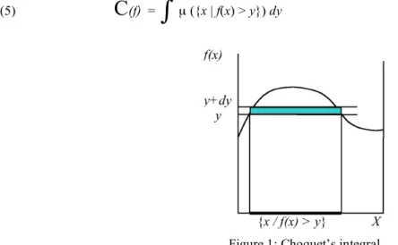
Since it involves only operators max and min, this integral is not appropriate for modelling synergy. Choquet’s integral of a measurable function f:X→[0,1] relative to a measure µ is defined as: (5)

C

∫

Figure 1: Choquet’s integral For example, in the case of a finite set X = {x₁, x₂, ... x_n} with: 0 ≤ f (x1) ≤ ... ≤ f(xn) ≤ 1 and Ai = {xi, ... xn}, we have:

C

i =1 n

!

Moreover, 1(A=B) being the "indicator function" which takes value 1 if A=B and 0 otherwise , we can write:

C

∫

A! X

"

µ (A) .

1

C

A! X

"

µ (A) . (

∫

1

If we denote gA(f) as the value of the expression

∫

1

the following manner:

C

A! X

"

µ(A) . gA(f)

Choquet’s integral involves the sum and the usual product as operators. It reduces to Lebesgue’s integral when µ is Lebesgue’s measure, and therefore extends it to possibly non additive measures. As a result of monotonicity, it is increasing with respect to the measure and to the integrand. Hence, Choquet’s integral can be used as an aggregation operator.

2.2.3. Principal applications of fuzzy integrals

Fuzzy integrals found an especially suitable field of application in the control of industrial processes (Sugeno, 1977). This approach then enabled fresh approaches to economic theory to be made on subjects such as non-additive probabilities, expected utility without additivity (Schmeidler, 1989), and the paradoxes relating to behaviour in the presence of risk (Wakker, 1990). More recently, they have been used as aggregation operators for the modelling of multicriteria choice, particularly in the case of problems of subjective evaluation and classification (Grabisch and Nicolas, 1994; Grabisch et al., 1995). With regard to the latter applications, fuzzy integrals exhibit the properties usually required from an aggregation operator whilst providing a very general framework for formalization.

The fuzzy integral approach means that the defects of classical operators can be compensated for (Grabisch et al., 1995). Including most other operators as particular cases, fuzzy integrals permit the detailed modelling of such features as:

• The redundancy through the specification of the weights on the criteria, but also on the groups of criteria. Taking into account the structuring effect makes possible to take interaction and the interdependency of criteria into account: µ is under-additive when the elements are redundant or mutually inhibiting; µ is additive for the independent elements; µ is over-additive when expressing synergy and reinforcement. • The compensatory effect: all degrees of compensation can be expressed by a continuous change from

minimum to maximum.

• The semantic underlying the aggregation operators.

2.3. Fuzzy Measure learning method (Casta and Bry, 1998)

Modelling through Choquet’s integral presupposes the construction of a measure which is relevant to the semantic of the problem. Since the measure is not a priori decomposable, it becomes necessary to define the value of 2n coefficients µ(A) where A ∈ P(X). We suggest an indirect econometric method for estimating the coefficients. Moreover, in cases where the structure of the interaction can be defined approximately, it is possible to reduce the combinatory part of the problem by restricting the analysis of the synergy to the interior of the useful subsets (see Casta and Bry, 1998). Determining fuzzy measures (that is to say 2n coefficients) brings us back to a problem for which many methods have been elaborated (Grabisch and Nicolas, 1994; Grabisch et al. 1995). We propose a specific method of indirect estimation on a learning sample made up of companies for which the firm’s overall evaluation and the individual value of each element in its patrimony are known. Let us consider I companies described by their overall value v and a set X of J real variables xj representing the individual value of each element in the assets. Let fi be the function assigning to every variable xj its value for

company i: f_i: xj ! "! x_ij. We are trying to determine a fuzzy measure µ in order to come as close as possible to the relationship:

∀i: C

Let A be a subset of variables and gA(fi) be the variable called generator relative to A and defined as:

i → g_A(fi) =

∫

1

∀ i vi =

A! X

"

µ(A) . g_A(fi) + ui

in which ui is a residual which must be globally minimized in the adjustment. It is possible to model this residual

as a random variable or, more simply, to restrict oneself to an empirical minimization of the ordinary least squares type . The model given below is linear with 2J _{parameters: the µ(A)’s for all the subsets A of variables x}j_.

The dependent variable is the value v; the explanatory variables are the generators corresponding to the subsets of X. A classical multiple regression provides the estimations of these parameters, that is to say the required measure. In practice, we shall consider the discrete case with a regular subdivision of the values:

y₀ = 0 , y₁ = dy , .... , y_n = n.dy and for each group A of variables xj, we compute the corresponding generator as:

g_{A(fi) = dy .}

_!

n h 0

1

µ(A B! )"µ( )A +µ( )B ⇔ synergy between A and B

µ(A B! )"µ( )A +µ( )B ⇔ mutual inhibition between A and B

It should be noted that the suggested model is linear with respect to the generators, but obviously non-linear in the variables xj. Moreover, the number of parameters only expresses the most general combination of

interactions between the xj. For a small number of variables xj, (up to 5 for example) the computation remains possible. The question is not only to compute the parameters, but also to interpret all the differences of the type

µ(A B! ) ( ( )" µ A +µ( ) )B . For a greater number of variables, one may consider either to start with a

preliminary Principal Components Analysis and adopt the first factors as new variables, or to restrict a priori the number of interactions considered.

2.4. Measure estimation

2.4.1. Numerical illustration

Consider a set of 35 companies evaluated globally (value V) as well as through a separate evaluation of three elements of the assets (A, B and C). Since the values A, B, C are integer numbers (ranging from 0 to 4), we have divided the value field into unit intervals dy = 1. Computing generators is very simple. For example, take company i=3 described in the third line of table 1, and let us represent its values for A, B and C:

0 1 2 3 4 A B C

Figure 2: Computation of the generator for company i = 3 {x | fi(x) > 3} = ∅

{x | fi(x) > 2} = {C} {x | fi(x) > 1} = {A,B,C} {x | fi(x) > 0} = {A,B,C}

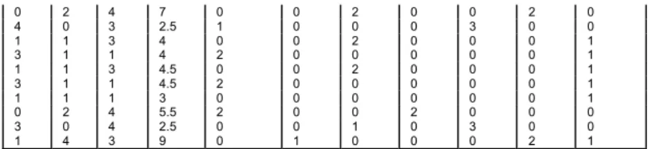
Hence we derive the value of the generators g{C}(i) = 1, g{A,B,C}(i) = 2, the other generators having a value of 0. For the whole sample of companies we have the following generators (Table 1):

A B C V _{g{A} g{B} g{C}} g

{A,B} g {A,C} g {B,C} g {A,B,C}

3 1 2 4 1 0 0 0 1 0 1 1 3 2 6 0 1 0 0 0 1 1 2 2 3 6.5 0 0 1 0 0 0 2 1 3 2 6.5 0 1 0 0 0 1 1 2 2 3 7 0 0 1 0 0 0 2 1 3 1 4.5 0 2 0 0 0 0 1 2 2 1 6 0 0 0 1 0 0 1 4 2 1 6.5 2 0 0 1 0 0 1 3 1 3 4.5 0 0 0 0 2 0 1 1 2 2 5.5 0 0 0 0 0 1 1 2 1 2 3.5 0 0 0 0 1 0 1 2 1 3 4 0 0 1 0 1 0 1 4 2 1 6 2 0 0 1 0 0 1 3 1 3 4 0 0 0 0 2 0 1 0 2 4 6 0 0 2 0 0 2 0 4 0 3 2 1 0 0 0 3 0 0 1 1 1 3.5 0 0 0 0 0 0 1 2 2 2 6.5 0 0 0 0 0 0 2 1 2 2 6 0 0 0 0 0 1 1 2 1 2 4 0 0 0 0 1 0 1 2 1 3 4.5 0 0 1 0 1 0 1 3 1 2 4.5 1 0 0 0 1 0 1 2 2 2 6 0 0 0 0 0 0 2 1 3 1 4 0 2 0 0 0 0 1 2 2 1 5 0 0 0 1 0 0 1

0 2 4 7 0 0 2 0 0 2 0 4 0 3 2.5 1 0 0 0 3 0 0 1 1 3 4 0 0 2 0 0 0 1 3 1 1 4 2 0 0 0 0 0 1 1 1 3 4.5 0 0 2 0 0 0 1 3 1 1 4.5 2 0 0 0 0 0 1 1 1 1 3 0 0 0 0 0 0 1 0 2 4 5.5 2 0 0 2 0 0 0 3 0 4 2.5 0 0 1 0 3 0 0 1 4 3 9 0 1 0 0 0 2 1

Table 1: Computation of generators for the whole sample

Then, by regressing the global value on the generators, we obtain (with an R2 _{of 0.96) the results displayed in} Table 2:

({A}) ({B}) ({C}) ({A,B}) ({A,C}) ({B,C}) ({A,B,C})

0,50 0,55 0,57 2,25 0,60 2,66 3,12

Table 2: Regression of the global value of the generators

The interpretation is simple in terms of structuring effects: each of the criteria A, B and C, taken individually, has more or less the same importance. But there is a strong synergy between A and B on one hand, and between B and C on the other; A and C partly inhibit each other (possible redundancy between the two). There is no synergy being the specific property of the 3 grouped criteria: µ({A,B,C}) is barely different from the sum µ({A,B}) +µ({C}), as well as from µ({B,C}) +µ({A}). The fact that it is superior to µ({A,C}) + µ({B}), denoting synergy between {A,C} and {B}, simply comes from the synergy already observed between A and B on one hand, and between C and B on the other hand.

2.4.2. Limiting a priori the combinatory effect of the interactions The extension principle:

Instead of considering the set P(A) of the A-subsets to define the measurement, we have only considered a limited number of these subsets , the measure µ on all the other subsets being defined univocally by an extension rule. The extension rule that naturally springs to mind is addition. Indeed, addition being equivalent to non-interaction, the set of all A-subsets on which µ is not a priori defined as additive is that of all interactions considered by the model.

Take for example a set of 6 variables: {a,b,c,d,e,f}. One can for instance restrict interactions to {b,c} and {e,f}. Measure µ will hence be defined through the following values: µ({a}), µ({b}), µ({c}), µ({d}), µ({e}), µ({f}), µ({b,c}), µ({e,f}). From these values, µ can be computed for any A-subset using the addition as extension rule. For instance, µ({a,b,c}) = µ({a})+µ({b,c}). Note that computing µ({a,b,c}) as µ({a}) +µ({b}) +µ({c}) would violate the assumption that b and c can interact.

We shall refer to all subsets corresponding to interactions considered by the model as kernels of measure µ . In the example above, there are 8 kernels. We shall consider that singletons (atoms of the measure) are kernels too. Taking a subset B, we shall say that a kernel N is B-maximal if and only if: N ⊂ B and there exists no other kernel N’ distinct from N and such that N ⊂ N’⊂ B .

The extension rule can then be stated accurately as follows: given any subset B, find a partition of B using only B-maximal kernels {N1, … , NL}, and compute µ(B) as µ(Nk)

k=

!

.

In the example above, there are only two ways to partition subset {a,b,c} using kernels: B = {a} ∪ {b} ∪ {c} and B = {a} ∪ {b,c}. The latter uses only B-maximal kernels, whereas the former does not.

We therefore see that if a subset B can be partitionned in more than one way using B-maximal kernels only and if the values of µ over the kernels are not constrained, the extension principle may lead to two distinct values of µ(B). So, in order for the extension rule to remain consistent, the set of kernels must fulfil certain conditions . The kernel set structure:

Let K be the set of kernels. K must abide by the following rule:

Rule R forbids the possibility that a subset B be partitionned in different ways using B-maximal kernels. Indeed, suppose subset B can be partitionned in two different ways using B-maximal kernels. Then, take any kernels N1 in partition 1 and N2 in partition 2 such that N1 ∩ N2 ≠ ! . If rule R holds, then N1 ∪ N2 ∈ K and either N1 = N2 or one of the two kernels is not B-maximal, which contradicts one of the hypotheses. Therefore, all intersecting kernels between partitions have to be identical, and then, partitions 1 and 2 have to be identical, which

contradicts the other hypothesis.

Conversely, the impossibility for any subset B to be partitionned in different ways using B-maximal kernels requires rule R to hold: supposing rule R does not hold, there exist distinct intersecting kernels N1 and N2 such that N1 ∪ N2 is not a kernel. Let B = N1 ∪ N2 , K1 be a B-maximal kernel containing N1 and K2 be a B-maximal kernel containing N2. B can then be partitionned in two different ways:

partition 1 = K1 ∪ partition of B\K1 using B-maximal kernels1 partition 2 = K2 ∪ partition of B\K2 using B-maximal kernels

There are two notable and extreme cases of structures complying with rule R:

1 – A partition hierarchy, i.e. a set of subsets between which only disjunction or inclusion relations hold, e.g.:

a b c d e f g

K = { {a},{b},{c},{d},{e},{f},{g},{d,e},{a,b,c},{d,e,f,g} } 2 – The set of all subsets of A.

Between these two extreme cases, various structures can be considered. Given, for instance, a partition of A into components, one can take every component, as well as all its subsets, as kernels:

a b c d e f g

K = { {a},{b},{c},{d},{e},{f},{g},{a,b},{b,c},{a,c},{d,e},{f,g},{a,b,c} } Integrating over the kernel structure:

This is achieved by simply computing the fuzzy integral with respect to the measure defined on the kernels and extended as stated above.

Measure estimation:

Estimating the measure µ on the kernels requires one extra step: the generators corresponding to the kernels have to be computed first. Recall that:

C

∫

_!

)

(

A

µ

1

∫

_!

_!

1

"

!

∫

1

1 _{where operator \ is the set difference.}

gN(f) =

!

∫

C

"

Take the following f, and kernel structure: f 0 1 2 3 4 a b c d e f a b c d e f K = { {a},{b},{c},{d},{e},{f},{a,b},{a,b,c},{d,e},{d,f},{e,f},{d,e,f} } We must examine, for y going from 0 to 4, every subset B = {x / f(x) > y}. We get:

y = 0 → B = {a,b,c,d,e,f} ; y = 1 → B = {a,b,c,d,e} y = 2 → B = {b,d,e} ; y = 3 → B = {d} y = 4 → B = ∅

Let us consider the B-maximality of kernel {d,e} with respect to each of these subsets. Kernel {d,e} appears to be B-maximal for B = {a,b,c,d,e} and for B = {b,d,e}. Hence, we draw: g{d,e}(f) = 1+1=2.

Once every kernel generator has been computed, we can proceed to the least squares step of the learning procedure, just as in § 2.4.

============ Conclusion:

After reviewing the possibilities offered by fuzzy integrals, we have observed that there exist many potential fields of application in finance for this family of operators. They enable the effects of micro-structure, synergy and redundancy, which are opaque in linear models, to be analysed in detail. There is a price to be paid for this sophistication in terms of computational complexity. However, we have tried to show that these techniques allow to limit the purely combinatory effects which appear at the learning stage of the methodology.

8.1. REFERENCES

Abdel-Magid M.F.: "Toward a better understanding of the role of measurement in accounting", The Accounting Review, 1979, april, vol. 54, n°2, 346-357.

Bry X., Casta J.F.: "Measurement, imprecision and uncertainty in financial accounting", Fuzzy Economic Review, 1995, november, 43-70.

Casta J.F.: "Le nombre et son ombre. Mesure, imprécision et incertitude en comptabilité", in Annales du Management, XIIèmes Journées Nationales des IAE, Montpellier, 1994, 78-100.

CastaJ.F., Bry X.: "Synergy, financial assessment and fuzzy integrals", in Proceedings of IVth Meeting of the International Society for Fuzzy Management and Economy (SIGEF), Santiago de Cuba, 1998, vol. II, 17-42.

Casta J.F., Lesage C.: Accounting and Controlling in Uncertainty : concepts, techniques and methodology, in Handbook of Management under Uncertainty, J. Gil-Aluja(ed.), Kluwer Academic Publishers, Dordrecht, 2001. Choquet G.: "Théorie des capacités", Annales de l'Institut Fourier, 1953, n°5, 131-295.

Ellerman D.P.: "Double–entry multidimensional accounting", Omega, International Journal of Management Science, 1986, vol. 14, n°1, 13-22.

Grabisch M.: "Fuzzy integral in multicriteria decision making", Fuzzy Sets and Systems, 1995, n°69, 279-298. Grabisch M., Nguyen H.T., Wakker E.A.: Fundamentals of uncertainty calculi with applications to fuzzy inference, Kluwer Academic Publishers, Dordrecht, 1995.

Grabisch M., Nicolas J.M.: "Classification by Fuzzy Integral: Performance and Tests", Fuzzy sets and systems, 1994, n°65, 255-271.

Ijiri Y.: The foundations of accounting measurement: a mathematical, economic and behavioral inquiry, Prentice Hall, Englewood Cliffs, 1967.

Ijiri Y.: The theory of accounting measurement, Studies in Accounting Research, n°10, American Accounting Association, 1975.

de Korvin A.: "Uncertainty methods in accounting: a methodological overview", in Seigel P.H., de Korvin A., Omer K. (eds): Applications of fuzzy sets and the theory of evidence to accounting, JAI Press, Stamford, Conn., 1995, 3-18.

March J.G.: "Ambiguity and accounting: the elusive link between information and decision making", Accounting, Organizations and Society, 1987, vol. 12, n°2, 153-168.

Mattessich R.: Accounting and analytical methods, Richard D. Irwin, Inc, 1964.

Morgenstern O.: On the accuracy of economic observations, Princeton University Press, 1950.

Schmeidler D.: "Subjective probability and expected utility without additivity", Econometrica, 1989, vol. 57, n°3, 571-587.

Sterling R.R.: Theory of the measurement ot enterprise income, The University Press of Kansas, 1970. Stevens S.S.: "Mathematical measurement and psychophysics", in Handbook of Experimental Psychology, Stevens (ed.), John Wiley and Sons, New-York, 1951, 1-49.

Stevens S.S.: "Measurement, psychophysics and utility", in Measurement: Definitions and Theories, C.W. Churman and P. Ratoosh (eds.), John Wiley and Sons, New-York, 1959, 18-63.

Sugeno M.: "Fuzzy measures and fuzzy integrals: a survey", in Fuzzy Automata and Decision Processes, Gupta, Saridis, Gaines (eds.), 1977, 89-102.

Tippett M.: "The axioms of accounting measurement", Accounting and Business Research, 1978, autumn, 266-278.

Vickrey D.W.: "Is accounting a measurement discipline ?", The Accounting Review, 1970, october, vol. 45, 731-742.

Wakker P.: "A behavioral foundation for fuzzy measures", Fuzzy Sets and Systems, 1990, n°37, 327-350. Willett R.J.: "An axiomatic theory of accounting measurement", Accounting and Business Research, 1987, spring, n° 66, 155-171.

Zebda A., "The problem of ambiguity and vagueness in accounting and auditing", Behavioral Research in Accounting, 1991, vol. 3, 117-145.