A stochastic movement model reproduces patterns of site fidelity and long-distance dispersal in a population of Fowler’s toads (Anaxyrus fowleri)

A stochastic movement model reproduces patterns of site

fidelity and long-distance dispersal in a population of

Fowler’s Toads (Anaxyrus fowleri)

Philippe Marchand*, National Socio-Environmental Synthesis Center (SESYNC), Annapolis, MD 21401, United States.

Morgan Boenke, Department of Biology, McGill University, Montreal, Quebec H3A 1B1, Canada.

David M. Green, Redpath Museum, McGill University, Montreal, Quebec H3A 0C4, Canada.

* Corresponding author: marchand.philippe@gmail.com. ORCID: 0000-0001-6717-0475.

1 2 3 4 5 6 7 8 9 10 11 12 13 4 5 6 7 8 9 10 11 12 13 14 15 16 17 18 19 20 21 22 23 24 25 26 27 28 29 30 31 32 33 34 35 36 37 38 39 40 41 42 43 44 45 46 47 48 49 50 51 52 53 54

Abstract

Although amphibians typically exhibit high site fidelity and low dispersal, they do undertake rare, long-distance movements. The factors influencing these events remain poorly understood, partly because amphibian spring movements tend to radiate from breeding sites and the animals are often difficult to locate at other times of the year. In this study, we investigate whether these movement patterns can be reproduced by a parsimonious model where foraging steps follow a heavy-tailed, Lévy alpha-stable distribution and individuals may either return to a previous refuge site or establish a new one. We consider three versions of the return behaviour: (1) a distance-independent probability of return to any previous refuge; (2) constant probability of return to the nearest refuge; or (3) a distance-dependent probability of return to each refuge. Using approximate Bayesian computation, we fit each version of the model to radiotracking data from a population of Fowler’s Toads, which inhabits a linear sand dune habitat on the north shore of Lake Erie in Ontario, Canada. Only the model with distance-independent, random returns provides a good fit of the inter-refuge distance distribution and the number of refuges visited per toad. Our results suggest that while toads occasionally forage over long distances, the

establishment of new refuges is not driven by the minimization of energy expenditure.

Keywords: amphibian; animal movement; approximate Bayesian computation; foraging; Lévy walk; radiotracking 14 15 16 17 18 19 20 21 22 23 24 25 26 27 28 29 30 31 32 33 61 62 63 64 65 66 67 68 69 70 71 72 73 74 75 76 77 78 79 80 81 82 83 84 85 86 87 88 89 90 91 92 93 94 95 96 97 98 99 100 101 102 103 104 105 106 107 108 109 110

1. Introduction

The movements that individual animals undertake to go from place to place are

fundamental to virtually every aspect of animal ecology and behaviour. How small movements of animals at daily or hourly scales result in such larger phenomena as home-ranges, dispersal and migrations at seasonal, annual or life-time scales, however, remains a difficult problem to understand. It has commonly been observed that a high-frequency of short-distance movements combined with rare, long-distance movement events results in a movement step size distribution that is strongly leptokurtic, with a sharper peak and longer tails than expected of a normal distribution, and possibly heavy-tailed, i.e. with the long-distance probability tail extending past that of an exponential distribution (e.g., Cecala et al., 2009; Gomez and Zamora, 1999; Morales, 2002; Paradis et al., 1998; Skalski and Gilliam, 2000). Such heavy-tailed distributions in animal movement may be consistent with the Lévy flight foraging hypothesis (Viswanathan et al., 1999), according to which optimal search patterns follow a power-law distribution of step sizes, with the frequency of steps proportional to some inverse power of their length. However, tests of this hypothesis have been the subject of numerous statistical challenges (Edwards, 2011).

In actuality, animal movement is not scale-free and must be constrained by biological limits, so that the power-law distribution can only hold within a certain range of step sizes (Benhamou, 2007). Over the longer time scales that encompass multiple individual movements, such as may occur during foraging or dispersal behaviours, movement distances may also depend on the animal’s memory and “cognitive map” of the environment, features that are poorly

represented in movement models based on independent steps (Gautestad and Mysterud, 2013). More complex models that can accommodate both specific movement rules and memory effects

34 35 36 37 38 39 40 41 42 43 44 45 46 47 48 49 50 51 52 53 54 55 116 117 118 119 120 121 122 123 124 125 126 127 128 129 130 131 132 133 134 135 136 137 138 139 140 141 142 143 144 145 146 147 148 149 150 151 152 153 154 155 156 157 158 159 160 161 162 163 164 165 166

may be required, but their outcomes may not be expressible in terms of analytical likelihood functions.

Although the absence of a likelihood function previously precluded formal statistical analysis, computational and statistical advances in the last 20 years have made it possible to derive inferences from simulation-based models (Hartig et al., 2011). Approximate Bayesian computation (ABC) is a simulation-based inference method originally developed in the field of population genetics, wherein the large number of possible genetic histories and intermediate states leading to a given outcome make explicit likelihood calculations intractable (Beaumont et al., 2002). Since analogous challenges, i.e. path dependence and a large number of unobserved intermediate states, are also encountered in the study of animal movement, ABC provides a flexible mean to test foraging and dispersal behaviour models with empirical data (Marchand et al., 2015).

Anuran amphibians, although they have generally been considered poor dispersers relative to larger, more vagile terrestrial vertebrates, can be valuable subjects for testing models of animal movement. Individuals may show a high level of site fidelity yet mark-recapture studies have also shown that anurans will undertake relatively rare long-distance movements of up to a few km in a matter of days, or as far as 35km over the course of a season (Smith and Green, 2005, 2006). Whether site fidelity is advantageous should depend on the tradeoff between the benefit of a known location relative to the cost of returning to that location (Wells, 2007). As many amphibian species make use of refuge sites as part of their daily activity cycles, this makes discretizing movement simpler as time periods between movement steps are more or less standardized and biologically meaningful. Nevertheless, locating individual anurans outside

56 57 58 59 60 61 62 63 64 65 66 67 68 69 70 71 72 73 74 75 76 77 173 174 175 176 177 178 179 180 181 182 183 184 185 186 187 188 189 190 191 192 193 194 195 196 197 198 199 200 201 202 203 204 205 206 207 208 209 210 211 212 213 214 215 216 217 218 219 220 221 222

of the breeding season can be difficult with many species as they tend to be mostly nocturnal foragers that hide during the daytime. Moreover, the small size of most species precludes the use of GPS satellite telemetry methods that can provide long-term, high-resolution movement time-series for larger terrestrial animals (Wikelski et al., 2007). Both of these difficulties can be overcome, however, with the appropriate model species.

In this study, we develop a parsimonious model that describes both site fidelity and long-distance movements, and apply this model to the movements of Fowler’s Toads (Anaxyrus fowleri) in a population inhabiting a linear sand dune habitat on the north shore of Lake Erie in Ontario, Canada. In this environment, adult Fowler’s Toads are readily locatable as they forage on the beaches at night (Greenberg and Green, 2013). Previous capture-mark-recapture data (Smith and Green 2005, 2006) have established and quantified the heavy-tailed movement distribution curve of these toads. The toads can also be fitted with small radio-transmitters (Boenke, 2011), which allow them to be tracked to their daytime hiding places in the sand dunes fronting the beaches. Based on this radiotracking data, we use ABC to estimate the parameters of the movement model, including the scale and shape of a Lévy-stable distribution of movement steps and the probability of returning to a known refuge rather than establishing a new one.

To assess the importance of energy constraints on movement, we compare the relative fit of three versions of the return step: (1) toads return to a randomly selected previous refuge, independent of distance; (2) they return to the nearest refuge from their current location; or (3) the probability of return to any previous refuge is a decreasing function of the distance to that refuge. We hypothesize that either of the last two models would provide a better fit if minimizing energy expenditure were the primary factor determining refuge choice.

78 79 80 81 82 83 84 85 86 87 88 89 90 91 92 93 94 95 96 97 98 99 228 229 230 231 232 233 234 235 236 237 238 239 240 241 242 243 244 245 246 247 248 249 250 251 252 253 254 255 256 257 258 259 260 261 262 263 264 265 266 267 268 269 270 271 272 273 274 275 276 277 278

2. Methods

2.1. Study site and population

We studied the movement ecology of Fowler’s Toads at Long Point in Ontario, Canada, along the beaches of Long Point Provincial Park and the Long Point National Wildlife Area Thoroughfare Point Unit (UTM zone 17 N: 550700 – 553000 Easting, 4713615 – 4714200 Northing; NAD 83 Datum). Although the dune ecosystems along the north shore of Lake Erie are highly dynamic (Gelinas and Quigley, 1973; Stenson, 1993), human disturbance at this site is minimal and movement by toads not constrained either by lack of suitable habitat or by lack of connectivity between habitat patches (Smith and Green, 2005, 2006). The toads generally take refuge in the sand dunes fronting the beach during the day and emerge to forage for invertebrate prey along the lakeshore at night.

2.2. Stochastic movement model

To reflect both the high rate of apparent site fidelity and the heavy-tailed distribution of dispersal steps present in the previous mark-recapture data (Smith and Green, 2006), we used a variant of the multiscaled random walk (MRW) model proposed by Gautestad and Mysterud (2005). The MRW is based on a power-law step length distribution, but differs from a classic Lévy flight by allowing a certain frequency of return steps, wherein the individual revisits a location chosen at random from previous points in the walk. As each successive visit to a

location increases its effective weight for future return steps, the MRW model allows home range patterns to emerge without the need to specify an ad hoc homing process.

100 101 102 103 104 105 106 107 108 109 110 111 112 113 114 115 116 117 118 119 120 121 285 286 287 288 289 290 291 292 293 294 295 296 297 298 299 300 301 302 303 304 305 306 307 308 309 310 311 312 313 314 315 316 317 318 319 320 321 322 323 324 325 326 327 328 329 330 331 332 333 334

In our model, we assumed that return steps only occurred at the end of the nighttime foraging path, when the toad is at a position Δxn away from the previous day’s refuge site. At this point, the toad either takes refuge at its current position or returns to a known refuge site.

2.2.1. Return steps

Our three model versions differ in how they describe the return behaviour:

Model 1 (random return): The probability of return is constant (pret = p0), and the toad selects a

refuge at random from all the previous days’ refuges. As in Gautestad and Mysterud’s model, multiple visits to a refuge increase its “weight” for future return steps.

Model 2 (nearest return): The probability of return is constant (pret = p0), but the toad always

returns to the nearest refuge.

Model 3 (distance-based return probability): The probability of returning to a given site decays exponentially with the distance di to that refuge:

p_ret(i)=p0e

− di

d0 , (1)

where d0 is a characteristic distance to be estimated along with p0. The probability of not

returning to any previous site is the product of the complements of the pret(i) :

1− pret=

∏

(

)

In the case of a return event, the probability of each refuge being chosen is given by: P

(

|

)

∑

With an additional parameter, the third model allowed us to consider intermediate cases of distance-dependence. As the characteristic distance d0 decreases, it becomes increasingly

122 123 124 125 126 127 128 129 130 131 132 133 134 135 136 137 138 139 140 141 142 340 341 342 343 344 345 346 347 348 349 350 351 352 353 354 355 356 357 358 359 360 361 362 363 364 365 366 367 368 369 370 371 372 373 374 375 376 377 378 379 380 381 382 383 384 385 386 387 388 389 390

likely that the toad will choose the nearest refuge; yet the outcome differs from that of model 2, since the probability of return is not constant but decreases with distance. In the limit where d0 is

very large, pret(i) = p0 and all previous sites have the same probability of return. Contrary to model

1, however, the probability of returning to any site is not constant but increases with R (as a consequence of Eq. 2). Moreover, since model 3 considers distinct refuge sites, multiple visits to the same refuge do not increase its probability weight.

2.2.2. Overnight displacement

The net overnight displacement, Δxn, in the model followed a symmetric, zero-centered

stable (a.k.a. Lévy alpha-stable) distribution, S(α, ), with stability parameter α (0 < α ≤ 2) and scale parameter  > 0. With α = 2, the stable distribution reduces to a normal law, whereas decreasing values of α produced increasingly leptokurtic (i.e. heavy-tailed) distributions,

including the Cauchy distribution (α = 1) as a special case (Uchaikin and Zolotarev, 1999). For α < 2, the tails of the probability density followed a power law decay with exponent −(1 + α).

Although there is no closed form of the stable probability density for arbitrary α, random draws from S(α, ) can be generated by the CMS algorithm (Chambers et al. 1976):

S=γ sin αU

(

)

[

((1− α

)

)

]

where U is a uniformly distributed angle in (−, ) and W has a standard exponential distribution.

A key property of the stable distribution is that the sum of stable random variables is also stable; in particular, the sum of N independent variables distributed as S(α, ) is stable with the

143 144 145 146 147 148 149 150 151 152 153 154 155 156 157 158 159 160 161 162 163 397 398 399 400 401 402 403 404 405 406 407 408 409 410 411 412 413 414 415 416 417 418 419 420 421 422 423 424 425 426 427 428 429 430 431 432 433 434 435 436 437 438 439 440 441 442 443 444 445 446

same stability parameter α and a scale N = N1/α . Furthermore, the generalized central limit

theorem of Gnedenko and Kolmogorov (1954) shows that the sum of independent variables following a common distribution with asymptotic power-law tail converges to a stable distribution.

Given these properties, our assumption that Δxn has a stable distribution was robust to

differences in the small-scale foraging behaviour. For example, while foraging steps are probably correlated on a short-term scale, as long as there is some intermediate time scale where

successive displacements can be modelled as independent and following a heavy-tailed (power-law) distribution, the stable distribution will be a reasonable approximation of net displacement.

2.3. Model fitting with approximate Bayesian computation

We fitted our model by approximate Bayesian computation (ABC) using the ABC-rejection algorithm, as implemented in the ‘abc’ package (Csilléry et al., 2012) in R (R Core Team, 2016). Consider a simulation model that takes an input parameter vector  and outputs a vector of summary statistics (S) calculated from the simulation outcome. Given a set of  vectors, drawn from the parameters’ prior distributions, and a corresponding set of simulation outputs S(), ABC-rejection simply selects a subset of  for which the output statistics are close to those of the observed data D, i.e. where d[S(), S(D)] <  for a chosen distance function d and tolerance level . The selected subset approximates the joint posterior distribution of . The approximation accuracy can be further improved by fitting a local-linear regression model of  vs. S() and using that empirical model to correct each  towards the value it would have at S(D) (Beaumont et al., 2002). 164 165 166 167 168 169 170 171 172 173 174 175 176 177 178 179 180 181 182 183 184 185 452 453 454 455 456 457 458 459 460 461 462 463 464 465 466 467 468 469 470 471 472 473 474 475 476 477 478 479 480 481 482 483 484 485 486 487 488 489 490 491 492 493 494 495 496 497 498 499 500 501 502

The ABC-rejection algorithm can be naturally extended to the problem of model selection by treating the choice of model as a discrete parameter (Toni et al., 2009). If the number of simulations run under each model is proportional to its prior probability, then the representation of a model among the simulations retained following the rejection step is an estimate of its posterior probability. As in the parameter estimation case, the approximation can be improved by fitting a regression of the discrete model probabilities, i.e. a multinomial logistic regression, as a function of the summary statistics in the vicinity of the observed statistics (Beaumont, 2008).

The main drawback of ABC-rejection is the high number of simulations necessary to get a sufficient number of results in the vicinity of the data. Alternative ABC algorithms use Markov chain Monte Carlo or sequential Monte Carlo (a.k.a. particle filter) methods to gradually

concentrate the sampling effort in the areas of high-agreement between simulated and observed statistics (Marjoram et al., 2003; Sisson et al., 2007). Yet, ABC-rejection has the advantage of decoupling the simulation and estimation steps, which allows the entire set of simulations to be run ahead of time and, possibly, in parallel on a high-performance computing cluster. Multiple estimations can then be performed from this set of simulation outputs, which is especially helpful when performing cross-validation.

2.3.1. Prior distributions and summary statistics

Our results were based on 10,000 simulations of each version of the stochastic model. For each simulation, we drew parameters from the following uniform prior distributions: α ~ U(1, 2),  ~ U(10m, 100m), p0 ~ U(0, 1) and (for model 3 only) d0 ~ U(20m, 2000m). To match the size

and structure of the observed dataset, we simulated the movement of 66 toads over 63 days, then

186 187 188 189 190 191 192 193 194 195 196 197 198 199 200 201 202 203 204 205 206 207 509 510 511 512 513 514 515 516 517 518 519 520 521 522 523 524 525 526 527 528 529 530 531 532 533 534 535 536 537 538 539 540 541 542 543 544 545 546 547 548 549 550 551 552 553 554 555 556 557 558

subset the results to keep only the (Toad, Day) observation points present in the data. For each of four different time lags (1, 2, 4 and 8 days), we calculated three statistics over all pairs of points with the same toad and the corresponding time lag: (1) the frequency of returns (defined as |Δx|< 10m), as well as (2) the mean and (3) standard deviation of log (Δx)2 _{for non-returns, over all}

pairs of points with the same toad and corresponding time lag. We chose these 12 summary statistics as well as the 10m distance threshold to capture the key characteristics of the empirical distribution of relocation distances at multiple time scales (see section 3.1 and Fig. 1). We used the Euclidean distance (sum of squared differences) to compare this vector of summary statistics to the corresponding statistics of the radiotracking data.

2.3.2. Cross-validation

We used the ‘abc’ package’s cross-validation feature to verify the identifiability of our model, i.e. determining whether the size of the dataset and the chosen summary statistics are sufficient to estimate the parameters of interest for each model version, and distinguish the outcome of the alternate model versions. We also used cross-validation to choose an optimal tolerance rate, which is the fraction of best-fitting simulations to keep for estimating the posterior distribution.

For the parameter estimation problem, cross-validation was performed separately for each model version. Taking one of the simulation results as the “data”, we applied ABC to estimate the true parameters of that simulation based on the remainder of the simulation results. We repeated this process for 100 sampled simulation results and four different tolerance rates (0.5%, 1%, 5% and 10%). The cross-validation accuracy was quantified using the relative

208 209 210 211 212 213 214 215 216 217 218 219 220 221 222 223 224 225 226 227 228 229 564 565 566 567 568 569 570 571 572 573 574 575 576 577 578 579 580 581 582 583 584 585 586 587 588 589 590 591 592 593 594 595 596 597 598 599 600 601 602 603 604 605 606 607 608 609 610 611 612 613 614

estimation error, defined as the mean square difference between estimated and true parameter values divided by the variance of the true values over the 100 sampled simulations.

For the model selection problem, cross-validation consisted in taking one simulation output as the data and applying ABC to the remaining 29,999 simulation results (combined from all three models) to estimate the posterior probabilities of each model version. We repeated this process for 100 sampled simulations per model version, using the same tolerance rates as above. Model selection accuracy is quantified by the misclassification rate: the fraction of cases where the model version with the highest posterior probability differed from the true model.

2.3.3. Parameter estimates and model selection

We estimated the posterior distribution of each parameter via ABC-rejection, using the tolerance rate selected by cross-validation and applying the local-linear regression correction of Beaumont et al. (2002). For the regression correction, we applied a logit transformation to the stability parameter (α) to keep the inferred values within the (1, 2) bounds, and a log

transformation to d0 to constrain its range to positive values. Parameters were estimated

separately for the three versions of the model.

To compare the fit of the different model versions, we first estimated the posterior probabilities of the three models by ABC-rejection, followed by multinomial logistic regression of model probabilities in the vicinity of the observed summary statistics (Beaumont 2008). We then verified that simulation outputs from the fitted version of each model (with parameters drawn from their posterior distribution) could reproduce the observed summary statistics.

230 231 232 233 234 235 236 237 238 239 240 241 242 243 244 245 246 247 248 249 250 621 622 623 624 625 626 627 628 629 630 631 632 633 634 635 636 637 638 639 640 641 642 643 644 645 646 647 648 649 650 651 652 653 654 655 656 657 658 659 660 661 662 663 664 665 666 667 668 669 670

As an additional posterior predictive check, we compared the number of distinct refuge sites in the simulated and observed datasets. In practice, we defined this quantity as the number of clusters obtained at a distance threshold of 10m, when performing hierarchical clustering of the point locations using the linkage method (‘hclust’ function in R). The complete-linkage criterion ensures that each pair of points in the cluster is separated by no more than the specified distance threshold.

2.4. Radiotracking data

We collected radiotracking data on Fowler’s Toads at our study site during mid-June to late August of 2009 and 2010 (Boenke, 2011). Toads were captured opportunistically while they were foraging on the beach, and outfitted with either Holohil BD-2 (in 2009) or BD-2N (in 2010) radiotransmitters, which were attached to the toad via a filament covered in plastic tubing

(following Bartelt and Peterson, 2000). The total weight of the transmitter and harness (ca. 2 g) constituted ~5% of the typical adult toad weight, and in no case exceeded 10% of the

individual’s weight, as recommended by Rowley and Alford (2007). Toads were tracked with an HR2600 Osprey Receiver (H.A.B.I.T. Research, Victoria, BC, Canada) and Yagi 3-element antenna. Upon finding each toad, its position was recorded with a Magellan Mobile Mapper 6 GPS unit (Magellan Navigation, Inc., Santa Clara, CA, USA). The location of each tracked toad was recorded at least once per night (active foraging) and once per day (resting in refuge) but we only used the daytime locations in the present study. The number of consecutive days in a

tracking bout varied by toad, as some individuals shed their transmitter, or else it had to be removed to alleviate skin irritation. Since individuals were identified by toe clipping or

251 252 253 254 255 256 257 258 259 260 261 262 263 264 265 266 267 268 269 270 271 272 676 677 678 679 680 681 682 683 684 685 686 687 688 689 690 691 692 693 694 695 696 697 698 699 700 701 702 703 704 705 706 707 708 709 710 711 712 713 714 715 716 717 718 719 720 721 722 723 724 725 726

distinctive marks from digital photographs, toads that lost their transmitter could sometimes be retrieved, allowing multiple tracking bouts per toad (Boenke, 2011). All procedures with animals were conducted under McGill University Animal Use Protocol No. 4569.

The position of toads’ daytime refuges relative to the shore is governed by tradeoffs between wave avoidance, predator avoidance, elevation and proximity to water (Boenke, 2011). In contrast, movement along the shoreline is unconstrained, meaning that dispersal occurs mostly along a single dimension. For this reason, we projected all refuge locations on a single axis, obtained by linear regression of the two-dimensional coordinates, and only modeled this one-dimensional component of toad movement.

2.5. Source code and data access

The dataset used for this study and the R code for all simulation and analyses can be downloaded from GitHub: http://github.com/pmarchand1/fowlers-toad-move/.

3. Results

3.1. Empirical distribution of relocation distances

The radio-tracking dataset included 66 toads, with between 2 and 30 daytime points recorded, for a mean of 12 locations per toad per season.

When shown on a logarithmic scale (Fig. 1), the distribution of distances between daytime refuges of a toad was characterized by a symmetric peak combined with an inflated number of low-distance events. Given the GPS margin of error of 3 – 5m per point, distances of less than 10m could not be measured reliably (Boenke, 2011). Therefore, the excess probability

273 274 275 276 277 278 279 280 281 282 283 284 285 286 287 288 289 290 291 292 293 294 733 734 735 736 737 738 739 740 741 742 743 744 745 746 747 748 749 750 751 752 753 754 755 756 757 758 759 760 761 762 763 764 765 766 767 768 769 770 771 772 773 774 775 776 777 778 779 780 781 782

in that part of the distribution would be consistent with toads returning to previous sites. In contrast with the expectations of a random walk model, where the whole distribution would shift to larger distances as the time step increases, the peak of relocation distances varied little

between time lags of 1 to 8 days. Instead, longer time lags increased the total probability on the high end of the distribution as the fraction of short-distance (or return) events decreased.

3.2. Approximate Bayesian computation 3.2.1 Cross-validation

With the exception of d0 in model 3 (see below), the cross-validation results (Table S1 in

the supplementary data) showed a good agreement between the true values of the parameters and their posterior median estimated via ABC. Overall, the relative estimation error was minimized with a 5% tolerance level; the supplementary Fig. S1 shows how the estimated and true values compare across all parameters at that tolerance level. For all three model versions, the relative error was higher for α (10% to 14%) than for  (around 7%) or p0 (1% to 5%). Since α

determines the power-law tail of the stable distribution, its value is sensitive to rare, long-distance events, which could explain the higher estimation variance. The characteristic long-distance d0 had the highest estimation error, at over 60% of the prior range. Therefore, this parameter

might only be identifiable with a larger dataset.

The ABC model selection algorithm could discriminate well between Model 2 and either other version. However, 35% of the Model 1 runs were misidentified as Model 3 and 23% of Model 3 runs were misidentified as Model 1 (Table 1). This is consistent with the behaviour of Model 3 approaching random returns in the limit of high d0; while there are still differences

295 296 297 298 299 300 301 302 303 304 305 306 307 308 309 310 311 312 313 314 315 316 788 789 790 791 792 793 794 795 796 797 798 799 800 801 802 803 804 805 806 807 808 809 810 811 812 813 814 815 816 817 818 819 820 821 822 823 824 825 826 827 828 829 830 831 832 833 834 835 836 837 838

between the two models in that limit, they might not be detectable with the chosen summary statistics.

3.2.2. Parameter estimation

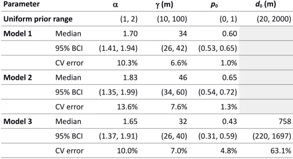
The posterior median and 95% Bayesian credible interval for all parameter estimates are shown in Table 2. The estimates of the stable distribution parameters were similar for Model 1 (α = 1.7,  = 34 m) and Model 3 (α = 1.65,  = 32 m), whereas both values were higher for Model 2 (α = 1.83,  = 46 m).

The estimated values of α suggest a power-law tail with an exponent between −2.6 and −2.8. The estimates of α could be biased upwards, however, since long-distance dispersal events are more likely to take toads outside of the tracking range. That is, the power-law tail could extend further than inferred from the data.

As expected based on the poor cross-validation results, the estimate of d0 in model 3 has a

very wide credible interval (220 to 1697 m). In comparison, the largest distance between any two observations of the same toad in the dataset was 1198 m, and only 4 out of 66 toads visited locations more than 350 m apart. Most of the posterior distribution thus lies in the high d0 range

where refuge choice is not primarily constrained by distance. Note that the estimates of p0 in

Model 3 (0.43) and Model 1 (0.60) are not directly comparable even in the distance-independent case, since the actual probability of return in Model 3 increases with the number of visited refuges (see section 2.2).

We verified that our posterior parameter estimates did not significantly change when performing additional simulations beyond the current 10,000 per model version (Fig. S2 in the supplementary data). 317 318 319 320 321 322 323 324 325 326 327 328 329 330 331 332 333 334 335 336 337 338 845 846 847 848 849 850 851 852 853 854 855 856 857 858 859 860 861 862 863 864 865 866 867 868 869 870 871 872 873 874 875 876 877 878 879 880 881 882 883 884 885 886 887 888 889 890 891 892 893 894

3.2.3. Model selection

The ABC model selection process resulted in posterior probabilities of 15% for Model 1 (random return), 0% for Model 2 (nearest return) and 85% for Model 3 (distance-dependent return probability). Given the high probability of misclassification between Model 1 and 3 (Table 1) and the difference in complexity between the two models (3 versus 4 adjustable parameters), this result alone does not provide strong evidence of a better fit for Model 3.

The comparison of observed and simulated summary statistics from the three models, with simulation parameters drawn from their respective posterior distribution, shows that Model 2 is too dispersive. That is, the mean log distance increases – and the probability of return decreases – too rapidly with greater time lags. In contrast, the range of simulated results from Models 1 and 3 is consistent with the observed statistics at all time lags (Fig. 2).

Finally, we computed the number of distinct refuge sites, defined in section 2.3 as clusters of points with diameter less than 10m, for each toad in both the empirical data and the output of each simulation model (with parameters drawn from their posterior distribution). This quantity is strongly dependent on the number of observations by individual; our results show that this relationship can be well approximated by a linear regression on a log-log plot (Fig. 3). Note that the simulation results show less variance as they represent the average of 500 simulated paths by toad. This number of refuges statistic, which wasn’t directly used in fitting the parameters of each model, shows a better fit for Model 1: the 95% confidence intervals of the regression lines for observed and simulated points overlap. Model 3, in contrast, results in too few distinct refuges for toads with many observations. This may be due to the functional form of

339 340 341 342 343 344 345 346 347 348 349 350 351 352 353 354 355 356 357 358 359 900 901 902 903 904 905 906 907 908 909 910 911 912 913 914 915 916 917 918 919 920 921 922 923 924 925 926 927 928 929 930 931 932 933 934 935 936 937 938 939 940 941 942 943 944 945 946 947 948 949 950

the probability of return in this model (Eq. 2), which increases with the number of distinct refuges already visited.

4. Discussion

In the analysis above, we showed that a parsimonious model of foraging behaviour (our Model 1) successfully reproduced the main patterns of refuge site fidelity and relocation among a population of Fowler’s Toads. The model assumed that the net displacements of toads during nighttime foraging follows a heavy-tailed, Lévy-stable distribution, and that toads may either take refuge at the end of their foraging path, or return to a random refuge among those previously visited.

The assumption that toads returning to a previous refuge choose one at random may seem unrealistic. Yet it fit the data better than two alternative models we tested, where the probability of return and/or the choice of refuge were distance-dependent. It might be that movement cost is only one of many factors determining refuge selection, along with slope, elevation and

vegetation cover of potential refuge sites (Boenke, 2011). Without knowing the spatial structure of these microhabitat variables along the beach length, it is difficult to determine how they could affect the movement statistics. Even if additional environmental data were available, the size of the tracking dataset (individuals and locations per individual) would also set a limit to the complexity of verifiable models: the very diffuse posterior distribution for the characteristic distance d0 in model 3 provides a good example of this problem.

Even for this simple model, this study illustrates the power and flexibility of approximate Bayesian computation for the calibration and testing of mechanistic movement models from field

360 361 362 363 364 365 366 367 368 369 370 371 372 373 374 375 376 377 378 379 380 381 957 958 959 960 961 962 963 964 965 966 967 968 969 970 971 972 973 974 975 976 977 978 979 980 981 982 983 984 985 986 987 988 989 990 991 992 993 994 995 996 997 998 999 1000 1001 1002 1003 1004 1005 1006

data. In particular, ABC doesn’t require the stochastic process of interest to have a known analytical likelihood, and it can easily accommodate gaps in observations (by subsetting the simulated data) as well as sources of error and censoring. In this study, we took into account the unreliability of GPS measurements at short distances, and if we had an independent measure of long-distance censoring, that effect could have been included as well.

Our results indicate that long-term movement patterns, such as dispersal, may be

profoundly affected by small-scale micro-habitat choices and day-to-day movement. Sand dunes and beaches are highly dynamic environments that are strongly affected by both weather

conditions and waves. The large temporal variation in habitat quality, combined with a relatively lower spatial variability in the direction parallel to the shore, matches conditions that have been found to favor heavy-tailed movement patterns (Lowe, 2009). Temporal habitat variability can also contribute to the decrease in the probability of return with larger time steps, as preferable refuge locations shift during the season.

This stochastic movement model, calibrated through individual-level tracking data, provides a measure of home range size that is robust to changes in the scale or number of

observations. We note that while the number of refuges sites utilized by a toad increases with the number of observation days, the median relocation distance (the peak on the log scale of Fig. 1) varies little with time. This suggests that most toads’ movement remains within that spatial range. Conversely, the probability of rare, long-distance dispersal events predicted by the model can serve to estimate the level of connectivity between toad populations separated by a given distance along the shore.

382 383 384 385 386 387 388 389 390 391 392 393 394 395 396 397 398 399 400 401 402 403 1012 1013 1014 1015 1016 1017 1018 1019 1020 1021 1022 1023 1024 1025 1026 1027 1028 1029 1030 1031 1032 1033 1034 1035 1036 1037 1038 1039 1040 1041 1042 1043 1044 1045 1046 1047 1048 1049 1050 1051 1052 1053 1054 1055 1056 1057 1058 1059 1060 1061 1062

Acknowledgements

We thank the Canadian Wildlife Service and Ontario Parks for permission to study toads at Long Point and J. Middleton, E. Dirse, R. Card, S. Bosco Y.-T. Huang, S. Price, A. Merck, J. Krohner, M. Warren-Paquin and G. Thomas, for field assistance. This research was funded by grants from NSERC Canada, World Wildlife Fund Canada, Ontario Ministry of Natural

Resources and Forestry, Wildlife Preservation Canada, and the Canadian Wildlife Federation. P. Marchand received support from the National Socio-Environmental Synthesis Center (SESYNC) under funding received from the National Science Foundation (NSF) [grant number

DBI-1052875].

Literature Cited

Bartelt, P.E. and Peterson, C.R. 2000. A description and evaluation of a plastic belt for attaching radio transmitters to western toads (Bufo boreas). – Northwest. Nat. 81: 121–128.

Beaumont, M.A., Zhang, W. and Balding, D.J. 2002. Approximate Bayesian computation in population genetics. – Genetics 162: 2025–2035.

Beaumont, M. A. 2008. Joint determination of topology, divergence time, and immigration in population trees. – In: Matsumura, S., Forster, P. and Renfrew, C. (eds.) Simulation, genetics, and human prehistory. McDonald Institute for Archaeological Research, Cambridge.

Benhamou, S. 2007. How many animals really do the Lévy walk? – Ecology 88: 1962–1969. Boenke, M. 2011. Terrestrial habitat and ecology of Fowler’s toads (Anaxyrus fowleri). – M.Sc.

thesis, Department of Biology, McGill University, Montreal, Canada.

404 405 406 407 408 409 410 411 412 413 414 415 416 417 418 419 420 421 422 423 424 425 1069 1070 1071 1072 1073 1074 1075 1076 1077 1078 1079 1080 1081 1082 1083 1084 1085 1086 1087 1088 1089 1090 1091 1092 1093 1094 1095 1096 1097 1098 1099 1100 1101 1102 1103 1104 1105 1106 1107 1108 1109 1110 1111 1112 1113 1114 1115 1116 1117 1118

Bradford, D.F. 2005. Factors implicated in amphibian population declines in the United States. – In: Lannoo, M.J. (ed.), Amphibian declines: the conservation status of United States species. Univ. of California Press.

Cecala, K.K., Price, S.J. and Dorcas, M.E. 2009. Evaluating existing movement hypotheses in linear systems using larval stream salamanders. – Can. J. Zool. 87: 292–298.

Chambers, J.M., Mallows, C.L. and Stuck, B.W. 1976. A method for simulating stable random variables. – J. Am. Stat. Assoc. 71: 340–344.

Clarke, R.D. (1974). Activity and movement patterns in a population of Fowler’s toad, Bufo woodhousei fowleri. American Midland Naturalist 92: 258-274.

COSEWIC (2010). COSEWIC assessment and status report on the Fowler’s Toad Anaxyrus fowleri in Canada. – Committee on the Status of Endangered Wildlife in Canada. Ottawa. vii + 58 pp. (www.sararegistry.gc.ca/status/status_e.cfm).

Csilléry, K., François, O. and Blum, M.G.B. 2012. abc: An R package for approximate Bayesian computation (ABC). – Methods Ecol. Evol. 3: 475–479.

Edwards, A.M. 2011. Overturning conclusions of Lévy flight movement patterns by fishing boats and foraging animals. – Ecology 92: 1247–1257.

Gautestad, A.O. and Mysterud, I. 2005. Intrinsic scaling complexity in animal dispersion and abundance. – Am. Nat. 165: 44–55.

Gautestad, A.O. and Mysterud, I. 2013. The Lévy flight foraging hypothesis: forgetting about memory may lead to false verification of Brownian motion. – Mov. Ecol. 1:9.

426 427 428 429 430 431 432 433 434 435 436 437 438 439 440 441 442 443 444 445 1124 1125 1126 1127 1128 1129 1130 1131 1132 1133 1134 1135 1136 1137 1138 1139 1140 1141 1142 1143 1144 1145 1146 1147 1148 1149 1150 1151 1152 1153 1154 1155 1156 1157 1158 1159 1160 1161 1162 1163 1164 1165 1166 1167 1168 1169 1170 1171 1172 1173 1174

Gelinas, P.J. and Quigley, R.M. 1973. The influence of geology on erosion rates along the north shore of Lake Erie. – In: Proc. Sixteenth Conf. Great Lakes Res., Int. Assoc. Great Lakes Res. 421–430.

Gnedenko, B.V. and Kolmogorov, A.N. 1954. Limit distributions for sums of independent random variables. – Addison-Wesley.

Gomez, J.M. and Zamora, R. 1999. Generalization vs. specialization in the pollination system of Hormathophylla spinosa (Cruciferae). – Ecology 80: 796–805.

Green, D.M. 2005. Bufo fowleri, Fowler’s toad. – In: Lannoo, M.J. (ed.), Amphibian declines: the conservation status of United States species. Univ. of California Press.

Green, D. M., A. R. Yagi, and S. E. Hamill. 2011. Recovery Strategy for the Fowler’s Toad (Anaxyrus fowleri) in Ontario. – Ontario Recovery Strategy Series. Ontario Ministry of Natural Resources, Peterborough, Ontario. vi + 21 pp.

Greenberg, D.A. and Green, D.M. 2013. Effects of an invasive plant on population dynamics in toads. – Conserv. Biol. 27: 1049–1057.

Hartig, F., Calabrese, J.M., Reineking, B., Wiegand, T. and Huth, A. 2011. Statistical inference for stochastic simulation models – theory and application – Ecol. Letters 14: 816–827. Lowe, W.H. 2009. What drives long-distance dispersal? A test of theoretical predictions. Ecology

90: 1456–1462.

Marchand, P., Harmon-Threatt, A.N. and Chapela, I. 2015. Testing models of bee foraging behavior through the analysis of pollen loads and floral density data. – Ecol. Model. 313: 41–49. 446 447 448 449 450 451 452 453 454 455 456 457 458 459 460 461 462 463 464 465 466 1181 1182 1183 1184 1185 1186 1187 1188 1189 1190 1191 1192 1193 1194 1195 1196 1197 1198 1199 1200 1201 1202 1203 1204 1205 1206 1207 1208 1209 1210 1211 1212 1213 1214 1215 1216 1217 1218 1219 1220 1221 1222 1223 1224 1225 1226 1227 1228 1229 1230

Marjoram, P., Molitor, J., Plagnol, V. and Tavaré, S. 2003. Markov chain Monte Carlo without likelihoods. – PNAS 100: 15324–15328.

Morales, J.M. 2002. Behavior at habitat boundaries can produce leptokurtic movement distributions. – Am. Nat. 160: 531–538.

Paradis, E., Braille, S.R., Sutherland, W.J. and Gregory, R.D. 1998. Patterns of natal and breeding dispersal in birds. – J. Anim. Ecol. 67: 518–536.

R Core Team. 2016. R: A language and environment for statistical computing. R Foundation for Statistical Computing. Vienna, Austria. http://www.R-project.org.

Rowley, J.J.L. and Alford, R.A. 2007. Techniques for tracking amphibians: The effects of tag attachment, and harmonic direction finding versus radio telemetry. – Amphib.-Rept. 2007: 367–376.

Sisson, S.A., Fan, Y. and Tanaka, M.M. 2007. Sequential Monte Carlo without likelihoods. – PNAS 104: 1760–1765.

Skalski, G.T. and Gilliam, J.F. 2000. Modeling diffusive spread in a heterogeneous population: A movement study with stream fish. – Ecology 81:1685–1700.

Smith, M.A. and Green, D.M. 2005. Dispersal and the metapopulation paradigm in amphibian ecology and conservation: are all amphibian populations metapopulations? – Ecography

28: 110–128.

Smith, M.A. and Green, D.M. 2006. Sex, isolation and fidelity: unbiased long-distance dispersal in a terrestrial amphibian. – Ecography 29: 649–658.

467 468 469 470 471 472 473 474 475 476 477 478 479 480 481 482 483 484 485 486 1236 1237 1238 1239 1240 1241 1242 1243 1244 1245 1246 1247 1248 1249 1250 1251 1252 1253 1254 1255 1256 1257 1258 1259 1260 1261 1262 1263 1264 1265 1266 1267 1268 1269 1270 1271 1272 1273 1274 1275 1276 1277 1278 1279 1280 1281 1282 1283 1284 1285 1286

Stenson, R. 1993. The Long Point area: An abiotic perspective. – Long Point Environmental Folio Series. Technical Paper #2. Heritage Resources Centre, University of Waterloo. Waterloo, Ontario.

Storfer, A. 2003. Amphibian declines: future directions. – Divers. Distrib. 9: 151–163. Stuart, S.N., Chanson, J.S., Cox, N.A., Young, B.E., Rodrigues, A.S.L., Fischman, D.L. and

Waller, R.W. 2004. Status and trends of amphibian declines and extinctions worldwide. Science 306: 1783–1786.

Tavaré, S., Balding, D.J., Griffiths, R.C. and Donnelly, P. 1997. Inferring coalescence times from DNA sequence data. – Genetics 145: 505–518.

Toni, T., Welch, D., Strelkowa, N., Ipsen, A. and Stumpf, M.P.H. 2009. Approximate Bayesian computation scheme for parameter inference and model selection in dynamical systems. – J. R. Soc. Interface 6: 187–202.

Uchaikin, V.V. and Zolotarev, V.M. 1999. Chance and stability: Stable distributions and their applications. – De Gruyter, Utrecht.

Viswanathan, G.M., Buldyrev, S.V., Havlin, S., da Luz, M.G.E., Raposo, E.P. and Stanley, H.E. 1999. Optimizing the success of random searches. – Nature 401: 911–914.

Wells 2007. The ecology and behavior of amphibians. – Univ. of Chicago Press.

Wikelski, M., Kays, R.W., Kasdin, N.J., Thorup, K., Smith, J.A. and Swenson, G.W. 2007. Going wild: What a global small-animal tracking system could do for experimental biologists. – J. Exp. Biol. 210: 181–186.

487 488 489 490 491 492 493 494 495 496 497 498 499 500 501 502 503 504 505 506 1293 1294 1295 1296 1297 1298 1299 1300 1301 1302 1303 1304 1305 1306 1307 1308 1309 1310 1311 1312 1313 1314 1315 1316 1317 1318 1319 1320 1321 1322 1323 1324 1325 1326 1327 1328 1329 1330 1331 1332 1333 1334 1335 1336 1337 1338 1339 1340 1341 1342

Tables

Model 1 predicted Model 2 predicted Model 3 predicted

Model 1 true 62.2% 3.2% 34.5%

Model 2 true 8.4% 88.4% 3.2%

Model 3 true 22.6% 3.0% 74.4%

Table 1: Confusion matrix for model selection, based on cross-validation results. For each model version, we selected a random subset of 100 (out of 10,000) simulations, considered each one in turn as the “data”, and applied the ABC model selection procedure (with a 5% tolerance level) to determine which of the three model versions had the highest probability of being the source of the simulated dataset.

Parameter a g (m) p0 d0 (m)

Uniform prior range (1, 2) (10, 100) (0, 1) (20, 2000)

Model 1 Median 1.70 34 0.60 95% BCI (1.41, 1.94) (26, 42) (0.53, 0.65) CV error 10.3% 6.6% 1.0% Model 2 Median 1.83 46 0.65 95% BCI (1.35, 1.99) (34, 60) (0.54, 0.72) CV error 13.6% 7.6% 1.3% Model 3 Median 1.65 32 0.43 758 95% BCI (1.37, 1.91) (26, 40) (0.31, 0.59) (220, 1697) CV error 10.0% 7.0% 4.8% 63.1%

Table 2: Approximate Bayesian computation estimates of the simulation model parameters. Posterior parameter distributions are obtained through selection of the 500 (out of 10,000) best-fitting parameter sets for each model version, followed by a local-linear

507 508 509 510 511 512 513 514 515 516 517 518 1348 1349 1350 1351 1352 1353 1354 1355 1356 1357 1358 1359 1360 1361 1362 1363 1364 1365 1366 1367 1368 1369 1370 1371 1372 1373 1374 1375 1376 1377 1378 1379 1380 1381 1382 1383 1384 1385 1386 1387 1388 1389 1390 1391 1392 1393 1394 1395 1396 1397 1398

regression adjustment. The table shows the median and 95% Bayesian credible interval (BCI) of the parameter’s posterior distribution, along with the relative error estimated from cross-validation (CV error).

519 520 521 522 1405 1406 1407 1408 1409 1410 1411 1412 1413 1414 1415 1416 1417 1418 1419 1420 1421 1422 1423 1424 1425 1426 1427 1428 1429 1430 1431 1432 1433 1434 1435 1436 1437 1438 1439 1440 1441 1442 1443 1444 1445 1446 1447 1448 1449 1450 1451 1452 1453 1454

Figure captions

Figure 1: Kernel density estimates for the x-axis (parallel to shore) distance – shown here on a log scale – between daytime refuges for time lags of 1, 2, 4 and 8 days. We calculated distances between all pairs of fixes separated by the given time lag for each tracked toad. Distances smaller than 10m (indicated by the finely dotted line) are within the GPS margin of error and thus considered return events for the purpose of our model.

Figure 2: Kernel density estimates of the summary statistics from 500 simulations of each movement model, with parameters drawn from the posterior distributions obtained by

approximate Bayesian computation. The red lines indicate the summary statistic’s value in the observed data.

Figure 3: Number of refuge sites (point clusters of diameter < 10m) as a function of the number of radiotracking observations by toad for the three simulation model versions, compared with the observed data. In each case, we estimate a linear trend on a log-log scale and show the

corresponding 95% confidence interval (shaded area). The simulated number of refuges shown for each model version is the mean of 500 model runs with parameters drawn from their posterior distribution. 523 524 525 526 527 528 529 530 531 532 533 534 535 536 537 538 539 540 541 1460 1461 1462 1463 1464 1465 1466 1467 1468 1469 1470 1471 1472 1473 1474 1475 1476 1477 1478 1479 1480 1481 1482 1483 1484 1485 1486 1487 1488 1489 1490 1491 1492 1493 1494 1495 1496 1497 1498 1499 1500 1501 1502 1503 1504 1505 1506 1507 1508 1509 1510

0. 0 0. 2 0. 4 0. 0 1 0. 1 1 1 0 1 0 0 1 0 0 0

De

ns

it

y

m e a n l o g

(

∆ x

)

s. d. l o g

(

∆ x

)

p

4

2

1

7

8

9

1 0

1. 5 2. 0 2. 5 3. 0 3. 5

0. 2

0. 4

0. 6

Ti

me

l

ag

(

da

ys

)

M o d el

1

2

3

●● ● ●● ● ●● ● ●● ● ●● ● ● ● ● ● ● ● ●● ● ● ● ● ●● ● ● ●● ● ● ● ● ● ● ● ●●● ● ● ● ● ● ● ● ● ● ●● ● ● ● ● ● ● ● ● ● ● ● ● ● ● ● ● ● ● ● ● ● ● ● ● ● ● ● ●● ● ●● ● ● ● ● ● ● ● ●● ● ● ● ● ● ● ● ●● ● ● ● ● ● ● ● ● ● ● ● ● ● ● ● ● ● ● ● ● ● ● ● ● ● ● ● ● ● ● ● ● ● ● ● ● ● ● ● ● ● ● ● ● ● ● ● ● ● ● ● ● ● ● ● ● ● ● ● ● ●● ●● ● ●● ● ● ● ● ●● ● ● ● ● ●● ● ● ● ● ● ● ● ● ● ● ● ● ● ● ● ● ● ● ● ● ● ● ● ● ● ● ● ● ● ● ● ● ● ● ● ● ● ● ● ● ● ● ● ● ● ● ● ● ● ● ● ● ● ● ● ● ●● ● ● ● ● ● ●● ● ● ● ● ●●●●●●●●●●● ● ●●●●● ● ● ●●●●● ● ● ● ● ● ●●●● ● ● ●●● ● ● ●●●●●● ● ●●● ● ● ● ● ● ● ● ●●●●●●●● ● ● ● ● ●●●●● ●●●●●●●● ●●●●●● ● ● ●●●●● ●●●●●●●●●● ●●●● ● ● ● ●●●●●●●●●●●●●●●●●●●●●●●●●●●●●●●●●●●●● ●●●●●●●●●●●●●● ● ●●●●●●● ● ● ● ●●●●●●●●●●●●●●●●●●●●●●●●●●●●●●●●●●●●●●●●●●●●●●●●●●●●●●●●●●●●●●●●●●●●●●●●●●●● ●●●● ●●●●●●●●●●●●●●●●● ●●●● ● ● ● ● ● ● ●●●●● ●●●● ● ● ●●●●●● ● ●●●● ●●●●●●●●●●● ●●●●●●●●●●●●●●●●●●●●●●●●●●●●●●●●●●●●●●●●●●●●●●●●● ● ●●●●●●●●●● ● ● ● ● ● ● ●●●● ●●●●●●●●● ● ●●●●●●●●●●●●●●●●●●●●●●●●●●●●● ● ● ● ●● ● ● ● ● ● ● ●●●● ●●●● ●●●●●●● ●●●● ● ●●●●● ● ● ● ● ● ● ● ● ● ● ● ● ● ● ● ● ● ● ●●●●●●●●●●●●●●●●●●●●●●●●●● ● ● ● ●●●● ●●●●● ● ●●●●●●●●●●●●●●●●●●●●●●●●●●●●●●●●●●●●●●●●●● ● ●●●●●●● ●●●●●●●●●●●●●●●●●●●●●●●●●●●●●●●●●●●●● ● ● ● ●●●●●●● ●●●●●●●●●● ●●●●●●●●● ●●●●● ● ● ● ● ●● ●●●●●●●●●●●●●●●●●●●●●●●●●●●●●●●●●●●●●●●●●●●●●●●●●●●●●●●●●●●●●●●●●●●●●●●●●●●●●●●●●●● ●●●●●●●●●●●●●●●●●●●●●●●●●●●●●●●●● ●●●●●● ● ● ● ● ● ●●● ● ● ● ● ● ●●●●●●●●●● ●●●● ●●●●●●●●●●●●●●●●●●●●●●●●●●● ● ●●●●●●●●●●●●●● ● ● ● ● ● ●●●●● ●●●●●●●●●●●●● ● ●●●●●●●●●●●●● ● ● ●●●●●●●●●●●●●●●●●●●●● ●●●●●●●●●●●●●●●●●●●●●●●●●●●●●●●●● ● ●●●●●●●●●●●●●●●●●●●●●●●●●●●●●●●●●●●●●●●●●● ●●●●●●●●●●●●●●●●●●●●●●●●●●●● ● ● ● ● ● ● ● ● ● ● ●●●● ● ● ●●●●●●●●●●●● ●●●●●●●●●●●●●●●●●●●●●●●●●●●●●●●●●●●●●●●●●●●●●●●●●●●●●●●●●● ●●●●●●●● ●●●●●●●●●●●●●●●●●●●●●● ● ● ● ● ● ● ● ●●●●●● ● ● ● ● ● ●●●●●●●●●●●●● ●●● ● ● ● ● ●●●●●●●●● ● ● ● ● ● ● ● ● ● ● ● ●●● ● ● ● ● ● ●●●●●●●●● ●●●●●●●●●●●●●●●●●●●●●●●●●●●●●●●● ● ●●●● ● ● ● ● ● ●●●●●●●●●●●●●●●●●● ●●●● ● ●● ●●●●●●●●●●●●●●●●●●●●●●●●●●●●●●●●●●●●●●●●●●●●●●●●●●●●●●●●●●●●●●●●●●●●●●●●●●●●●●●●●●●●●●●●●●●●●●●●●●●●●●●●●●●●●●●●●●●●●●●●●●●●●●●●●●●●●●●●●●● ● ● ●●●●●●●●●●●●●●●●●●●●●●●●●●●●●●●●●●●●●●●●●●●●●●●●●●●●●●●●●●●●●●●●●●●●●●●●●●●● ●● 1 3 6 2 4 8 1 6 3 2

Nu

mb

er

of

re

fu

ge

s

Supplementary table

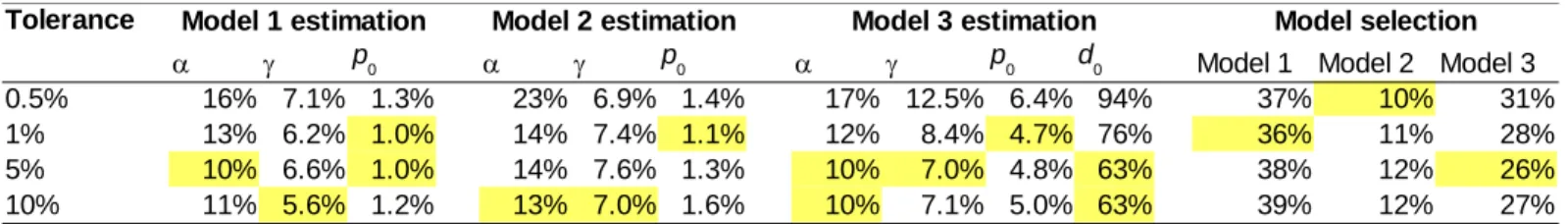
Table S1: Relative estimation and model selection errors calculated by cross-validation, as a function of the tolerance level (% of accepted simulations). The lowest value for each estimate is highlighted. For parameter estimation, the relative error is the mean square difference between the true parameter value and the estimated value, divided by the variance of the true parameter value across the 100 cross-validation replicates. The model selection error for model i is the fraction of cross-cross-validation replicates of model i where the selected model was not i.

Tolerance Model 1 estimation Model 2 estimation Model 3 estimation Model selection

a g a g a g Model 1 Model 2 Model 3

0.5% 16% 7.1% 1.3% 23% 6.9% 1.4% 17% 12.5% 6.4% 94% 37% 10% 31%

1% 13% 6.2% 1.0% 14% 7.4% 1.1% 12% 8.4% 4.7% 76% 36% 11% 28%

5% 10% 6.6% 1.0% 14% 7.6% 1.3% 10% 7.0% 4.8% 63% 38% 12% 26%

10% 11% 5.6% 1.2% 13% 7.0% 1.6% 10% 7.1% 5.0% 63% 39% 12% 27%

Supplementary figures

Fig. S1. Cross-validation results for the approximate Bayesian computation (ABC) estimation procedure, for (a) Model 1 (random return), (b) Model 2 (nearest return) and (c) Model 3 (distance-based return probability). For each model version, we selected a random sample of 100 (out of 10,000) simulation results, considered each one in turn as the “data” and ran the ABC-rejection algorithm (with 5% tolerance level) on the remainder of the simulation results to infer the true parameter values of the left out simulation. The diagonal line on each plot indicates equality between true and estimated values. The point estimates shown are the median of the posterior distribution, while error bars represent the 95% credible interval.

Fig. S2. Variation in the posterior parameter distribution quantiles (median and bounds of the 95% Bayesian credible interval) as a function of the number of simulations (Nsim), for (a) Model 1 (random

return), (b) Model 2 (nearest return) and (c) Model 3 (distance-based return probability). The error bars show the 95% central range for each estimate and were obtained from 100 bootstrap replicates at each value of Nsim.