Colour-Difference Assessment for Driving Headlight Simulation

Science Arts & Métiers (SAM)

is an open access repository that collects the work of Arts et Métiers Institute of

Technology researchers and makes it freely available over the web where possible.

This is an author-deposited version published in: https://sam.ensam.eu Handle ID: .http://hdl.handle.net/10985/10697

To cite this version :

Quentin VIDAL, Sylvain MICHELIN, Baptiste LABORIE, Andras KEMENY - Colour-Difference Assessment for Driving Headlight Simulation - In: Driving Simulation Conference, France, 2014-09-04 - Driving Simulation Conference - 2014

Any correspondence concerning this service should be sent to the repository Administrator : archiveouverte@ensam.eu

C

OLOUR

-D

IFFERENCE

A

SSESSMENT FOR

D

RIVING

H

EADLIGHT

S

IMULATION

Quentin Vidal1,2, Sylvain Michelin2, Baptiste Laborie4 and Andras Kemeny2,3 (1) : University of La Rochelle

Laboratoire Informatique Image et Interaction F-17042 La Rochelle Cedex 01

{quentin.vidal,sylvain.michelin}@univ-lr.fr

(2) : Technocentre Renault Technical Center for Simulation 1 avenue du Golf, F-78288 Guyancourt {quentin.vidal,andras.kemeny}@renault.com (3) : Arts et Métiers ParisTech

Laboratory of Immersive Visualization 151 Boulevard de l’Hôpital, F-75013 Paris

{andras.kemeny}@ensam.eu

(4) : OKTAL

19 Boulevard des Nations Unies F-92190 Meudon, France

{baptiste.laborie-renexter}@renault.com

Abstract – In high quality driving simulation applications, such as headlight simulation, colorimetric validity is essential. In virtual testing of headlight systems, it is important that the WYSIWYG (What You See Is What You Get) paradigm is respected for product quality headlight assessment. Indeed, if a slightly reddish orange colour is displayed instead of the typical orange of halogen lighting, the effect for driver comfort or traffic safety can be critical. The lighting specialist should accept a headlight which doesn't have the right colour.

Previous studies have shown that there is a significant colour difference between virtual and real environments. Nevertheless, in virtual headlight testing the rendered colour fidelity has to fit industrial assessment. This study therefore deals with the colour-difference perceptibility that is the ability of an observer to detect a difference between two colours and, more precisely, on the acceptability of the perceived difference.

We propose in this paper a psychophysical function for colour difference acceptability which fits well with the measured data. The colour acceptability function was implemented in a driving simulator for high validity headlight assessment. Driver acceptability experimentation was carried out using Renault's headlight driving simulation equipped with a full-cab and a 210° cylindrical display screen.

Key words: Colour-Difference Acceptability, Virtual Reality, Psychophysical Threshold.

1. Introduction

Virtual environments are gaining widespread acceptance as a tool for assessing the quality of physical prototype such as vehicle headlights. In a context of high quality simulation applications, it is essential that a displayed colour is as near as possible to the real one. Indeed, if a slightly reddish orange colour is displayed instead of the typical orange of halogen lighting, the effect for driver comfort or traffic safety can be critical. The lighting specialists should accept a headlight which doesn't have the right colour.

Previous internal investigation has shown that a significant colour difference exists between virtual and real environments. In a critical application such as the evaluation of vehicle headlights, the acceptability of that difference as to be evaluated.

1.2. Related works 1.2.1. Colour perception

For the human colour perception, the CIE (Commission Internationale de l'Eclairage) has defined two widely used colour spaces: CIELAB and CIELUV [CIE1]. Both spaces are derived from the CIE XYZ colour space and are known to be pseudo-uniform which mean that the perceived difference between two colours depends on their locations in that space. Because of this non-uniformity, the computation of the perceived difference in the CIELAB space has evolved. The first metric , released in 1976, is define as the

Euclidean distance. This formulae has been succeeded by three other reputed metrics: , [CIE1] and [Sha1]. Those new metrics introduce application-specific weights which are unknown for our application. That's why, when the notion of difference appears in this article it refers to the first metric. Using the , it is often considerate that the JND (Just Noticeable Difference) is 1 unit which means that no difference can be seen between two colours if the difference between them is under that value [Kan1] [Mah1]. Later, using the

,

Due to the variety of observers, the difference acceptability is harder to define. Abrardo et al. [Abr1] evaluated the VASARI scanner and classified a difference between 1-3 as “very good quality", 3-6 as “good quality", 6-10 as “sufficient” and over 10 as “insufficient". Hardeberg [Har1] defines a rule of the thumb where the difference is “acceptable" if it's between 3 and 6. Lastly, Thomas [Tho1] extended Hardeberg's rule by taking into account the difference between an expert and a consumer.

1.2.2. Psychophysical methods

For the determination of a correlation between a physical stimulus (objective) and the perception of it (subjective) a psychophysical task have to be made. In this psychophysical experiment where a series of colours tests are compared with a reference, a threshold can be computed from the statistical count of accepted and non-accepted colour differences [Lab1].

Among the existing methods, Ehrenstein et al. [Ehr1] made a classification of those which have proven to be most useful in that research field: method of adjustment, method of limits, method of constant stimuli, adaptive testing, forced-choice methods.

Four of the five previous methods can only be used for the determination of a threshold between two categories and cannot be adapted for the determination of an acceptability rate which is dependant of the consumer's will. In this kind of context, the method of the constant stimuli had to be selected [Wic1].

Furthermore, for the evaluation of the colour acceptability another aspect have to be taken into account. Indeed, when asked to provide a visual judgment, an observer may interpret the

acceptable colour-difference, depending upon the intended or anticipated end use of the product. Thus colour-difference acceptability results from a compromise between the process outcome and the customer expectations [Lab1].

2. Experiments

In this section, we describe two different experiments that were conducted with two objectives: (1) allowed us to compute a psychological function which relates the percentage of acceptability in function of a colour difference to a reference, and (2) compute a threshold between acceptability and unacceptability of a difference in an expert population.

The experiments took place in the lighting simulator at Renault where all the light/screen were turned off. The observer sat on the driver's sit at a distance of 3.5 meters of the screen. At that distance, with A4 patches and following the recommendation of Schanda [Sch1], the standard 10° observer was used for the colour space transformations.

For those two experiments, the observer was invited to report his degree of satisfaction on the colours similarity via a man-machine interface. He has to make his decision between four semantic categories: “Very Satisfied", “Satisfied", “Not Satisfied", “Very Unsatisfied". To understand this scale, instructions were given before the test: “Very Satisfied means that no difference can be seen and Very Unsatisfied when the difference is much too far. For the other values, imagine that you order a car or a cloth with a specific colour and you get the other one. Would you accept this difference?”.

2.1. Experiment n°1

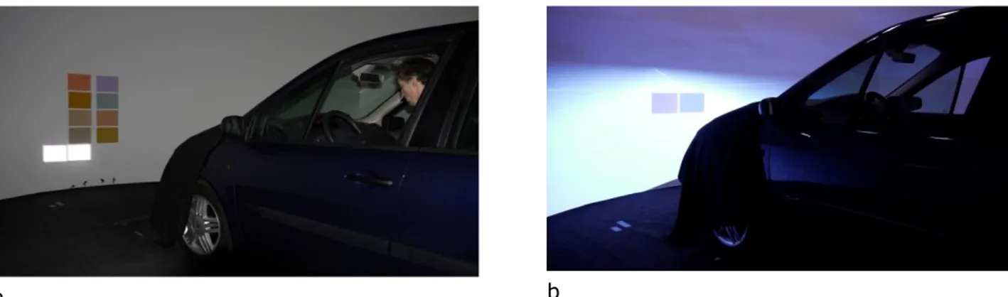
In front of the observer nine patches were disposed on the screen. During the test a computer program was responsible to randomly enlighten, via a calibrated sRGB projector Barco's Galaxy NW-12 with a gamma of 2.2 and a D65 white point, one of those patches and display a virtual colour next to it (ref. section Patch selection). Usually, for comparison of two colours a grey background is used [CIE2], for our application we used the mean colour of the rendered scene because it's in that condition that the headlights are evaluated.

a b

Fig. 1. Experimental condition for: a - experiment n°1, b – experiment n°2 To limit the experiment duration, the observer

had to take his decision about the difference in less than ten seconds. Such a time was chosen because in this time the observer can see the two patches, think if he accepts or not the difference and validate the answer. If he weren't able to make his decision during that time, the program passes to another patch.

The chosen population for this experiment was composed by 10 women and 27 men both aged 25-50. All participants had normal colour vision tested with the Ishihara’s colour deficiencies test and no one had experience with the colour management.

2.2. Experiment n°2

The aim of the second experiment is to evaluate/validate the result of the first experiment. In that purpose, the experiment was lead under the virtual environment SCANeRTM _{(i.e. the environment used by Renault}

lighting specialist). Under this environment, two patches were disposed on the road and were uniformly enlighten by the car headlights. Using the staircase method [Ehr1], the observer had to accept or not the difference between those two patches. If he accepts, the difference increase otherwise it decrease. At the beginning, the two patches were widely separated ( of 20) which force the expert to reject this first value. The initial value of the step was set to of 4 and progressively reduced to 0,125 (to compute a precise thresh the step is divided by two at each reversal).

In this experiment, the population was composed by three colour expert from Renault (design direction). Two works on the industrial quality validation and the other one on the colour & material expert assessment. Because of the expert nature of the population, it’s considered, as a predicate of this experiment, that their results should be highly closed among

themselves and the result not dependant of the number of participants.

2.3. Patch selection 2.3.1. Physical patches

The physical patches use in this experiment come from the Natural Colour System®© _and

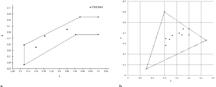
are guaranteed not to exceed 0.8. Those patches were selected because they fit the specification of the white lamps for road vehicles [AFN1] and they're in the sRGB gamut which correspond to the projector's gamut (see Fig. 2). The nine chosen patches of this evaluation are selected because: six of them correspond to the headlight gamut boundary and three to the colour coordinates of the three mains lamps used in the Renault’s headlight (LED, Halogen and Xenon).

2.3.1. Virtual patches

For the determination of the acceptability threshold, it is important to know the difference between the physical patch and the virtual one. With the value of the real patch the sRGB value can be computed following [CIE1]. However, because of the reflectivity of the screen, the colours seem different. Equalization had to be made and was validated by two colours experts (1 designer and 1 doctor in vision science).

Because of the non-uniformity of the CIELAB space, the distance from which everybody find the difference “Very Unsatisfied" have to be compute. For that point the staircase method [Wic1] have been used for the four judgements directions of each patch.

a b

Fig. 2, Patches xy coordinates in: a – headlight gamut [AFN1], b – sRGB gamut

Once the maximum distance is obtained, for each direction, the set can be divided in six equal parts. Each distance lies in

. From that distance and the value of the reference patch, the new values are computed using the CIELCH space. For each distance in chroma, the new values are computed by adding to the initial Chroma value the distance (see Eq. 1). For the difference in hue, it isn't possible to directly use the distance; it has to be converted in an angle using the law of cosine. For this, an isosceles triangle is considered (because the Chroma needs to be constant). Once the difference angle computed, the hue value is calculated by adding to the initial hue (see Eq. 2).

3. Results

3.1. Psychophysical function fitting

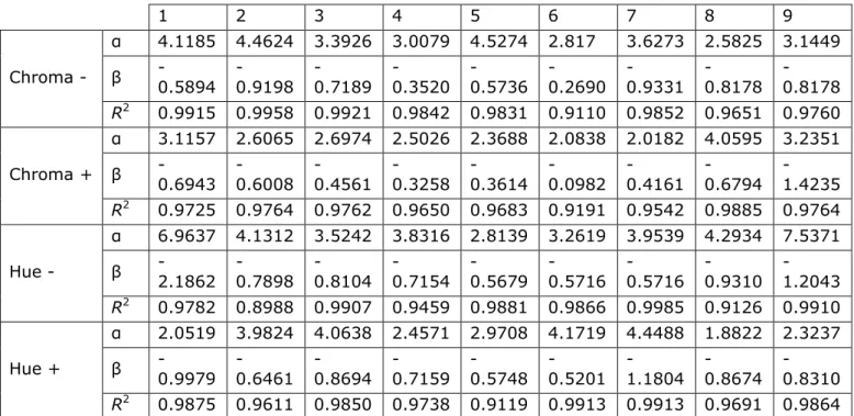
The psychophysical function is often represented by a two-parameter function F, which is typically a sigmoid function, such as the Weibull, logistic, cumulative Gaussian, or Gumbel distribution [Wic1]. This kind of shape is explained by the fact that the more a stimulus is close to a reference the more people don't see any difference and accept it. In our case, the function that best describes our distribution is the logistic one (see Fig. 3). The overall results for the function fitting is presented on Table 1 and, as expected, the parameters alpha and beta are different for each patch and for each axis. This is explained by the non-uniformity of the CIELAB-space and by the used metric.

Despite that, the function fitting is strongly correlated to the real data with only 6 of the 36 values under 0.95, a mean coefficient of determination of 0.97, a standard deviation of 0.02 and a minimum value of 0.8988.

a

Fig. 3. Sigmoid function: a – Fitting of the logistic function (green curve) with the acceptability rate data (blue dot), b – Equation of the logistic function

(1)

Table 1. Psychophysical coefficient α, β and the coefficient of determination R2 _{for each axis of each patches.} 1 2 3 4 5 6 7 8 9 Chroma - α 4.1185 4.4624 3.3926 3.0079 4.5274 2.817 3.6273 2.5825 3.1449 β -_0.5894 -_0.9198 -_0.7189 -_0.3520 -_0.5736 -_0.2690 -_0.9331 -_0.8178 -_0.8178 R2 _{0.9915 0.9958 0.9921 0.9842 0.9831 0.9110 0.9852 0.9651 0.9760} Chroma + α 3.1157 2.6065 2.6974 2.5026 2.3688 2.0838 2.0182 4.0595 3.2351 β -_0.6943 -_0.6008 -_0.4561 -_0.3258 -_0.3614 -_0.0982 -_0.4161 -_0.6794 -_1.4235 R2 _{0.9725 0.9764 0.9762 0.9650 0.9683 0.9191 0.9542 0.9885 0.9764} Hue - α 6.9637 4.1312 3.5242 3.8316 2.8139 3.2619 3.9539 4.2934 7.5371 β -_2.1862 -_0.7898 -_0.8104 -_0.7154 -_0.5679 -_0.5716 -_0.5716 -_0.9310 -_1.2043 R2 _{0.9782 0.8988 0.9907 0.9459 0.9881 0.9866 0.9985 0.9126 0.9910} Hue + α 2.0519 3.9824 4.0638 2.4571 2.9708 4.1719 4.4488 1.8822 2.3237 β -_0.9979 -_0.6461 -_0.8694 -_0.7159 -_0.5748 -_0.5201 -_1.1804 -_0.8674 -_0.8310 R2 _{0.9875 0.9611 0.9850 0.9738 0.9119 0.9913 0.9913 0.9691 0.9864}

Even if the data were highly correlated to the real data some psychological function had to be remove from the set. That’s the case for the patch n°6 where its acceptability percentage doesn’t go below 25% and moves back up at the maximal difference. Because of the patch position on the sRGB gamut (see Fig 2.a) this result could have been predicted. Indeed, this patch was on the border of the gamut and the computation of the new colours using the Eq.1 and 2 generates colour that cannot be displayed by the projectors.

From that result and the knowledge that most of the time, a threshold measured with the method of constant stimuli is defined as the intensity value that elicits perceived responses on 50% of the trials [Ehr1], it’s possible to reverse the function F(x) for having the acceptable difference in function off the acceptability rate (see Eq 3.).

3.2. Expert’s validation

Like expected from an expert population, their responses for the colour difference acceptability test are closely connected with a mean standard variation of 0.49 which is under the just noticeable difference of the colour perception [Kan1]. This first result shows that the experts are agreed amongst themselves which validate our predicate for this experiment.

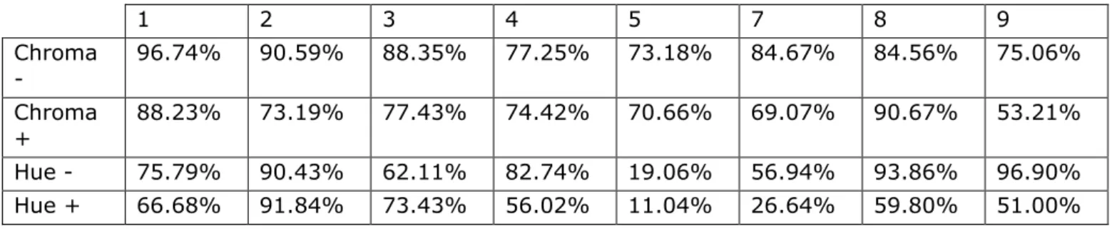
From the computed expert acceptation threshold and the function giving the percentage of colour-difference acceptability in the normal population, it’s possible to know how are situated the expert population compared to the normal one (see Table 2). This data set shows that Renault’s colour experts do not accept a colour difference when 71.3% of the normal population accepts it. However, it seems that some values of the set are significantly different of the others (like the patch n°5 with the negative hue).

For cutting-off highly influential values, it is supposed that the acceptable difference for the expert population match a particular percentage in the normal one. In such a case, we can model the problem by a linear regression with a null slope and a y-intercept equal to the mean of the set.

The outlier suppression is performed using the Cook’s distance which measures the effect of deleting a given observation. If the distance is over the constant (with n the number of observation), a closer examination of the data have to be made [Bol1].

This test reveals that a particular attention had to be made concerning three data (bold values in Table 2). After a measure session it appears that, for those data, we were not able to reproduce the right colour . Removing those data enables us to know that the expert population does not accept a colour-difference when 76% of the normal one accepts it.

Table 2. Naïve population acceptability rates in function of the expert acceptable difference. 1 2 3 4 5 7 8 9 Chroma - 96.74% 90.59% 88.35% 77.25% 73.18% 84.67% 84.56% 75.06% Chroma + 88.23% 73.19% 77.43% 74.42% 70.66% 69.07% 90.67% 53.21% Hue - 75.79% 90.43% 62.11% 82.74% 19.06% 56.94% 93.86% 96.90% Hue + 66.68% 91.84% 73.43% 56.02% 11.04% 26.64% 59.80% 51.00%

Table 3. Colour-difference acceptability.

Expert Naïve

Mean Max Mean

Good Good Good

Acceptable Good Good

Unacceptable Acceptable Acceptable

Unacceptable Unacceptable Unacceptable

4. Discussion

The first experiment shows that the computed s-shaped curves are strongly correlated to the data with a mean coefficient of determination of 0.97. Like we expected, because of the non-uniformity of the CIELAB-space the coefficients of each curve are different. Another interesting thing which will not be discussed here is that instead of separating the hue/chroma into a negative and a positive, it was also possible to take the whole hue/chroma data and fits a Gaussian curve.

The second experiment indicates that for a high quality application such as the headlight assessment, the common 50:50% threshold [Ehr1] isn’t optimal. Indeed, colour expert from Renault find unacceptable a colour difference when 76% of the normal one accepts it. With this value and the equation 3, the corresponding value of the colour-difference is computed and the following table constructed.

The values 3.1 and 4.8 are respectively computed using the 76% and 50% of acceptability rates. For the expert population, in addition to the mean difference, the maximum difference is added. Indeed, the global scene can have a good representativity but cannot display correctly the road line marking colour which is used by the headlight expert for assessing the headlight quality.

5. Conclusion

In this paper, we present a method for assessing the acceptability of a colour-difference of a

driving car simulator. In that purpose, we have lead two psychological experiments; the first one with naïve people and the second one with colour expert from Renault. Those experiments enable us to construct a colour-difference acceptability scale which directly reflects the perception of the observers (expert and non-expert).

Besides, we found that a significant difference exist between the naïve and the expert population, this result is in agreement with a previous study lead by Shamey et al. [Sha2] where they found a significant difference between the two populations in the assessment of small colour differences. This difference, can be explained by the fact that expert are accustomed to this task and have an a priori knowledge on what they accept or not [Mil1]. A limit to our method is the use of the old metric , a future work would be to determine the best colour-difference metric for a driving car simulator. Another improvement point would be the use of more colours in the experiment. Indeed, nine colours are enough for the evaluation of the headlight rendering but in a more complex scene there are more colours which lead us to the evaluation of more colours.

Another interesting point that wasn’t discuss here is that our data can also be approximated by a Gaussian curve which isn’t centred on . This means that the observer finds a colour slightly different better than the same colour.

6. References

[Abr1] Abrardo A., Cappellini V., Cappellini M. and Mecocci A., “Art-works colour calibration using the VASARI scanner.”, Color Imaging Conference, IS&T - The Society for Imaging Science and Technology, 1996, pp. 94-97.

[AFN1] Association Française de Normalisation, “Lamps for road vehicles - Dimensional, electrical and luminous requirements”, AFNOR pub., NF EN 60809/A4, 2009.

[Bol1] K. A. Bollen and R. W. Jackman “Regression Diagnostics An Expository Treatment of Outliers and Influential Cases”, Sociological Methods & Research, 1989, 13(4), pp 510-542.

[CIE1] International Commission on Illumination, “Technical Report – Colorimetry”, Pub. 15:2004 3rd ed, ISBN 3-901906-33-9, 2004.

[CIE2] International Commission on Illumination, “Parametric effects in colour-difference evaluation”, Pub. CIE 101-1993, ISBN 978 3 900734 38 1, 1993.

[Ehr1] Ehrenstein W. H. and Ehrenstein A., “Psychophysical Method”, Modern Techniques in Neuroscience Research, Chap. 43, 1999.

[Gib1] Gibson J. E., Fairchild M. D., “Colorimetric characterization of three computer displays (LCD and CRT)”, Munsell Color Science Laboratory Technical Report, 2000.

[Har1] Hardeberg J. Y., “Acquisition and reproduction of colour images: colorimetric and multi-spectral approaches”, Master Thesis at Ecole Nationale Supérieure des Télécommunications, 1999.

[Kan1] Kang. H. R., “Color Technology for Electronic Imaging Devices”, SPIE Optical Engineering Press., 1994.

[Kem1] Kemeny A., Combe E. and Posselt J., “Perception of Size in Vehicle Architecture Studies”, Proceedings of the 5th _Intuition

International Conference, 2008.

[Lab1] Laborie B., Viénot F., Langlois S., “Methodology for constructing a colour-difference acceptability scale”, Journal of Ophthalmic and Physiological Optics, 2010, 30(5).

[Loo1] Loomis J. M. and Knapp J. M., “Visual perception of egocentric distance in real and virtual environment”, Virtual and Adaptive Environments, 2003, pp. 21-46.

[Mah1] Mahy M., van Eycken L. and Oosterlinck A., “Evaluation of uniform color spaces developed after the adoption of CIELAB and

CIELUV”, Color Research and Application, 1994, 19(2), pp. 105-121.

[Mil1] Miller A.M., “The Magical Number Seven, Plus or Minus Two: Some Limits on Our Capacity for Processing Information”, The Psychological Review, 1956, vol. 63, pp. 81-97. [Tho1] Thomas J. B., “Colorimetric characterization of displays and multi-display systems”, Master Thesis at University of Bourgogne, 2009.

[Sch1] Schanda J., “Colorimetry: Understanding the CIE system”, John Wiley & Sons, ISBN 9780470175620, 2007.

[Sha1] Sharma G., Wu W. and Dalal E. N., “The CIEDE2000 Color-Difference Formula: Implementation Notes, Supplementary Test Data, and Mathematical Observations”, Color Research & Applications, 2004, 30(1), pp. 21– 30.

[Sha2] Shamey R., Cardenas L. M., Hinks D. and Woodard R., “Comparison of naïve and expert subjects in the assessment of small color differences”, Journal of the Optical Society of America, 2010, 27(6), pp. 1482-1489.

[Wic1] Wichmann F. A. and Hill N. J., “The psychometric function: I. Fitting, sampling, and goodness of fit”, Perception & Psychophysics, 2001, 63, pp. 1293-1313.