Science Arts & Métiers (SAM)
is an open access repository that collects the work of Arts et Métiers Institute of
Technology researchers and makes it freely available over the web where possible.
This is an author-deposited version published in: https://sam.ensam.eu Handle ID: .http://hdl.handle.net/10985/8641
To cite this version :
Florent MARGNAT, Xavier GLOERFELT - On compressibility assumptions in aeroacoustic integrals: a numerical study with subsonic mixing layers - The Journal of the Acoustical Society of America - Vol. 135, n°6, p.3252 - 2014
On compressibility assumptions in aeroacoustic integrals:
a numerical study within subsonic mixing layers
Florent Margnata)
Institute PPRIME, Department of Fluid Flow, Heat Trans-fer and Combustion, Universit´e de Poitiers - ENSMA - CNRS Building B17 - 6 rue Marcel Dor´e - TSA 41105
86073 POITIERS CEDEX 9 - France Xavier Gloerfelt
Arts et Metiers ParisTech, DynFluid Lab, 151 boulevard de l’Hopital, 75013 PARIS, France
(Dated: March 24, 2014)
Two assumptions commonly made in predictions based on Lighthill’s formalism are investigated: a constant density in the quadrupole expression, and the evaluation of the source quantity from incompressible simulations. Numerical predictions of the acoustic field are conducted in the case of a subsonic spatially evolving two-dimensional mixing layer at Re = 400. Published results of the direct noise computation (DNC) of the flow are use as reference and input for hybrid approaches before the assumptions on density are progressively introduced. Divergence free velocity fields are obtained from an incompressible simulation of the same flow case, exhibiting the same hydrodynamic field as the DNC. Fair comparisons of the hybrid predictions with the reference acoustic field valid both assumptions in the source region for the tested values of the Mach number. However, in the observer region, the inclusion of flow effects in the Lighthill source term is not preserved, which is illustrated through a comparison with the Kirchhoff wave-extrapolation formalism, and with the use of a convected Green function in the integration process.
PACS numbers: 43.28.Ra, 43.20.Wd
I. INTRODUCTION
The overall problem area addressed here is that of es-timating the noise radiated by unsteady flows. We aim at improving the class of methods in two steps, usually described as hybrid, which use experimentally or numeri-cally generated flow data as an input for solutions of wave propagation equations, in particular those solutions writ-ten with an integral formalism such as Lighthill’s analogy and the Kirchhoff wave extrapolation method. Because the two-step approach allows cost reduction in the es-timation of the radiated field, hybrid methods are fre-quently chosen for the prediction of flow generated noise in many applications such as jet, high-lift devices and landing-gear on planes, car mirror and window vortex, fans, propellers, etc. That prediction consists in extract-ing among the unsteady motions in the flow those able to excite outward propagating sound waves. Consequently, once it is obtained, the analysis of the acoustic field and its correlation to the flow events can be conducted in or-der to identify the noisy vortical motion. In that sense, hybrid methods may also help the physical understand-ing of aeroacoustic issues.
Any analogy approach relies on the explicit knowl-edge of the source quantity that excites the wave opera-tor. Since Lighthill’s initial derivation1 of an inhomoge-neous wave equation from the equations of motion, with a source term defined by the flow quantities, a constant
a)Electronic address: [email protected]
research effort has been devoted to improve its potential, from theoretical works on the source term and surround-ing flow effect modellsurround-ing, to numerical works increassurround-ing quickness and accuracy of the solution. In particular, Crow2 investigated analytically the distinct role of the compressibility in the source term and in the wave oper-ator. By the method of matched asymptotic expansion, he concluded that, for low Mach number and compact source region, Lighthill’s solution for the density is ade-quate if the latter is assumed constant in the quadrupole. Because Lighthill’s equation is an exact rearrangement of the flow equations, it contains flow effects on acoustics such as wave convection and refraction. The left-hand side being the wave operator without flow, those effects are included in the source side. Consequently,the source term thus obtained is not the true3 acoustic source, be-cause it accounts for other phenomena in addition to acoustic energy production. Questing for such a reduced source expression, Lilley4and Ribner5derived an analogy equation for jet noise modelling, through the specification of unidirectional, transversely sheared, mean flow in the Lighthill source term, so that its solution displays sound refraction by velocity gradients. This was numerically applied to a mixing layer by Colonius et al6. Recently, Suzuki & Lele7 derived approximate Green functions for a source in a mixing layer. It should be the appropriate propagator to associate, in the convolution integral, with a source expression that would be purified from convec-tion and refracconvec-tion effects.
The full knowledge of the source term with fine space and time resolutions brought by the numerical simulations allows to check the validity of assumptions
made in theoretical or experimental studies. Moreover, building reduced-order models of the flow may reduce the computational cost of closed-loop control systems. In that context, Samanta et al8 studied the sensitivity of several analogy formulations to errors intentionnally introduced into the source quantity, namely removing the highest modes from the decomposition or perturbat-ing the most energetic ones.
The present contribution builds on these efforts to characterise the content of the Lighthill source term, in order to provide background for current source term eval-uation in analogies. The assumptions regarding density are investigated numerically, through the association of a constant density with compressible velocity fields, as well as the evaluation of the quadrupoles from fully incom-pressible data. We also analyse how those assumptions are sensitive to Mach number variations and how they af-fect the inclusion of flow effects on acoustics in Lighthill’s formalism. For the latter, the convected wave equation and the Kirchhoff formalism are used as reference points. Numerical evaluations of aeroacoustic integrals are thus conducted in the frequency domain in the case of a subsonic spatially evolving two-dimensional mixing layer at Re = 400. Such flow is free from surface effect such as reflexion or diffraction, thus focusing our analysis on the original source term. Moreover, a two-dimensional con-figuration allows the integration of many source quanti-ties over many volume extents with an affordable compu-tational effort. The integrands are read from databases generated by the numerical solution of the Navier-Stokes equations. A direct noise computation (DNC) provides the compressible velocity, pressure and density fields, and the reference result for the acoustic field at the same time. In addition, an incompressible simulation provides the source quantity using divergence free velocity field. To the best of the authors’ knowledge, the resolution of Lighthill’s equation with source data from a DNC and an incompressible simulation of the same flow was not conducted before.
The paper is organised as follows. In section II, Lighthill’s and Kirchhoff’s formalisms are recalled in the Fourier space, for either a convected wave equation or a propagation in a medium at rest. In section III, the mixing-layer parameters are presented along with the nu-merical methods applied for the flow simulations and in-tegral evaluations. The coherence between the several prediction strategies is checked in section IV, and the inclusion of the convection effect in the Lighthill source term is illustrated. The influence of compressibility in the evaluation of the quadrupoles is then adressed in sec-tion V. Eventually, the main results of the paper are summarised and further discussed in section VI.
II. MATHEMATICAL FORMULATION A. Kirchhoff’s formalism
For a moving medium, the acoustic pressure p′ at any time t and location x in a volume V is related to the
distribution Q of sources within V and the distribution of the pressure and its derivative on the boundary of
V , noted Σ, by the generalised Green formula9. For a 2-D configuration, with U∞ = (U∞, 0) in the observer
domain, it can be written as
p′(x, t) = ∫ ∞
−∞ ∫∫
V
Q(y, τ ) ˜G(x, t|y, τ)dydτ
+ ∫ ∞ −∞ ∫ Σ { ˜ G∂p ′ ∂yi − p′∂ ˜G ∂yi } nidΣ(y)dτ +U ∞ c2 0 ∫ ∞ −∞ ∫ Σ { p′D∞ ˜ G Dτ − ˜G D∞p′ Dτ } n1dΣ(y)dτ (1)
where n = (n1, n2) is the unit normal vector pointing inward the observer domain V , c0 is the sound speed of the ambient fluid, D∞/Dt = ∂/∂t + Ui∞∂/∂xi, and ˜G is the time-domain Green function solution to the uni-formly moving medium wave equation. By taking the following Fourier transform:
F [f (x, t)] = f (x, ω) =
∫ ∞ −∞
f (x, t)e−iωtdt (2)
where ω is the angular frequency and i2 =−1, formula (1) reduces to the form
p′(x, ω) = ∫∫
V
Q(y, ω)G(x|y, ω)dy
+ ∫ Σ { G(x|y, ω)∂p ′(y, ω) ∂yi −p′(y, ω)∂G(x|y, ω) ∂yi } (ni− M∞2n1)dΣ(y) +2iωM∞ c0 ∫ Σ
p′(y, ω)G(x|y, ω)dΣ(y) (3) where the time factor exp(−iωt) has been omitted. The Green function for the propagation in a uniform flow is given in the 2-D frequency domain by10–12:
Gc(x|y, ω) = i 4βexp ( iM∞kr1 β2 ) H0(2) ( krβ β2 ) (4) where y = (y1, y2) and x = (x1, x2) are the source and observer locations respectively, and ri = xi − yi.
Hν(m) is the Hankel function of order ν and kind m,
k = ω/c0, β2 = 1− M∞2 is the Prandtl-Glauert fac-tor, and rβ =
√
(x1− y1)2+ β2(x2− y2)2. The Green function for the uniform medium at rest, and the related pressure formula, are recovered when M∞ is set to 0.
In our configuration sketched in figure 1, the extrap-olation of the acoustic waves from the control surface Σ = (y2= ys2)∪ (y2=−y2s) is obtained by the following formula: p′(x, ω) = n2i 4β ∫ Σ [ ∂p′ ∂y2 H0(2) ( krβ β2 ) −p′krβ β2 H (2) 1 ( krβ β2 )] exp ( iM∞kr1 β2 ) dy1 (5)
Kirchhoff integral (5) theoretically predicts the acoustic pressure field provided that no source phenomenon is left
FIG. 1. Configuration and notations for the application of aeroacoustic integrals to the mixing layer flow.
inside V , that the pressure distribution on Σ contains the acoustic information generated by the sources outside V , and convection is the only flow effect acting inside V .
B. Lighthill’s formalism
Lighthill’s equation combines the mass and momentum conservation equation to form an inhomogeneous wave equation for the density. Consequently, for an observer located in the acoustic (isentropic) region, the solution for the 2-D acoustic pressure field is given, in the fre-quency domain, by:
p′(x, ω) = i 4
∫∫ D
S(y, ω)H0(2)(kr) dy (6)
where D is the source region and r = ||x − y||, for a propagation in an unbounded medium at rest. In (6), S is the Lighthill source term, defined by:
S = −∂ 2T ij ∂yi∂yj = −∂ 2 ∂yi∂yj [ ρuiuj+ (p′− c20ρ′)δij+ τij ] (7) where ui are the components of the velocity field u = (u, v), ρ′ is the density fluctuation from its value in the medium at rest and τij stands for the components of the viscous stress tensor τ .
Expression (6) can be transformed taking the space derivatives over the Green function instead of the source term, leading to:
p′(x, ω) = −i 4 ∫∫ D [ k2rirj r2 H (2) 2 (kr) −kδij r H (2) 1 (kr) ] Tij(y, ω) dy (8)
In the case of a propagation in a uniform flow at U∞= (U1∞, U2∞), the derivation of a convected wave equation11 yields: p′(x, ω) = ∫∫ D Sc(y, ω)Gc(x|y, ω) dy (9) where Sc= ∂2Tc ij ∂yi∂yj (10) =∂ 2[ρ(u i− Ui∞)(uj− Uj∞) + (p′− c20ρ′)δij+ τij ] ∂yi∂yj
Note that it is not harmless for the physical interpreta-tion that the source expression depends on the propaga-tion medium governing equapropaga-tion. It is indeed an intrinsic consequence of the analogy formalism, as explained by several authors3,8,13.
Similarly to the non-convected case, the space deriva-tives can be analytically transferred to the Green func-tion instead of numerically estimated on the source term. The second-order derivatives of the convected Green function (4) are given in11.
III. FLOW CONFIGURATION AND NUMERICAL TOOLS A. Reference flow and source data
As a reference, the acoustic field radiated by a spatially evolving subsonic mixing layer is obtained by directly solving the compressible Navier-Stokes equations on a spatial domain containing both the mixing region and the acoustic far field. The flow configuration and solver are the same as in ref.14.
The frame origin is at the inflow on the centerline, and the mean inflow velocity profile, illustrated in figure 1, has a hyperbolic tangent shape
¯ u(0, y2) = Uc+ ∆U 2 tanh ( 2y2 δω ) (11)
where Uc =U1+U2 2 and ∆U = U1− U2, noting U1and U2 the high- and low-speed flow respectively. The vorticity thickness, which varies in the streamwise direction, is defined as δω(y1) = ∆U max y2 ( ∂ ¯u ∂y2 ) (12)
Its value at the inflow is noted δω and is taken as the reference length throughout the paper.
Two subsonic isothermal cases with U1 = 2U2 are considered here, with different value of M = ∆U/c0: 0.25 and 0.40. The Reynolds number is defined by
Re = ρ0δω∆U/µ, where ρ0 is the density of the sur-rounding fluid (set to unity in those adimensionalized equations) and µ is the dynamic viscosity, and its value is fixed at Re = 400. In order to obtain a periodic and spatially fixed vortex pairing phenomenon, the flow is pertubed just downstream of the inlet, at the frequency
f0 = 0.132Uc/(δω,f) (where δω,f = 2δω is the local
vor-ticity thickness at x ≈ 80), and its first subharmonic
f0/2, using a divergence-free forcing function with low amplitude, as presented in ref.14.
The space derivatives are evaluated using sixth-order compact finite difference schemes, while a third-order
Runge-Kutta scheme provides the time marching. Fi-nally, the boundary conditions are written using a char-acteristic formulation, and terms are set inflow and out-flow. The computational domain lays over 800δωin both directions. The grid size is (2071× 785). It is stretched from the centerline in y2 direction. In y1 direction, it is almost constant below 400δω, and streched after, com-bined with a dissipation function to create the sponge zone. The flow solver and numerical parameters are de-scribed in details in ref.14.
These simulations provide both the reference acoustic field and the input data for the Kirchhoff solution (5) and the computation of the Lighthill source quantities (7), (10), (15) and (16).
B. Hybrid method implementations
Thanks to the periodic nature of the flow, the com-putation of the aeroacoustic integrals can be conducted in the frequency domain thus avoiding the integration over the whole history of the time series that is implied by 2D Green function in the time domain . Standard Fast Fourrier Transform routines are applied to the source time series. The latter are recorded about 500 times a period from the direct computation. The Hankel functions are computed using Amos library15. A mid-panel quadrature is implemented for the integra-tion of the Lighthill source term, while the Kirchhoff surface integral are evaluated with a trapezoidal rule. Streamwise, the integration domain extends over the whole DNC domain. The observer grid covers the DNC domain and is uniform with 150 points in each direction, leading to ∆xf0/c0 ≈ 8. For the formulations based on a convected wave equation, one sets U∞ = (U1, 0) and
M∞= U1/c0 for the high-speed flow, and U∞= (U2, 0) and M∞= U2/c0 for the low-speed flow.
The truncation of the source domain, typically at the outflow, can be treated either by a dissipation region, a spatial weighting, or the addition of a residual term based on the Reynolds transport theorem16 accounting for the missed region. Here, the two first techniques are used. Indeed, the dissipation function used in the direct com-putation prevents the paired vortices to generate spurious acoustic waves as they pass outflow, but their damping is not sufficient to avoid a strong contribution to the in-tegral. Thusa weighting function based on a Tukey win-dowing is applied to the source term (7). With respect to the spatial top-hat window which is de facto applied when integrating (6) over the computational domain, such weighting function reduces the spectral leakage17, that is spatial spurious noise directly translated into tem-poral noise through the dispersion relation. The source term expression in the convected form (10) appeared more sensitive to truncation effects, that is why a weight-ing of the followweight-ing Gaussian form is applied:
W (y1) = exp ( − [ y1− y10 σ(yL 1 − y10) ]4) (13) where y0
1 is the position before which W is set to 1., yL1 and σ being adjusted by the user for a given computa-tional configuration in order that no radiation is emit-ted from the outflow. Those weighting functions have a streamwise extent from 500δωto the outflow boundary.
The numerical singularity in the Hankel function, ap-pearing when the observer is located inside the integra-tion domain, can be treated by removing a small disk around it when computing the integral18, or by setting the observer grid in a staggered way with respect to the source grid. That latter solution suits better when the spatial derivatives are evaluated on the Green function itself.
IV. COHERENCE OF THE PREDICTION STRATEGIES A. Validation of the hybrid methods
The present bi-harmonically excited mixing layer ex-periences a periodic vortex-pairing phenomenon, which occurs around y1 = 200δω, and which generates acous-tic waves at that pairing frequency. The resulting instantaneous acoustic pressure field, obtained by the DNC, is plotted in figure 2a). Both Kirchhoff’s (5) and Lighthill’s (9) formalisms, based on a convected Green’s function and fed by source data from the DNC, accu-rately predict that acoustic field, as visible in figure 2b) and 2c). The comparison is fair with the field directly computed solving the compressible Navier-Stokes equa-tions plotted in figure 2a). In particular, the wavefront pattern, with a maximum radiation around θ = 50o on both layer sides, is well recovered (here and henceforth,
θ is the angle counted counterclockwise from the
down-stream direction and centered on the pairing location). In figure 2d), the acoustic field is plotted resulting from the numerical evaluation of Lighthill’s solution (6) with the Green function for an observer medium at rest inte-grated over the full DNC domain. The fair comparaison to the field directly computed illustrates well that the Lighthill analogy accounts for the convection effects, yet this is the case here because the source data come from the DNC itself and the integration domain extends over the whole observer region. The integration of a source term estimated from a compressible solver, over a do-main including the observer, is then found equivalent to the application of a convected Green function to a lo-calised source region, as firstly described by Goldstein9 and numerically illustrated by Bogey et al19. As shown in section V, that does not hold any more when a con-stant density is assumed in the quadrupole.
The mean square value of the fluctuating pressure is plotted in figure 3a) on a circle at r = 150δω away from the apparent source location (x1= 200δω, x2= 0). This quantity approaches the acoustic intensity in the far field, and provides here a more quantitative comparison be-tween the four methods. They agree well for all radi-ation angles. In particular, the level fall for increasing
|θ| is perfectly reproduced by the hybrid methods. For |θ| higher than 90o, some directivity lobes are visible, at very low levels. The method using the integration of the
FIG. 2. Instantaneous acoustic pressure field of the mixing layer, predicted by a) DNC b) Lighthill’s analogy with convected Green’s function (9), c) the convected Kirchhoff method, and d) Lighthill’s analogy (6) with the full source domain. Levels are the same for each field, linearly increasing from−4.0 × 10⁻⁵c20 (black) to 4.0× 10⁻⁵c20 (white).
−150 −100 −50 0 50 100 150 10−11 10−10 10−9 θ (deg.) < p,2 > a) DNC Lighthill ∫ S*G Lighthill ∫ S c*Gc Kirchhoff 20 40 60 80 0 50 100 150 200 250 b) y 2 s / δω E1 Lighthill ∫ S c*Gc Kirchhoff 10 20 30 40 50 0.0 0.2 0.4 0.6 0.8 1.0
FIG. 3. a) Acoustic intensity at r = 150δω predicted using 4 approaches. b) Influence of the source domain extent and control
surface location.
source term over the whole domain is the most affected by this artefact, especially on the low-speed side.
In figures 2 and 3a), the control surface used in the Kirchhoff method is defined by y2s = 40δω, whereas the convectedLighthill source term is integratedover the vol-ume inside this surface. How the predicted acoustic field depends on the control surface position and on the source extent is analysed through figure 3b), where the error with respect to the DNC is plotted, being defined as:
E1=||I
Hybrid(x)− IDN C(x)||
||IDN C(x)||
(14) where I is the acoustic intensity and||f(x)|| is the mean value of|f| over a set of observer points. Here, that set is defined as the line x2= 300δω for 100≤ x1/δω≤ 500. For both hybrid methods, the error converges towards a constant value of about 5% for ys
FIG. 4. Hybrid computations with the non-convected Green function. a) Lighthill’s analogy (6) integrated over DSOU RCE: |y2/δω| < 40; b) Kirchhoff’s method (5) with M∞ = 0 for ys2 = 40δω; c) Lighthill’s analogy (6) integrated over DOBS:
40 <|y2/δω| < 400; and d) sum of b) and c). The sum of a) and c) is identical as figure 2d). Levels are the same for each field,
linearly increasing from−4.0 × 10⁻⁵c2
0 (black) to 4.0× 10⁻⁵c20(white).
behavior is different for lower values. The convected Lighthill computation reaches the steady error level from
ys
2 ≈ 10δω after a regular decrease from unity. For the Kirchhoff computation part, the error is much higher when the control surface is located very close to the layer, and it catches the Lighthill curve only for y2s& 30δω.
From this result, the conclusion is that the acoustic source mechanism is confined in |y2| ≤ 10δω, and that below y2 ≈ 30δω, the fluctuations associated with the vortex dynamics dominate in the pressure field and pre-vent the Kirchhoff integral from a correct extrapolation of the acoustic waves.
B. Uniform flow effect
A decomposition of the integration domain D is now introduced, in order to analyse convection effect inclusion in the Lighthill source term from a spatial point of view. Using the notations presented in figure 1, the region de-fined by|y2| < y2Sis noted DSOU RCEand hereafter called ‘the source region’, while its complement with respect to
D is noted DOBSand called ‘the observation region’. Hy-brid computations are then performed using the Green function for a propagation medium at rest, that is us-ing (5) with M∞= 0 for the Kirchhoff method, and (6) with an integration over DSOU RCEfor the Lighthill anal-ogy.
The resulting instantaneous acoustic pressure fields for
ys
2 = 40δω, plotted in figure 4a) and 4b), are very sim-ilar between the two methods, but the prediction does not agree with the DNC reference shown in figure 2a). However, if the contribution of the, still not convected,
Lighthill source term with an integration over DOBS, shown in figure 4c), is added to both, the correct pattern is recovered in figure 4d) for the Kirchhoff method, and is the same as in figure 2d) for the Lighthill analogy.The lobes for|θ| ≥ 90oare again visible in figure 4d),
suggest-ing they are an effect from the acoustic/propagation do-main (ie: from the boundary conditions in the DNC), and not from the source mechanism, otherwise they should have been present in the convected Kirchhoff prediction in figure 2c).
The convection effect can thus be provided to the wave extrapolation from a Kirchhoff surface by the integration of the Lighthill source term over the observer domain, which plays here exactly the same role as the convected Green function, that is, schematically:
∫ |y2|=ys2 { Gc ∂p′ ∂n − p ′∂Gc ∂n } dy1≈ ∫ |y2|=y2s { G∂p ′ ∂n − p ′∂G ∂n } dy1+ ∫∫ |y2|>ys2 S· G dy
Note that the Kirchhoff formalism leads to the same flow quantity in the integrand, namely the pressure and its normal derivative to the control surface, for both the convected and static medium wave equations, unlike the Lighthill formalism, for which the source term expres-sion is dependent on the specific choice of the propa-gation operator3. The fully compressible solution was needed for that illustration, which may not improve the efficiency of hybrid methods,though it confirms the ro-bustness of the interpretation of Lighthill’s equation as an implicit equation for (aero)acoustic propagation within a uniformly moving flow. Moreoverit is of theoretical
in-terest that, within the integration process, the convected action of the Ligthill source term is spatially limited to the observer region (provided that the Kirchhoff surface accounts for the whole source process).
Now that the hybrid approaches have been validated when the source quantity is evaluated from the DNC, whether the density variations should be included in the Lighthill source term to ensure a correct prediction is investigated in the following.
V. DENSITY VARIATIONS IN THE QUADRUPOLES
Attempting to separate a purely radiating part from flow induced effects, Cabana et al.13suggested a decom-position of the Lighthill source term, featuring density gradient, dilatation and vorticity from the double diver-gence. Subterms including the two formers were iden-tified as a compressible reaction to subterms ideniden-tified as driving terms based on vorticity and kinetic energy. Margnat & Fortun´e20 applied that decomposition to the spatially evolving mixing-layer and noticed the impor-tance of the dilatation transport term to account for the mean flow effect. Moreover, applying the Reynolds de-composition to density and velocity components of the Lighthill tensor, Moser et al.14 reported a significant ef-fect of the term made up with density fluctuations and mean streamwise velocity when the Mach number is in-creased. Those studies pose the question of the preserva-tion of the source and propagapreserva-tion mechanisms included in the Lighthill source term when the density field is sub-mitted to assumptions,as it may occurin both theoreti-cal works and hybrid predictions.
A. Two assumptions about compressibility
The analogy approach assumes that the flow drives the acoustics with no feedback from the latter, so that Lighthill’s equation can be solved explicitely once the source distribution is known. This is theoretically valid for weakly compressible flows, say, low Mach numbers. In the absence of heating, once a low Mach number is assumed, it is tempting to assume a constant density in the evaluation of the source term, thus replacing ρ by ρ0 in the source expression, that is:
S ≈ ρ0 ∂2 uiuj ∂yi ∂yj = S0 (15) Similarly, we define Sc,0= ρ0 ∂2 ∂yi∂yj [ (ui− Ui∞)(uj− Uj∞) ] (16) This assumption is usually made when the source quantity is evaluated from experimental data in flows without significant density variations (subsonic and isothermal flows): the compressible content of the ve-locity field is preserved, while density gradients are ne-glected. It is also often assumed in theoretical works, e. g.21.
FIG. 5. Hybrid predictions based on Lighthill’s analogy with a constant density in source subterms. The acoustic pressure field radiated by a) Sc,0with the convected Green function; b) S0integrated over the full DNC domain. Levels are the same
for each field, linearly increasing from−4.0 × 10⁻⁵c20 (black)
to 4.0× 10⁻⁵c20 (white). DSOU RCE and DOBS are defined as
inside and outside|ys
2| = 40δωrespectively.
For the present mixing layer, figure 5a) shows that neglecting density variations does not alter the acous-tic prediction using Lighthill’s analogy in the convected form (10). However, for the form (7) that includes the convection effect in the source term, it does, as visible in figure 5b),yielding an incorrect wave pattern.
Note that in acoustic motions, the fluctuating activity involves the pressure and the velocity together with the density, meaning that a constant density assumption will not remove the acoustic part of the Lighthill source term contained in the velocity field. An incompressible simu-lation, however, will lead to a source quantity evaluated with a divergence-free velocity field, that is:
Sc≈ ρ0 ∂2 ∂yi∂yj [ (ˆui− Ui∞)(ˆuj− Uj∞) ] = ˆSc,0 (17)
where ∇ · ˆu = 0. Alternately, ˆS0 = ρ0
∂2uˆ
iuˆj
∂yi∂yj . Such assumption on the source term, which is common in the use of hybrid methods, is investigated in details in the following subsections.
B. Compressible and incompressible near-fields
For the purpose of evaluating (9) under assumption (17), an incompressible simulation of the mixing layer at the same Reynolds number is conducted. The incom-pressible flow solver is that presented in22. The pertur-bation of the inflow profile (11) is only applied to the
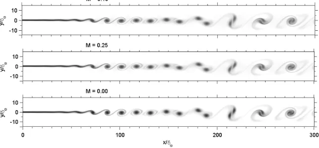
FIG. 6. Vorticity snapshots for DNC’s at M = 0.40 (top) and M = 0.25 (middle) and for the incompressible simulation (bottom). Levels are from−0.8U2/δω (black) to 0.0 (white).
transverse velocity component. The perturbation ampli-tude at f0is 0.0027U2, twice that of f0/2, while the phase between the two frequencies is 0.4π. These settings are chosen in order to obtain the same longitudinal evolution as obtained in the compressible simulations. The com-putational domain is limited to 100δωon each side of the mixing layer since the acoustic field can not be simulated. The dynamic viscosity is linearly increased on the second half of the computational domain, providing a dissipation of paired vortices before the outflow, in order to prepare the treatment of the truncation in the hybrid acoustic prediction.
The resulting vorticity field is compared in figure 6 to that from the DNC at different Mach numbers. As shown by Moser et al14 there are almost no observable differences between the vorticity field of the simulation at M = 0.25 and that of the simulation at M = 0.40. No more differences appear when the comparison includes the incompressible simulation. In the following, the ve-locity and pressure statistics in the mixing region are quantitatively compared between the incompressible sim-ulation and the two compressible cases. The Reynolds decomposition is used noting f = ¯f + f′ where ¯f is the
mean value of f over a pairing period.
The spreading of the mixing layer is characterised with the help of the streamwise evolution of a thickness. In addition to the vorticity thickness (12), two other defi-nitions are used. How far the constant velocity profiles must be moved to deliver the same mass flow leads to the displacement thickness: δ∗(y1) = ∫ 0 −∞ ( ¯ u U2 − 1 ) dy2+ ∫ +∞ 0 ( 1− ¯u U1 ) dy2 (18) Finally, the summation of the half thickness of each streamyields a third definition:
δ1/2(y1) = δ1(y1) + δ2(y1) (19)
where δ1 and δ2 are defined by ¯u (y1, δ1) = U1− ∆U/4 and ¯u (y1, δ2) = U2+ ∆U/4, respectively.
The evolutions of the three thicknesses, of the stream-wise and transverse velocity RM S fluctuations and of the instantaneous pressure fluctuation are plotted along the mixing-layer axis in figure 7. All the quantities show excellent agreement between the three simulations. In particular, the saturation of the first unstable mode oc-curs at the same position. The vortex pairing causes a global maximum of the thicknesses and the velocity tuations, and a second saturation for the pressure fluc-tuation. The fluctuations from the incompressible sim-ulation have a slower amplitude decrease at the end of the plotted domain, likely because the dissipation region is not designed in the same way. The vorticity thick-ness exhibits spurious local variations dowstream of the pairing region. Indeed, because it is defined using the maximum slope of the mean velocity profile, its compu-tation may be affected by the presence of more than one slope maximum, which happens after the pairing.
Concerning the transverse decays of fluctuations, it is shown through figure 8 that for|y2| < 25δω, the fluctu-ations of both velocity components and of the pressure, once normalized by the low-speed flow velocity, have ex-actly the same level for the three simulations. That re-gion may then be referred to as hydrodynamic. Above
|y2| = 25δω, the fluctuations from the incompressible sim-ulation go on decaying exponentially, while the acoustic fluctuations start to be dominant in the compressible sim-ulations. The latter depend on the Mach number, since they scale with M7/2 in 2D as observed in ref.14.
At this point, it is clear from figures 6, 7, and 8, that the hydrodynamic part of the flow is the same between both compressible simulations and the incompressible one. On that basis, the assumption of an incompressible velocity field can be tested in the Lighthill prediction.
100 200 300 400 0 2 4 6 8 10 δ / δω δω(y 1) δ* δ 0.5 u, v, 100 200 300 400 0.0 0.1 0.2 0.3 RMS M = 0.40 M = 0.25 M = 0.00 M = 0.40 M = 0.25 M = 0.00 0 100 200 300 400 −0.4 −0.2 0.0 0.2 y 1 / δω p, / U 2 2 Max t Min t
FIG. 7. Evolution of statistic quantities along the mixing-layer axis. Top: mixing-layer thicknesses; middle: fluctuating longitudinal and transverse velocities; bottom: instantaneous pressure fluctuation and its extreme values in time. M = 0.00 stands for the incompressible simulation.
C. Results for the convected Lighthill predictions
In figure 9, the directivity of the acoustic intensity at
r = 150δω obtained using either Sc,0 or ˆSc,0 is compared to the convected Lighthill computation using the fully compressible source term Sc. The DNC result is shown too, for reference. Three extents of the source region are considered, in order to visualise any phenomenon that could be missed where the hydrodynamic and acoustic parts coexist. A first worthnoting result appears through the intensity fall for |θ| > 50o, which is well captured by all the Lighthill predictions. Below these angles, the two sides of the mixing layer do not exhibit the same trends. On the high-speed side, the modelling of the source term does not significantly affect the prediction, even for the smallest source extent. The incompressible source term tends to yield a slight overprediction at small
|θ|, however. On the low-speed side, a strong
overpredic-tion at aft angles is observed for the three hybrid compu-tations when the source region is limited to|y2| ≤ 20δω. For larger source extents, the constant density modelling yields nearly the same result as the fully compressible source term, while the incompressible assumption still
leads to an overprediction at small|θ|, though reduced. That influence of the source extent suggests a weakly compressible phenomenon in the near-field, which affects the acoustic radiation while being accounted for by the Lighthill source term if evaluated with a compressible velocity field. Regarding this, the pressure fluctuation near-field is plotted in figure 10 for both flow simulations. The DNC makes visible a pattern of two lines of spots where the fluctuation level is strongly lower than around, like sinks, downstream after the pairing and around y2=
±30δω. The incompressible flow simulation returns only one such sink, in the vicinity of the pairing. Moreover, an asymmetry between the two streams is noticed, the high-speed flow exhibiting more similarities between the two simulations. Such near-fields may influence strongly the propagation at small angles(for which acoustic rays stay longer in the perturbed region), what could explain why any of the convected Lighthill computations miss the acoustic level there when the source domain do not include it, and why the incompressible source modelling misses this in the low-speed region even for a larger source domain.
−50 0 50 10−4 10−3 10−2 10−1 RMS y 2 / δω u, / U 2 −50 0 50 y 2 / δω v, / U 2 M = 0.40 M = 0.25 M = 0.00 −50 0 50 y 2 / δω p, / U 2 2
FIG. 8. Transverse evolution of the velocity and pressure fluctuations at x/δω= 300. M = 0.00 stands for the incompressible
simulation. −90 −45 0 45 90 10−10 10−9 10−8 a) y s = 10 δω θ (deg.) < p,2 > −90 −45 0 45 90 b) y s = 20 δω θ (deg.) −90 −45 0 45 90 c) y s = 40 δω θ (deg.)
FIG. 9. Influence of the source modelling on the acoustic directivity at r = 150δω predicted by the convected Lighthill
analogy with the fully compressible source term Sc(dashed line), a constant density assumption Sc,0 (dash-dotted line), and
incompressible velocity fields ˆSc,0 (symbols). Full line: DNC. Three extensions of the source domain, case M = 0.25.
D. Increasing the Mach number
As investigated by Moser et al14, increasing the Mach number of mixing layers with U1 = 2U2 leads to a re-inforcement of the directivity peak around θ = 50o es-pecially for the radiation towards the high-speed flow. This is illustrated in figure 11a) and figure 11c) with the instantaneous acoustic pressure field as given by the DNC for M = 0.25 and M = 0.4 respectively. That reinforcement is perfectly captured by the
incompress-ible source term modelling, as qualitatively visincompress-ible in fig-ure 11b) and figfig-ure 11d), and quantitavely confirmed by the intensity plots at r = 150δωin figure 12 showing well the intensity fall after θ ≈ 50o. In spite of the afore-mentioned flaw at aft angles, such a successful associa-tion of the incompressible source modelling with the con-vected Green function, even for the highly subsonic case at (M1= 0.8, M2= 0.4), is worth to notice.
Furthermore, it can be deduced that the effect of the Mach number on the directivity is brought by the
acous-−80 −40 0 40 80 y 2 / δω 0 100 200 300 400 −80 −40 0 40 80 y 1 / δω y 2 / δω
FIG. 10. Isocontours of the RM S pressure fluctuation in the near-field of the compressible (top) and incompressible (bottom) mixing layer, for M = 0.25. The level of a contour is twice the previous one, starting from 0.0032U22.
tic wave convection only, because the three vortical fields do not show any significant difference while the convolu-tion to the convected Green funcconvolu-tion yields that directiv-ity evolution. This is consistent with Ffowcs Williams’ theoretical work23, according to which there may be no refraction effect of shear at the interface between two uni-form flows of different speed and density, in the limit of a small wavelength with respect to the transverse extent of the flow and large with respect to the interface thick-ness. The latter conditions are satisfied in the present mixing layers, where the wavelength is about 50− 80δω
and the transverse extent is indeed infinite due to the boundary conditions (in any case, the computational do-main is 400δω on each side of the mixing-layer).
VI. CONCLUDING REMARKS
Based on several expressions of the source term, com-prehensive hybrid predictions were carried out in order to bring facts about which content of the Lighthill source quantity should be taken into account, regarding the in-clusion of density fluctuations and the flow effects on acoustics. The mixing-layer flow case was selected in or-der to focus on free shear flows while avoiding wall effects. This apparently simple 2D case still requires careful nu-merical implemention. Instantaneous pressure fields were preferred to point spectra in order to visualise wavefront patterns.
Strong background is provided about the modelling of the quadrupole term, the principal conclusions being:
• The constant density assumption is numerically validated.
• The use of incompressible velocity fields in Lighthill source term is numerically validated, except for the radiation at low angles.
• The validity of both assumptions is limited, how-ever, to the source region, because they cancel out the inclusion of convection effects in the Lighthill source term. Those effects are correctly predicted when the source quantity is fully compressible (e. g. from DNC) and when a convected Green function is associated to either constant density or incom-pressible quadrupoles.
The two following peripheral points are also empha-sized:
• While the hydrodynamic pressure field from the incompressible simulation matches perfectly with those from the DNC, it yields an incorrect acoustic prediction when put into the Kirchhoff formalism. This is an expected result when the control surface is far from the vortical region, but it shows that the pressure field generated by the hydrodynamic waves is not appropriate as such to model the aeroa-coustic excitation by the (2D, low-Re) mixing-layer.
• Finally, because the reinforcement of the directivity around|θ| ≈ 50odue to the Mach number increase is well captured with incompressible sources and a convected Green function, it is concluded that such effect of the Mach number is not refraction in the sheared region but convection in the observer region.
Acknowledgments
The authors gratefully acknowledge Eric Lamballais and Veronique Fortun´e for courtesy share of the flow solvers and compressible data.
1
M. J. Lighthill, “On sound generated aerodynamically. I. general theory”, Proc. Roy. Soc. A 223, 1–32 (1952). 2 S. C. Crow, “Aerodynamic sound emission as a
singu-lar perturbation problem”, Stud. Appl. Math. 49, 1–44 (1970).
3 M. E. Goldstein, “On identifying the true sources of aero-dynamic sound”, J. Fluid Mech. 526, 337–347 (2005). 4
G. M. Lilley, “On the noise from jets”, Technical Report CP-131, AGARD (1974).
5 H. S. Ribner, “Effects of jet flow on jet noise via an ex-tension to the Lighthill model”, J. Fluid Mech. 321, 1–24 (1996).
6 T. Colonius, S. K. Lele, and P. Moin, “Sound generation in a mixing-layer”, J. Fluid Mech. 330, 375–409 (1997). 7
T. Suzuki and S. K. Lele, “Green’s functions for a source in a mixing layer: direct waves, refracted arrival waves and instability waves”, J. Fluid Mech. 477, 89–128 (2003). 8
A. Samanta, J. B. Freund, M. Wei, and S. K. Lele, “Ro-bustness of acoustic analogies for predicting mixing-layer noise”, AIAA Journal 44, 2780–2786 (2006).
9
M. E. Goldstein, Aeroacoustics (McGraw-Hill Book Co.) , 293 p. (1976).
FIG. 11. Instantaneous acoustic pressure field of the mixing layer predicted by DNC (a) and c)) and convected Lighthill’s analogy with incompressible source data and y2s= 40δω(b) and d)), for M = 0.25 (a) and b), levels from−4.0 × 10⁻⁵c20(black) to 4.0× 10⁻⁵c2
0 (white) ) and M = 0.4 (c) and d), levels are five times larger).
DNC M = 0.25 M = 0.40 −100 −80 −60 −40 −20 0 20 40 60 80 100 10−10 10−9 10−8 10−7 θ (deg.) < p,2 > Hybrid M = 0.25 M = 0.40
FIG. 12. Acoustic intensity at r = 150δω predicted by DNC
and convected Lighthill’s analogy with incompressible source data and y2s= 40δω, for two Mach numbers.
10
D. P. Lockard, “An efficient, two dimensional implemen-tation of the Ffowcs Williams and Hawkings equation”, J. Sound Vib. 229, 897–911 (2000).
11
X. Gloerfelt, C. Bailly, and D. Juv´e, “Direct computation of the noise radiated by a subsonic cavity flow and appli-cation of integral methods”, J. Sound Vib. 266, 119–146 (2003).
12
C. L. Morfey, C. J. Powles, and M. C. M. Wright, “Green’s functions in computational aeroacoustics”, Int. J. Aeroa-coutics 10, 117–160 (2011).
13
M. Cabana, V. Fortun´e, and P. Jordan, “Identifying the radiating core of Lighthill’s source term”, Theoret. Com-put. Fluid Dynamics 22, 87–106 (2008).
14
C. Moser, E. Lamballais, F. Margnat, V. Fortun´e, and Y. Gervais, “Numerical study of Mach number and
ther-mal effects on sound radiation by a mixing layer”, Int. J. Aeroacoutics 11, 555–580 (2012).
15
D. E. Amos, “A portable package for bessel functions of a complex argument and nonnegative order”, ACM Trans. Math. Software 12, 265–273 (1986).
16
P. Mart´ınez, A. Pradera, and C. Schram, “Efficient imple-mentation of equivalent sources from CFD data in curle’s analogy.”, AIAA paper 2007-3569 (2007).
17
D. Obrist and L. Kleiser, “The influence of spatial domain truncation on the prediction of acoustic far-fields”, AIAA paper 2007-3725 (2007).
18
C. Schram, “A boundary element extension of curle’s anal-ogy for non-compact geometries at low-mach numbers”, J. Sound Vib. 322, 264–281 (2009).
19
C. Bogey, X. Gloerfelt, and C. Bailly, “An illustration of the inclusion of sound-flow interactions in Lighthill’s equa-tion”, AIAA Journal 41, 1604–1606 (2003).
20 F. Margnat and V. Fortun´e, “An iterative algorithm for computing aeroacoustic integrals with application to the analysis of free shear flow noise”, J. Acoust. Soc. Am. 128, 1656–1667 (2010).
21
P. Huerre and D. G. Crighton, “Sound generation by in-stability waves in a low Mach number jet.”, AIAA paper 83-0661 (1983).
22
S. Laizet and E. Lamballais, “High-order compact schemes for incompressible flows: A simple and efficient method with quasi-spectral accuracy”, J. Comp. Phys. 228, 5989– 6015 (2009).
23
J. E. Ffowcs Williams, “Sound production at the edge of a steady flow”, J. Fluid Mech. 66, 791–816 (1974).


![[PDF] Cours introduction sur les réseaux informatique | télécharger PDF](data:image/gif;base64,R0lGODlhAQABAIAAAP///wAAACH5BAEAAAAALAAAAAABAAEAAAICRAEAOw==)