HAL Id: hal-01355034
https://hal.inria.fr/hal-01355034
Submitted on 22 Aug 2016
HAL is a multi-disciplinary open access
archive for the deposit and dissemination of
sci-entific research documents, whether they are
pub-lished or not. The documents may come from
teaching and research institutions in France or
abroad, or from public or private research centers.
L’archive ouverte pluridisciplinaire HAL, est
destinée au dépôt et à la diffusion de documents
scientifiques de niveau recherche, publiés ou non,
émanant des établissements d’enseignement et de
recherche français ou étrangers, des laboratoires
publics ou privés.
Self-adaptation in software-intensive cyber–physical
systems: From system goals to architecture
configurations
Ilias Gerostathopoulos, Tomas Bures, Petr Hnetynka, Jaroslav Keznikl,
Michal Kit, Frantisek Plasil, Noël Plouzeau
To cite this version:
Ilias Gerostathopoulos, Tomas Bures, Petr Hnetynka, Jaroslav Keznikl, Michal Kit, et al..
Self-adaptation in software-intensive cyber–physical systems: From system goals to architecture
configu-rations. Journal of Systems and Software, Elsevier, 2016, �10.1016/j.jss.2016.02.028�. �hal-01355034�
Self-Adaptation in Software-Intensive Cyber-Physical
Systems: from System Goals to Architecture
Configurations
Ilias Gerostathopoulos
1 [email protected]Tomas Bures
2,3 [email protected]Petr Hnetynka
2 [email protected]Jaroslav Keznikl
2,3 [email protected]Michal Kit
2 [email protected]Frantisek Plasil
2 [email protected]Noël Plouzeau
4 [email protected] 1Technische Universität München Fakultät für Informatik Munich, Germany 2Charles University in PragueFaculty of Mathematics and Physics
Prague, Czech Republic
3Insitute of Computer
Science
Academy of Sciences of the Czech Republic Prague, Czech Republic
4IRISA
University of Rennes 1 Rennes, France
ABSTRACT
Design of self-adaptive software-intensive Cyber-Physical Systems (siCPS) operating in dynamic environments is a significant challenge when a sufficient level of dependability is required. This stems partly from the fact that the concerns of self-adaptivity and dependability are to an extent contradictory. In this paper, we introduce IRM-SA (Invariant Refinement Method for Self-Adaptation) – a design method and associated formally grounded model targeting siCPS – that addresses self-adaptivity and supports dependability by providing traceability between system requirements, distinct situations in the environment, and predefined configurations of system architecture. Additionally, IRM-SA allows for architecture self-adaptation at runtime and integrates the mechanism of predictive monitoring that deals with operational uncertainty. As a proof of concept, it was implemented in DEECo, a component framework that is based on dynamic ensembles of components. Furthermore, its feasibility was evaluated in experimental settings assuming decentralized system operation.
Keywords
Cyber-physical systems; Self-adaptivity; Dependability; System design; Component architectures
1. INTRODUCTION
Cyber-physical systems (CPS) are characterized by a network of
distributed interacting elements which respond, by sensing and actuating, to activities in the physical world (their environments). Compared to traditional embedded systems, CPS are becoming more modular, dynamic, networked, and large-scale. For already a long time, many CPS have been also increasingly dependent on software, their most intricate and extensive constituent [40] – so that it is natural to talk about software-intensive CSP (siCPS). In this paper, we consider a class of siCPS that are distributed at a large scale and inherently dynamic. Examples of siCPS are numerous: systems for intelligent car navigation, smart electric grids, emergency coordination systems, to name just a few. Designing such systems is a challenging task, as one has to deal with the different, and to an extent contradictory, concerns of dependability and self-adaptivity. Since they often host safety-critical applications, they need to be dependable (safe and predictable in the first place), even when being highly dynamic.
Since siCPS operate in diverse environments (parts of the ever-changing physical world), they need be self-adaptive [54]. An additional issue is the inherent operational uncertainty related to their infrastructure. Indeed, siCPS need to remain operable even in adversarial conditions, such as network unavailability, hardware failures, resource scarcity, etc.
Achieving synergy of dependability and self-adaptivity in presence of operational uncertainty is hard. Existing approaches typically succeed in addressing just one aspect of the problem. For example, agent-oriented methodologies address conceptual autonomy [22, 56]; component-based mode-switching methods bring dependability assurances with limited self-adaptivity [29, 39]. Operational uncertainty is typically viewed as a separate problem [19]. What is missing is a design method and associated model that would specifically target the development of dependable and self-adaptive siCPS while addressing operational uncertainty.
Self-adaptive siCPS need to be able to adapt to distinct runtime
situations in the environment (i.e., its states as observed by the
system). This takes the form of switching between distinct architecture configurations of the system (products in SPLs [3]). Being reflected in system requirements, these configurations and the associated situations can be systematically identified and addressed via requirement analysis and elaboration, similar to identification of adaptation scenarios in a Dynamically Adaptive System (DAS) [32].
A problem is that an exhaustive enumeration of configurations and situations at design time is not a viable solution in the domain of siCPS, where unanticipated situations can appear in the environment (external uncertainty in [24]). Moreover, another challenge is that self-adaptive siCPS need to base their adaptation actions not only on the current situation, but also on how well the system can currently operate, e.g., whether certain components can properly communicate (issue similar to agent capabilities [72]).
In this paper we tackle these challenges by proposing an extension to IRM [47] – a design method and associated formally grounded model targeting siCPS requirements and architecture design. This extension (IRM for Self-Adaptation – IRM-SA) supports self-adaptivity and, at the same time, accounts for dependability. In particular, dependability is supported primarily at design time
*Manuscript
through traceability between system requirements and configurations. Self-adaptivity is supported in the form of defining alternative configurations at design time and switching between them at runtime (architecture self-adaptation) to address specific situations. In order to select a configuration at runtime, SAT solving is employed.
In general, siCPS are networked control systems facing difficult open issues both in terms of control theory [37] and decentralized decision-making [8]. In this paper, we focus on a large class of siCPS for which the pace of changes and temporary disagreements among nodes do not prevent a fully decentralized self-adaptation. In Section 7 we discuss these issues in more detail and describe criteria under which a siCPS is amenable to our approach.
To evaluate the feasibility of IRM-SA we have applied it on a firefighter coordination case study – Firefighter Tactical Decision
System (FTDS) – developed within the project DAUM1. As proof
of the concept, we implemented self-adaptation based on IRM-SA by extending DEECo [15] – a component model facilitating open-ended and highly dynamic siCPS architectures. We also evaluated the design process of IRM-SA via a controlled experiment.
1.1 Contributions
In summary, key contributions of this paper include:
i. The description of a design method and associated model that allow modeling design alternatives in the architecture of a siCPS pertaining to distinct situations via systematic elaboration of system requirements; ii. An automated self-adaptation method that selects the
appropriate architecture configuration based on the modeled design alternatives and the perceived situation; iii. An evaluation of how well the proposed self-adaptation
method deals with operational uncertainty via predictive monitoring;
iv. A discussion of strategies to deal with unanticipated situations at design time and at runtime.
1.2 Structure
The paper is structured as follows. Section 2 describes the running example, while Section 3 presents the background on which SA is based. Then, Section 4 overviews the core ideas of IRM-SA. Section 5 elaborates on the modeling of different design alternatives in IRM-SA by extending IRM, while Section 6 focuses on the selection of applicable architecture configurations at runtime. Section 7 focuses on the intricacies of self-adaptation in distributed settings and describes criteria under which self-adaptation can be performed in a decentralized manner, together with an example case. Section 8 details on our prototype implementation of IRM-SA in DEECo. Section 9 reports on an empirical study of IRM-SA effectiveness via a controlled experiment. Section 10 discusses the mechanisms to cope with unanticipated situations and the generality of IRM-SA. Section 11 positions our work with respect to the state of the art, while Section 12 concludes the paper and outlines some yet-to-be-addressed challenges.
1 http://daum.gforge.inria.fr/
2. RUNNING EXAMPLE
In this paper, we use as running example a simple scenario from the FTDS case study, which was developed in cooperation with professional firefighters. In the scenario, the firefighters belonging to a tactical group communicate with their group leader. The leader aggregates the information about each group member’s condition and his/her environment (parameters considered are firefighter acceleration, external temperature, position and oxygen
level). This is done with the intention that the leader can infer
whether any group member is in danger so that specific actions are to be taken to avoid casualties.
On the technical side, firefighters in the field communicate via low-power nodes integrated into their personal protective equipment. Each of these nodes is configured at runtime depending on the task assigned to its bearer. For example, a hazardous situation might need closer monitoring of a certain parameter (e.g., temperature). The group leaders are equipped with tablets; the software running on these tablets provides a model of the current situation (e.g., on a map) based on the data aggregated from the low-power nodes.
The main challenge of the case study is how to ensure that individual firefighters (nodes) retain their (a) autonomy so that they can operate in any situation, even entirely detached from the network and (b) autonomicity so that they can operate optimally without supervision, while still satisfying certain system-level constraints and goals. Examples of challenging scenarios include (i) loss of communication between a leader and members due to location constraints, (ii) malfunctioning of sensors due to extreme conditions or battery drainage, and (iii) data inaccuracy and obsoleteness due to intermittent connections. In all these cases, firefighters have to adjust their behavior according to the latest information available. Such adjustments range from simple adaptation actions (e.g., increasing the sensing rate in face of a danger) to complex cooperative actions (e.g., relying on the nearby nodes for strategic actions when communication with the group leader is lost).
3. BACKGROUND
Invariant Refinement Method (IRM) [47] is a goal-oriented design
method targeting the domain of siCPS. IRM builds on the idea of iterative refinement of system objectives yielding low-level obligations which can be operationalized by system components. Contrary to common goal-oriented modeling approaches (e.g., KAOS [50], Tropos/i* [12]), which focus entirely on the problem space and on stakeholders’ intentions, IRM focuses on system components and their contribution and coordination in achieving system-level objectives. IRM also incorporates the notion of feedback loops present in autonomic and control systems, i.e., all “goals” in IRM are to be constantly maintained, not achieved just once. A key advantage of IRM is that it allows capturing the compliance of design decisions with the overall system goals and requirements; this allows for design validation and verification. The main idea of IRM is to capture high-level system goals and requirements in terms of invariants and, by their systematic refinement, to identify system components and their desired interaction. In principle, invariants describe the operational
normalcy of the to-be, i.e., the desired state of the
system-to-be at every time instant. For example, the main goal of our running example is expressed by INV-1: “GL keeps track of the condition of his/her group’s members” (Figure 1).
IRM invariants are agnostic on the language used for their specification. Ιn this paper, plain English is used for simplicity’s
sake; passive voice has been chosen in order to adopt a more descriptive than prescriptive style. Other possible choices include adopting a style based on SHALL statements commonly used in requirements specifications, or a complete textual requirements specification language, such as RELAX [77]. In general, invariants are to be maintained by system components and their cooperation. At the design stage, a component is a participant/actor of the system-to-be, comprising internal state. Contrary to common goal-oriented approaches (e.g., [51], [12]), only software-controlled actors are considered. The two components identified in the running example are Firefighter and Officer.
As a special type of invariant, an assumption describes a condition expected to hold about the environment; an assumption is not expected to be maintained by the system-to-be. In the example, INV-8 in Figure 1 expresses what the designer assumes about the monitoring equipment (e.g., GPS).
As a design decision, the identified top-level invariants are decomposed via so-called AND-decomposition into conjunctions of more concrete sub-invariants represented by a decomposition model – IRM model. Formally, the IRM model is a directed acyclic graph (DAG) with potentially multiple top-level invariants, expressing concerns that are orthogonal. The
AND-decomposition is essentially a refinement, where the composition
(i.e., conjunction) of the children implies the fact expressed by the parent (i.e., the fact expressed by the composition is in general a specialization, following the traditional interpretation of refinement). Formally, an AND-decomposition of a parent invariant into the sub-invariants , … , is a refinement, if it holds that:
1. ∧ … ∧ ⇒ (entailment) 2. ∧ … ∧ ⇏ (consistency)
For example, the top-level invariant in Figure 1 is refined to express the necessity to keep the list of sensor data updated on the Officer’s side (INV-4) and the necessity to filter the data to identify group members that are in danger (INV-5).
Decomposition steps ultimately lead to a level of abstraction where leaf invariants represent detailed design of the system constituents. There are two types of leaf invariants: process
invariants (labeled P, e.g., INV-5) and exchange invariants (labeled X, e.g., INV-7). A process invariant is to be maintained by a single component (at runtime, in particular by a cyclic process manipulating the component’s state – Section 8.1). Conversely, exchange invariants are maintained by component interaction, typically taking the form of knowledge exchange within a group of components (Section 8.1). In this case, exchange invariants express the necessity to keep a component’s belief over another component’s internal state. Here, belief is defined as a snapshot of another component’s internal state [47] – often the case in systems of autonomous agents [72]; inherently, a belief can get outdated and needs to be systematically updated by knowledge exchange in the timeframe decided at the design stage.
4. IRM-SA – THE BIG PICTURE
To induce self-adaptivity by design so that the running system can adapt to situations, it is necessary to capture and exploit the architecture variability in situations that warrant self-adaptation. Specifically, the idea is to identify and map applicable
configurations to situations by elaborating design alternatives
(alternative realizations of system’s requirements); then these applicable configurations can be employed for architecture adaptation at runtime.
Therefore, we extended the IRM design model and process to capture the design alternatives and applicable configurations along with their corresponding situations. For each situation there can be one or more applicable configurations. To deal with operational uncertainty, we also extend the model by reasoning on the inaccuracies of the belief.
At runtime, the actual architecture self-adaptation is performed via three recurrent steps: (i) determining the current situation, (ii) selecting one of the applicable configurations, and (iii) reconfiguring the architecture towards the selected configuration. The challenge is that mapping configurations to situations typically involves elaborating a large number of design alternatives. This creates a scalability issue both at design-time and runtime, especially when the individual design alternatives have mutual dependencies or refer to different and possibly nested levels of abstraction. To address scalability, we employ (i) separation of concerns via decomposition at design time; (ii) a formal base of the IRM-SA design model and efficient reasoning based on SAT solving for the selection of applicable configurations at runtime (Section 6).
5. MODELING DESIGN ALTERNATIVES
5.1 Concepts addressing Self-Adaptivity
Although providing a suitable formal base for architecture design via elaboration of requirements, IRM in its pure form does not allow modeling of design alternatives.Therefore, we extended the IRM design model with the concepts of alternative decomposition – OR-decomposition – and situation. The running example as modelled in IRM-SA is depicted in Figure 2.
Essentially, OR-decomposition denotes a variation point where each of the children represents a design alternative. Technically, OR-decomposition is a refinement, where each of the children individually implies (i.e., refines) the fact expressed by the parent. OR-decompositions can be nested, i.e., a design alternative can be further refined via another decomposition. Formally, an
OR-Figure 1: IRM decomposition of the running example.
+ id + groupLeaderId + sensorData + position + temperature + acceleration Firefighter + id + sensorDataList + GMInDanger Officer INV-2 GM::groupLeaderId==GL::id
INV-1 GL keeps track of the condition of his/her group’s members
INV-3 GL keeps track of the condition of the relevant members
INV-4 Up-to-date GL::sensorDataList, w.r.t. GM::sensorData, is available
INV-6 GM::sensorData is determined
INV-5 GL::GMInDanger is determined from the GL::sensorDataList every 4 secs
P
INV-7 GL::sensorDataList - GL’s belief over the GM::sensorData – is updated every 2 secs
X
INV-8 Monitoring
equipment is functioning INV-9 GM::acceleration is monitored every 1 sec
P
INV-11 GM::position is determined every 1 sec
P [GL] 1[GM] *[GM] 1[GL] [GM] INV-10 GM::temperature is monitored every 1 sec
P Takes-role relation Invariant Process invariant Exchange
invariant Assumption decompositionAND Component
P X
[GM]
GroupMember
role GroupLeader role
decomposition of a parent invariant into the sub-invariants , … , is a refinement if it holds that:
1. ∨ … ∨ ⇒ (alternative entailment) 2. ∨ … ∨ ⇏ (alternative consistency) Each design alternative addresses a specific situation which is characterized via an assumption. Thus, each contains at its top-most level a characterizing assumption as illustrated in Figure 2. For example, consider the left-most part of the refinement of INV-3: “GL keeps track of the condition of the relevant members”, which captures two design alternatives corresponding to the situations where either some firefighter in the group is in danger or none is. In the former case (left alternative), INV-7 is also included – expressing the necessity to inform the other firefighters in the group that a member is in danger. In this case, INV-6 and INV-8 are the characterizing assumptions in this OR-decomposition.
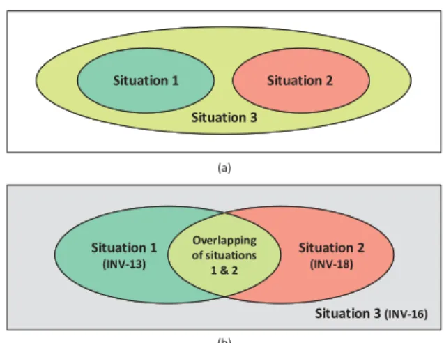
The situations addressed in an OR-decomposition may overlap, i.e., their charactering assumptions can hold at the same time. This is the case of INV-13 and INV-18 capturing that both one Firefighter is in danger and a nearby colleague as well. Consequently, there are more than one applicable configurations and therefore a prioritization is needed (Section 6.2). As an aside, allowing situations in an OR-decomposition to overlap also provides a built-in fault-tolerance mechanism (Section 10.1.1). Technically, if a design alternative in an OR-decomposition is further refined in terms of an AND-decomposition (or vice-versa), we omit the invariant representing the alternative and connect the AND-decomposition directly to the OR-decomposition to improve readability (e.g., design alternatives of INV-12).
We distinguish two kinds of invariants: computable and
non-computable. While a computable invariant can be
programmatically evaluated at runtime, a non-computable invariant serves primarily for design and review-based validation purposes. Thus, the characterizing assumptions need to be either computable or decomposed into computable assumptions. An example of a non-computable characterizing assumption is INV-16: “No life threat”. It is AND-decomposed into the computable assumptions INV-20 and INV-21, representing two orthogonal concerns, which can be evaluated by monitoring the Firefighter’s internal state.
Dependencies may also exist between invariants in design alternatives across different OR-decompositions (cross-tree
dependencies), reflecting constraints of the physical world. These
dependencies are captured in the IRM-SA model by directed links between invariants labeled with “requires”, resp. “collides”, which capture the constraint that the source invariant can appear in a configuration only with, resp. without, the target invariant. For example, in order for INV-32 to appear in a configuration, INV-30 has to be included as well, capturing the real-life constraint where the Personal Alert Safety System (PASS) is attached to the
self-contained breathing apparatus (SCBA) of a firefighter; thus if the
SCBA is not used, then the PASS cannot be used as well. The “collides” dependency is not illustrated in our running example.
5.2 Concepts Addressing Dependability
In IRM-SA, dependability is mainly pursued by tracing the low-level processes to high-low-level invariants. Moreover, to deal with the operational uncertainty in dynamic siCPS, IRM-SA goes beyond the classical goal-modeling approaches and allows self-adaptation based not only on valuations of belief (snapshot of a remote component’s internal data), but also on valuations ofFigure 2: IRM-SA model of the running example. + id + groupLeaderId + sensorData + position + temperature + acceleration + oxygenLevel + nearbyGMsStatus Firefighter + id + sensorDataList + GMInDanger Officer INV-2 GM::groupLeaderId==GL::id
INV-1 GL keeps track of the condition of his/her group’s members
INV-3 GL keeps track of the condition of the relevant members
INV-7 GM::nearbyGMInDanger – GMs’ belief of GL::GMInDanger – is updated every 4 secs
X INV-6 GL::GMInDanger > 0 X INV-8 GL::GMInDanger==0
INV-5 Up-to-date GL::sensorDataList, w.r.t. GM::sensorData, is available
INV-10 GL::sensorDataList - GL’s belief over the GM::sensorData – is updated every 2 secs
X INV-9 GM::sensorData is
determined
INV-18 Nearby GM in danger/critical state INV-13 GM in danger INV-15 GM::temperature is
monitored every 1 sec P
INV-11 GM::acceleration is monitored every 1 sec
P
INV-17 GM::temperature is monitored every 5 secs
P INV-19 AVG(GM::acceleration)==0 in past 20 sec INV-12 GM::position is determined
INV-16 No life threat
INV-14 GM::oxygenLevel is monitored when possible
INV-20 AVG(GM::acceleration)>0 in past 20 sec INV-21 GM:nearbyGMsStatus==OK INV-22 GM::nearbyGMsStatus==DANGER INV-29 Breathing apparatus is used
INV-28 Breathing apparatus is not used
INV-30 GM::oxygenLevel is monitored every 1 sec
P
INV-24 GM indoors INV-26 GM outdoors
INV-27 GM::position is determined from GPS every 1 sec
P INV-25 GM::position is
determined from indoors tracking system every 1 sec
P Subtree for
“Search and Rescue” situation INV-31 PASS alert is sounded
when needed
INV-32 PASS alert is sounded every 5 secs
P
requires
INV-23
possibility(GM::nearbyGMsStatus==CRITICAL) w INV-4 GL::GMInDanger is determined from the GL::sensorDataList every 4 secs
P *[GM] [GM] [GL] 1[GL] 1[GM] [GM] GroupMember role GroupLeader role [GL] Takes-role relation Invariant Process invariant Exchange invariant Assumption AND decomposit ion Component P X Dependency relation OR decomposit ion Characterizing Assumption
associated metadata (timestamp of belief, timestamp of sending/receiving the belief over the network, etc.). This functionality also adds to the dependability by self-adapting in anticipation of critical situations. Nevertheless, IRM-SA support for dependability does not cover other dependability aspects, such as privacy and security.
A key property here is that a belief is necessarily outdated, because of the distribution and periodic nature of real-time sensing in siCPS. For example, the position of a Firefighter as perceived by his/her Officer would necessarily deviate from the actual position of the Firefighter if he/she were on the move. Instead of reasoning directly on the degree of belief outdatedness (on the time domain), we rely on models that predict the evolution of the real state (e.g., state-space models if this evolution is governed by a physical process), translate the outdatedness from the time domain to the data domain of the belief (e.g., position inaccuracy in meters) and reason on the degree of belief
inaccuracy. We call this type of reasoning proactive reasoning.
To enable proactive reasoning, we build on our previous work in quantifying the degree of belief inaccuracy in dynamic siCPS architectures [1].
For illustration, consider an assumption “inaccuracy(GM:: position) < 20 m”, which models the situation where the difference of the measured and actual positions is less than 20 meters. In this case, belief inaccuracy is both (i) inherent to the sensing method (more GPS satellites visible determine more accurate position), and (ii) related to the network latencies when disseminating the position data (more outdated data yield more inaccurate positions – since firefighters are typically on the move, their position data are subject to outdating). As a result, an Officer has to reason on the cumulative inaccuracy of the position of his/her Firefighter.
When the domain of the belief field is discrete instead of continuous, we rely on models that capture the evolution of discrete values in time, such as timed automata. For illustration, consider assumption INV-23: “possibility(GM::nearbyGMsStatus == CRITICAL)”, which models the situation where the nearbyGMsStatus enumeration field with values OK, DANGER, and CRITICAL is possible to evaluate to CRITICAL. This presumes that the designer relies on a simple timed automaton such as the one depicted in Figure 3, which encodes the domain knowledge that a firefighter gets into a critical situation (and needs rescuing) at least 5 seconds after he/she gets in danger.
All in all, the invariants that are formulated with inaccuracy and
possibility provide a fail-safe mechanism for adversarial
situations, when the belief of a component gets so inaccurate that special adaptation actions have to be triggered. This proactive reasoning adds to the overall dependability of the self-adaptive siCPS.
5.3 The Modeling Process
Figure 3: Timed automaton capturing the transitions in the valuation of the nearbyGMsStatus field.
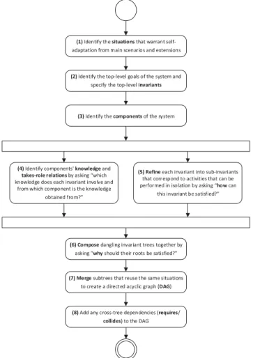
Figure 4: Steps in the IRM-SA modeling process.
Figure 5: Steps in a single invariant refinement. DANGER OK CRITICAL t>5 sec t:=0 t>0 sec
(1) Identify the situations that warrant self-adaptation from main scenarios and extensions
(4) Identify components' knowledge and takes-role relations by asking “which knowledge does each invariant involve and
from which component is the knowledge obtained from?”
(3) Identify the components of the system (2) Identify the top-level goals of the system and
specify the top-level invariants
(6) Compose dangling invariant trees together by asking “why should their roots be satisfied?”
(5) Refine each invariant into sub-invariants that correspond to activities that can be performed in isolation by asking “how can
this invariant be satisfied?”
(7) Merge subtrees that reuse the same situations to create a directed acyclic graph (DAG)
(8) Add any cross-tree dependencies (requires/ collides) to the DAG
Is it a process/invariant/exchange invariant/computable assumption?
[YES]
[NO]
OR-decompose invariant into sub-invariants
AND-decompose invariant into sub-invariants Specify the characterizing
assumption for each situation
[YES]
Does the invariant cover more than one situations? [NO]
As is usually the case with software engineering processes, IRM-SA modeling process is a mixed top-down and bottom-up process. As input, the process requires a set of use cases/user stories covering both the main success scenarios and the associated extensions. The main steps of the process are illustrated in Figure 4. After the identification of the main situations, goals and components, the architect starts to specify the knowledge of each component together with its takes-role relations (step 4), while, in parallel, he/she starts refining the invariants (step 5). These two steps require potentially several iterations to complete. In step 6, the architect composes the dangling invariant trees that may have resulted from the previous steps, i.e., the trees the roots of which are not top-level invariants. Contrary to the previous steps, this is a bottom-up design activity. In the final steps, as an optimization, the subtrees produced in the previous steps that are identical are merged together, and “requires”/“collides” dependencies are added. The result is a DAG – this optimization was applied also in Figure 2.
The workings of a single refinement are depicted in Figure 5. Based on whether the invariant under question is to be satisfied in a different way in different situations (e.g., “position reading” will be satisfied by using the GPS sensor when outdoors and by using the indoor positioning system when indoors), the architect chooses to refine the invariant by OR- or AND-decomposition. Obviously, in the former case, the refinement involves specifying the characterizing assumption for each design alternative (situation). Note that, if the characterizing assumption is not computable, it will get refined in a next step as any other invariant in such a case.
The process of systematic identification of all the possible variation points and modeling the corresponding design alternatives and situations is closely related to the identification of adaptation scenarios in a Dynamically Adaptive System (DAS) [32]. Here, one can leverage existing approaches in requirements engineering ranging from documentation of main use-case scenarios and extensions to obstacle/threat analysis on goal models [52]. Performance and resource optimization concerns can also guide the identification of variation points and corresponding design alternatives.
For example, the rationale behind the OR-decomposition of the left-most part of the AND-decomposition of INV-9 is resource optimization: under normal conditions the accuracy of external temperature monitoring can be traded off for battery consumption of the low-power node; this, however, does not hold in danger (e.g., a firefighter is not moving, INV-19), when higher accuracy of external temperature monitoring is needed.
On the contrary, the OR-decomposition of INV-12 has its rationale in a functional constraint: since GPS is usually not available within a building, a firefighter’s position has to be monitored differently in such a case, e.g., through an indoors tracking system [17]. This is an example of a technology-driven process of identification of design alternatives, where the underlying infrastructure significantly influences the possible range of adaptation scenarios [32]. For example, it would not make sense to differentiate between the situations of being indoors and outdoors, if there were no way to mitigate the “GPS lost signal” problem using the available infrastructure.
This highlights an important point: IRM-SA allows for modeling the environment via assumptions, but, at the same time, guides the designer into specifying only the pertinent features of the environment, avoiding over-specification.
For a complete example of this modeling process, we refer the reader to the online IRM-SA User Guide2. To support the
modeling process, we have also developed a prototype of a GMF-based IRM-SA design tool [42].
6. SELECTING ARCHITECTURE
CONFIGURATIONS BY SAT SOLVING
As outlined in Section 4, given an IRM-SA model, the selection of a configuration for a situation can be advantageously done by directly reasoning on the IRM-SA model at runtime. In this section we describe how we encode the problem of selecting an applicable configuration into a Boolean satisfiability (SAT) problem (6.1), our prioritizing strategy with multiple applicable configurations (6.2), and how we bind variables in the SAT instance based on monitoring (6.3).To simplify the explanation, we use the term “clause” in this section even for formulas which are not necessarily valid clauses in the sense of CNF (Conjunctive Normal Form – the default input format for SAT), but rely on the well-known fact that every propositional formula can be converted to an equisatisfiable CNF formula in polynomial time.
6.1 Applicable Configurations
Formally, the problem of selecting an applicable configuration is the problem of constructing a set of selected invariants from an IRM-SA model such that the following rules are satisfied: (i) all the top-level invariants are in ; (ii) if an invariant is decomposed by an AND-decomposition to , … , , then ∈ iff all , … , ∈ ; (iii) if an invariant is decomposed by an OR-decomposition to , … , , then ∈ iff at least one of , … , is in ; (iv) if an invariant requires, resp. collides (with), , then ∈ iff ∈ , resp. ∉ . The set C represents an applicable configuration. The rules above ensure that is well-formed with respect to decomposition and cross-tree dependencies semantics. Figure 6 shows a sample applicable configuration (selected invariants are outlined in grey background).
Technically, for the sake of encoding configuration selection as a SAT problem, we first transform the IRM-SA model to a forest by duplicating invariants on shared paths. (This is possible because the IRM-SA model is a DAG.) Then we encode the configuration
2 http://www.ascens-ist.eu/irm
Figure 6: An architecture configuration of the running example. 2 1 3 7 X 6 X 8 5 10 X 9 18 13 15 P 11 P 17 P 19 12 16 14 20 21 22 29 28 30 P 24 26 27 P 25 P 31 32 P requires 23 4 P
Process & Ensemble Invariants involved in the architecture configuration
we are looking for by introducing Boolean variables , … , , such that = iff ∈ . To ensure is well-formed, we introduce clauses over , … , reflecting the rules (i)-(iv) above. For instance, the IRM-SA model from Figure 2 will be encoded as shown in Figure 7, lines 1-26.
To ensure that is an applicable configuration w.r.t. a given situation, we introduce Boolean variables , … , and add a clause ⇒ for each ∈ {1 … } (Figure 7, line 29). The value of captures whether the invariant is acceptable; i.e., indicates that it can be potentially included in , indicates otherwise. The variables , … , are bound to reflect the state of the system and environment (Figure 7, lines 31-39). This binding is described in Section 6.3.
In the resulting SAT instance, the variable for each top-level invariant is bound to true to enforce the selection of at least one applicable configuration. A satisfying valuation of such a SAT instance encodes one applicable configuration (or more than one in case of overlapping situations – see Section 6.2), while unsatisfiability of the instance indicates nonexistence of an applicable configuration in the current situation.
6.2 Prioritizing Applicable Configurations
Since the situations in an OR-decomposition do not need to be exclusive but can overlap, SAT solving could yield more than one applicable configurations. In this case, we assume a post-processing process that takes as input the IRM-SA model with the applicable configurations and outputs the selected configuration based on analysis of preferences between design alternatives. For this purpose, one can use strategies that range from simple total preorder of alternatives in each decomposition to well-established soft-goal-based techniques for reasoning on goal-models [20]. In the rest of the section, we detail on the prioritization strategy used in our experiments, which we view as just one of the many possible.In our experiments (Section 7.2), we have used a simple prioritization strategy based on total preorder of design alternatives in each OR-decomposition. Here, for simplicity, a total preorder – numerical ranking – is considered (1 corresponds to the most preferred design alternative, 2 to the second most preferred, etc.). The main idea of the strategy is that the preferences loose significance by an order of magnitude from top to bottom, i.e., preferences of design alternatives that are lower in an IRM-SA tree cannot impact the selection of a design alternative that is above them on a path from the top-level invariant.
More precisely, given an IRM-SA tree, every sub-invariant of an OR-decomposition is associated with its OR-level number , which expresses that is a design alternative of a -th OR-decomposition on a path from the top-level invariant (level 1) to a leaf. For each OR-level, there is its cost base defined in the following way: (a) the lowest OR-level has cost base equal to 1, (b) the -th OR-level has its cost base = ∗ ( + 1), where denotes the number of all design alternatives at the level + 1 (i.e., considering all OR-decomposition at this level). For example, the 2nd OR-level in the running example has
= ∗ ( + 1) = 1 ∗ (4 + 1) = 5, since the 3rd OR-level (lowest) has in total 4 design alternatives (2 from the OR-decomposition of INV-14 and 2 from that of INV-18).
Having calculated the base for each OR-level, the cost of a child invariant of a -th OR-decomposition with a cost is defined as ∗ , where denotes the rank of the design
alternative that the invariant corresponds to. Finally, a simple graph traversal algorithm is the employed to calculate the cost of each applicable configuration as the sum of the cost of the selected invariants in the applicable configuration. The applicable configuration with the smallest cost is the preferred one – becomes the current configuration.
6.3 Determining Acceptability
Determining acceptability of an invariant (i.e., determining the valuation of ) is an essential step. In principle, a valuation of reflects whether is applicable w.r.t. the current state of the system and the current situation. Essentially, = implies that cannot infer an applicable configuration.
We determine the valuation of in one of the following ways (alternatively):
(1) Active monitoring. If belongs to the current configuration and is computable, we determine by evaluating w.r.t. the current knowledge of the components taking a role in .
(2) Predictive monitoring. If does not belong to the current configuration and is computable, it is assessed whether would be satisfied in another configuration if chosen.
In principle, if is not computable, its acceptability can be inferred from the computable sub-invariants.
For predictive monitoring, two evaluation approaches are employed: (a) The invariant to be monitored is extended by a
1. // 1. configuration constraints based of the IRM model
2. // top level decomposition in Figure 2
3. _ ∧ ∧ ⇔ // s _ represents the anonymous
invariant in the AND decomposition of INV-9
4. _ ∨ _ ∨ s ⇔ // s is a copy of s
5.
6. // decomposition level 1 in Figure 2
7. _ _ ∨ _ _ ∨ _ _ ⇔ _
8. _ ∨ _ ⇔
9. ∧ ⇔ _ // s is a copy of s
10.
11. // decomposition level 2 in Figure 2
12. ∧ ∧ ⇔ _ _ 13. ∧ ⇔ _ _ 14. ∧ … ⇔ _ _ 15. ∧ ⇔ _ 16. ∧ ⇔ _ 17.
18. // decomposition level 3 in Figure 2
19. ⇔ 20. ⇔ 21. _ ∨ ⇔ 22. ∧ ⇔ 23. … // similar for , 24.
25. // decomposition level 4 in Figure 2
26. ∧ ⇔ _
27.
28. // 2. only applicable invariants may be selected into a configuration
29. ( ⇒ ) ∧ … ∧ ( ⇒ ) ∧ …
30.
31. // 3. determining acceptability according to monitoring
32. // (current configuration as shown in Figure 6)
33. // 3.1. active monitoring
34. = ⋯ // true or false based on the monitoring of INV-9
35. … // repeat for , , , , , , , , , , , , ,
36.
37. // 3.2. predictive monitoring
38. = ⋯
39. … // repeat for the rest
Figure 7: Encoding the IRM-SA model of running example into SAT.
monitor predicate (which is translated into a monitor – Section
8.4) that assesses whether the invariant would be satisfied if selected, and (b) the history of the invariant evaluation is observed in order to prevent oscillations in current configuration settings by remembering that active monitoring found an invariant not acceptable in the past.
Certainly, (a) provides higher accuracy and thus is the preferred option. It is especially useful for process invariants, where the monitor predicate may assess not only the validity of process invariant (e.g., by looking at knowledge valuations of the component that take a role in it), but also whether the underlying process would be able to perform its computation at all. This can be illustrated on the process invariant INV-27, where the process maintaining it can successfully complete (and thus satisfy the invariant) only if GPS is operational and at least three GPS satellites are visible.
7. SOLVING THE SAT PROBLEM IN
DISTRIBUTED SETTINGS
When implementing self-adaptation via IRM-SA in a distributed siCPS such as the firefighter tactical decision system, there are three main choices to consider:
1. Centralized self-adaptation (CA). A selected arbiter collects all the necessary knowledge from components, solves the SAT problem, and reliably communicates the result back to the components. This assumes that the system can be paused for the whole duration of the above process (strict synchronization), so that each component receives self-adaptation decisions that are relevant to its current state. 2. Decentralized self-adaptation with distributed consensus
(DADC). Each component performs SAT solving locally
based on its local knowledge (local view of system state), without requiring this knowledge to be synchronized across components. The results of SAT solving are then communicated and agreed upon between all components. This relaxes the assumption on strict synchronization, but still assumes that a component can be paused from the point that it solves the SAT problem until a consensus is built. 3. Decentralized self-adaptation with no distributed consensus
(DANC). Similar to DADC, each component performs SAT
solving locally based on its local knowledge, (local view of system state), without requiring this knowledge to be synchronized across nodes. However, the results of SAT solving are not communicated and no consensus is built. This allows components to keep their autonomy even detached from the network.
CA and DADC are both well-known solutions, documented in the state of the art of distributed systems [27, 28], multi-agent systems and autonomous agents [43, 62], and cooperative and networked control systems [33, 36]; they are also widely used in practice. They work well in systems with limited dynamicity, where network communication and the consequent timing issues (e.g., delays) can be mostly ignored or bounded. These assumptions are however not plausible in many siCPS, which are spatial systems deployed on top of ad-hoc wireless infrastructures with no communication guarantees and comprised of components that can dynamically appear and disappear. In such contexts, DANC is a more fitting choice, as it can be easily combined with proactive reasoning (Section 5.2) at the level of each individual component. This combination allows each component to make individual decisions that can help deal with threats related to network disconnections and delays.
In the rest of this section we detail on DANC by identifying and formalizing the criteria that establish the perimeter of its applicability. We also exemplify the combination of DANC and proactive reasoning in our running example and discuss its ability to deal with threats related to network disconnections.
7.1 Decentralized Self-Adaptation with no
Distributed Consensus
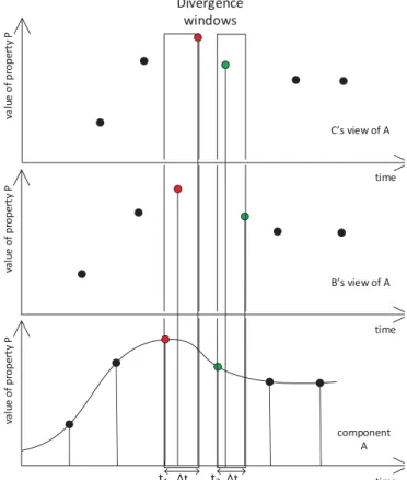
DANC can be employed in systems that are by nature resilient to situations when the system is synchronized. During de-synchronization, some nodes of the system arrive at different decisions due to their differently outdated knowledge (divergence). This can result into inconsistencies, e.g., cases where there are assumptions in the IRM-SA model that one component considers satisfied, while another considers violated. As an example, depicted in Figure 8, a property P of component A may reach some critical value (which invalidates an assumption) at time t1; this is observed only after some time (divergence
window Δt) in components B and C. A respective divergence window again exists in the case when P’s value falls back within a “normal” range. It is important to note that data outdatedness does not always lead to divergence, because though different, they can lead to the same decision – this can be observed in Figure 8 in the areas outside the two intervals.
DANC specifically targets systems where temporary divergence of the SAT solving input and, consequently, of its results has only negligible effect in the performance of the system (what is considered “negligible” in this case depends on particular domain requirements). This prerequisite characterizes the type of systems that can employ DANC – when it does not hold, CA or DADC has to be chosen instead.
time va lu e of pr ope rt y P t1 Divergence windows t2 component A B’s view of A C’s view of A Δt Δt time time va lu e of pr ope rt y P va lu e of pr ope rt y P
Figure 8: Connection between outdated views and divergence windows.
We formalize the above prerequisite and describe the criteria that imply it below. Figure 9 provides a graphical summary.
Definition 1 (Utility of a system run). For a given run of a
system:
– Let ( ) be a function that for time returns the set of active processes as selected by the SAT procedure.
– Let ( , ) be function that for time and a knowledge field returns the time Ǽ that has elapsed since the knowledge value contained in was sensed/created by the component where the knowledge value originated from.
– Let , ( ) be a function that for given time returns a set
of active processes of component as selected by the SAT procedure assuming that knowledge values outdated by ( , ) have been used. Further, we denote ,…, ( ) = ⋃ , ( ) as the combination over components existing in
the system. (In other words, each component selects active processes itself based on its belief, which is differently outdated for each component.)
– Let ( ) be a cumulative utility function that returns the overall system utility when performing processes ( ) at each time instant .
– Let ( , Δmax) be a cumulative utility function constructed
as min ,…, ( ) ≤ Δmax}. (In other words,
( , Δmax) denotes the lowest utility if components decide
independently based on knowledge at most Δ max old.)
Definition 2 (Expected relative utility). Let E( ( )) be the expected value of ( ) and E( ( , Δmax)) be the expected value
of ( , Δmax). Assuming that E ( ) > 0 (i.e., in the ideal case
of zero communication delays the system provides a positive value), we define expected relative utility as (Δmax) =
E ( , Δ max) /E ( ) .
We assume systems where (Δ max) is close to 1 (and definitely
non-negative) for given upper bound on communication delays Δmax. In fact (Δmax) provides a continuous measure of how
well the method works in a distributed environment.
Considering that the communication in the system happens periodically and that an arriving message obsoletes all previous not-yet-arrived messages from the same source, Δmax can be set to + , where is a close-to-100% quantile of the distribution of message latencies, is the period of message sending and is a close-to-100% quantile of the distribution of the length of sequences of consecutive message drops. Naturally, if there is a chance of some (not necessarily reliable communication), Δmax can be set relatively low while still
covering the absolute majority of situations.
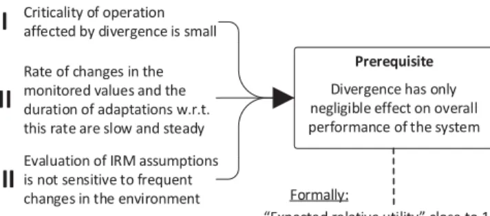
There are several factors that influence the value of (Δmax). Essentially, it depends on the shape of the utility function (since the utility function is cumulative), on the duration of divergence, and on the robustness of the utility function with respect to divergence. Following this argument, we identify three criteria for the applicability of IRM-SA with DANC. Essentially, “ (Δmax) close to 1” is achieved when:
Criticality of a particular system operation affected by divergence is small. For critical operations, the utility function
tends to get extreme negative values, thus even a short operation under divergence yields very low overall utility. On the other hand, if the environment has revertible and gradual responses, it hardly matters whether the system is in divergence for a limited time (e.g., if the system controls a firefighter walking around a building, then walking in a wrong direction for a few seconds does not cause any harm and its effect can be easily reverted).
Rate of changes in the monitored values and the duration of adaptations w.r.t. this rate are slow and steady. As the system
reacts to changes in the environment, it is impacted by the speed these changes happen. Such a change creates potential divergence in the system. What matters then is the ratio between the time needed to converge after the divergence and the interval between two consecutive changes. For instance, if house numbers were to be observed by firefighters when passaging by, then walking speed would yield much slower rate of changes then passing by in a car.
Evaluation of assumptions is not sensitive to frequent changes in the environment. This is a complementary aspect of the
previous property. Depending on the way assumptions are refined into computable ones, one can detect fine-grained changes in the environment. For example, consider an assumption that relies on computing position changes of a firefighter moving in a city. Computing position changes based on changes in the house number obviously yields more frequent (observable) changes in the environment than computing changes based on the current street number.
7.2 A Case for Decentralized Self-Adaptation
with no Distributed Consensus
We now provide a particular scenario where DANC is the most fitting choice, and exemplify the combination of DANC with proactive reasoning.
Consider the scenario where teams of firefighters consisting of three members and one leader were deployed. A firefighter A senses temperature higher than a pre-specified threshold (indication of being “in danger”); this information is propagated to the A’s leader who in turn propagates the information that A is in danger to a firefighter B; then, B performs self-adaptation in the anticipation of the harmful situation of having a group member in danger (proactive self-adaptation) and switches the mode to “Search and Rescue” (the situation captured by INV-18 in Figure 2). At the point when the leader determines that A is in danger (and just before the leader communicates it to B), a temporary network disconnection occurs. The overall performance was measured by reaction time – the interval between the time that A sensed high temperature and the time that B switches to “Search and Rescue”. Note that, by setting ( ) to be the inverse of the reaction time, we obtain values for the expected relative utility r that range from (1000) = = 0.37 to (12000) = = 0.15.
Criticality of operation affected by divergence is small Rate of changes in the monitored values and the duration of adaptations w.r.t. this rate are slow and steady Evaluation of IRM assumptions is not sensitive to frequent changes in the environment
I
II
III
Prerequisite
Divergence has only negligible effect on overall performance of the system
“Expected relative utility” close to 1 Formally:
We performed several simulations of the above scenario in order to delineate the limits of proactive self-adaptation. In particular, the questions that we investigated by the experiments were the following.
Q1: Do temporary network disconnections (and associated
communication delays) reduce the overall performance of an application that employs DANC?
Q2: Does proactive self-adaptation in IRM-SA method in
combination with DANC increase the overall performance of an application in face of temporary disconnections?
Simulation setup. In the experiments we employed an extended
version of the running example. This IRM-SA model of consists of 4 components, 39 invariants, and 23 decompositions [42]. The experiments were carried out using the jDEECo simulation engine [44] together with the prototype implementation of IRM-SA in jDEECo (Section 8). Several simulation parameters (such as interleaving of scheduled processes) that were not relevant to our experiment goals were set to fixed values. The simulation code, along with all the parameters and raw measurements, are available online [42].
To obtain a baseline, the case of no network disconnections was also measured. The result is depicted in dashed line in Figure 10. To investigate Q1 and Q2, a number of network disconnections with preset lengths were considered; this was based on a prior experience of working with deployment of DEECo on mobile ad-hoc networks [14].
To answer Q2, the timed automaton (Figure 3) associated with INV-23: “possibility(GM::nearbyGMsStatus == CRITICAL)” was modified: the transition from DANGER to CRITICAL was made
parametric to experiment with different critical threshold values – critical threshold in the context of the experiments is the least time needed for a firefighter to get into a critical situation after he/she gets in danger (in Figure 3 the critical threshold is set to 5 sec). The reaction times for different critical thresholds and different disconnection lengths are in Figure 10.
To answer Q1 (as well as obtain the baseline), the critical threshold was set to infinity – effectively omitting INV-23 from the IRM-SA model – in order to measure the vanilla case where self-adaptation is based only on the values of data transmitted (belief) and not on other parameters such as belief outdatedness and its consequent inaccuracy.
Analysis of results. From Figure 10 it is evident that the reaction
time (a measure of the overall performance of the system) strongly depends on communication delays caused by temporary disconnections. Specifically, in the vanilla case the performance is inversely proportional to the disconnection length, i.e., it decreases together with the quality of the communication links. This is in favor of a positive answer to Q1.
Also, to cope with operational uncertainty – temporary network disconnections in particular – the IRM-SA mechanisms are indeed providing a solution towards reducing the overall performance loss. Proactive self-adaptation yields smaller reaction times (Figure 10) – this is in favor of a positive answer to Q2. In particular, for the lowest critical threshold (2000ms) the reaction time is fast; this threshold configuration can, however, result into overreactions, since it hardly tolerates any disconnections. When setting the critical threshold to 5000ms, proactive self-adaptation is triggered in case of larger disconnections (5000ms and more) only. A critical threshold of 8000ms triggers proactive self-adaptation in case of even larger disconnections (8000ms or more). Finally, when critical threshold is set to infinity, proactive self-adaptation is not triggered at all.
When disconnection times grow larger and larger, proactive self-adaptation can help in bounding the amount of performance loss. In our case, predictions were based on the timed automaton of Figure 3; in case the possibility of a life-critical situation was predicted, the system switched to the “Search and Rescue” mode. Although several simplifying assumptions were made (e.g., a single, simple automaton was used, all predictions were assumed correct), the experiments provide evidence on the applicability of DANC with proactive self-adaptation within the frame of IRM-SA. Extending the monitoring and prediction capabilities of our framework is subject to future work.
8. PROTOTYPE IMPLEMENTATION
We implemented the self-adaptation method of IRM-SA as a plugin (publicly available [42]) into the jDEECo framework [44]. This framework is a realization of the DEECo component model [15, 48] . For developing components and ensembles, jDEECo provides an internal Java DSL and allows their distributed execution. To give a better insight in the prototype implementation, we briefly first overview jDEECo below and then describe the main points of the implementation of IRM-SA.8.1 DEECo Component Model
Dependable Emergent Ensemble of Components (DEECo) is component model (including specification of deployment and runtime computation semantics) tailored for building siCPS with a high degree of dynamicity in their operation. In DEECo,
components are autonomous units of deployment and
computation. Each of them comprises knowledge and processes. Knowledge is a hierarchical data structure representing the
Figure 10: Reaction times for different network disconnection lengths and different critical thresholds. The results for each case have been averaged for different DEECo component knowledge publishing periods (400, 500 and 600 ms).
0 5000 10000 15000 20000 25000 1000 3000 5000 8000 12000 re achtion time ( ms) disconnection length (ms) critical threshold: 2000 ms critical threshold: 5000 ms critical threshold: 8000 ms critical threshold: infinity no network disconnections
internal state of the component. A process operates upon the knowledge and features cyclic execution based on the concept of feedback loop [60], being thus similar to a process in real-time systems. As an example, consider the two DEECo components in Figure 11, lines 7-13 and 15-23. They also illustrate that separation of concerns is brought to such extent that individual components do not explicitly communicate with each other. Instead, interaction among components is determined by their composition into ensembles – groups of components cooperating to achieve a particular goal [23, 40] (e.g., PositionUpdate ensemble in Figure 11, lines 27-34). Ensembles are dynamically established/disbanded based on the state of components and external situation (e.g., when a group of firefighters are physically close together, they form an ensemble). At runtime, knowledge
exchange is performed between the components within an
ensemble (lines 32-33) – essentially updating their beliefs (Section 3).
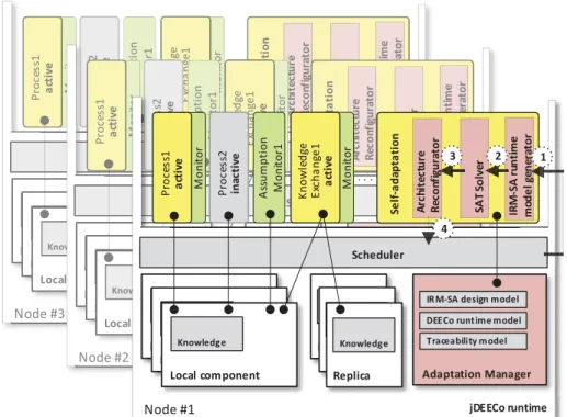
8.2 jDEECo Runtime
Each node in a jDEECo application contains a jDEECo runtime, which in turn contains one or more local components – serving as a container (Figure 13). The runtime is responsible for periodical scheduling of component processes and knowledge exchange functions (lines 12, 23, 34). It also possesses reflective capabilities in the form of a DEECo runtime model that provides runtime support for dynamic reconfigurations (e.g., starting and stopping of process scheduling). Each runtime manages the knowledge of both local components, i.e., components deployed on the same node, and replicas, i.e., copies of knowledge of the components that are deployed on different nodes but interact with the local components via ensembles.
8.3 Self-Adaptation in jDEECo
For integration of the self-adaptation method of IRM-SA
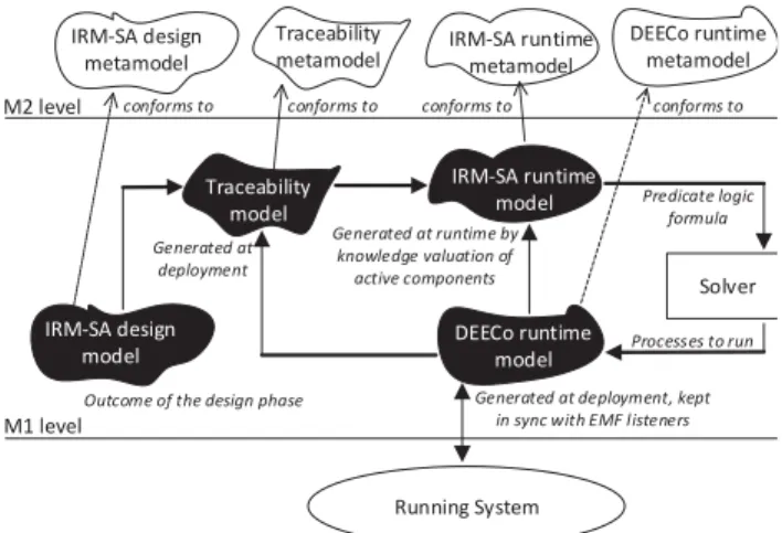
(jDEECo self-adaptation) with jDEECo, a models-at-runtime
approach [57] is employed, leveraging on EMF-based models (Figure 12). In particular, a Traceability model is created at deployment, providing the association of entities of the DEECo runtime model (i.e., components, component processes, and ensembles) with the corresponding constructs of the IRM-SA
design model (i.e., components and invariants). This allows
traceability between entities of requirements, design, and implementation – a feature essential for self-adaptation. For example, the process measurePositionGPS in Figure 11 is traced back to INV-27 (line 7), while the Firefighter component is traced back to its IRM-SA counterpart (line 2). Based on the Traceability model and the DEECo runtime model, an IRM-SA runtime model is generated by “instantiating” the IRM-SA design components with local components and replicas. Once the IRM-SA runtime model gets used for selecting an architecture configuration, the selected configuration is imposed to the DEECo runtime model as the current one.
A central role in performing jDEECo self-adaptation is played by a specialized jDEECo component Adaptation Manager (AM). Its functionality comprises the following steps (Figure 13): (1) Aggregation of monitoring results from local components and replicas and creation of IRM-SA runtime model. (2) Invocation of the SAT solver (Sections 6.1-6.3). (3) Translation of the SAT solver output into an applicable configuration (including prioritization). (4) Triggering the actual architecture adaptation – applying the current configuration. As an aside, internally, AM employs the SAT4J solver [53], mainly due to its seamless integration with Java.
The essence of step (4) lies in instrumenting the scheduler of the jDEECo runtime. Specifically, for every process, resp. exchange invariant in the current configuration, AM starts/resumes the scheduling of the associated component process, resp. knowledge exchange function. The other processes and knowledge exchange functions are not scheduled any more.
8.4 Monitoring
AM can handle both active and predictive monitoring techniques (Section 6.3). In the experiments described in Section 7.2, predictive monitoring was used for both component processes and knowledge exchange functions (based on observing the history of
1. role PositionSensor: 2. missionID, position 3. 4. role PositionAggregator: 5. missionID, positions 6.
7. component Firefighter42 features PositionSensor, …: 8. knowledge:
9. ID = 42, missionID = 2, position = {51.083582, 17.481073}, …
10. process measurePositionGPS (out position):
11. position ← Sensor.read()
12. scheduling: periodic( 500ms )
13. … /* other process definitions */ 14.
15. component Officer13 features PositionAggregator, …: 16. knowledge:
17. ID = 13, missionID = 2, position = {51.078122, 17.485260},
18. firefightersNearBy = {42, …}, positions = {{42, {51.083582,
19. 17.481073}},…}
20. process findFirefightersNearBy(in positions, in position, out
21. firefightersNearBy):
22. firefightersNearBy← checkDistance(position, positions)
23. scheduling: periodic( 1000ms )
24. … /* other process definitions */
25. … /* other component definitions */
26. 27. ensemble PositionUpdate: 28. coordinator: PositionAggregator 29. member: PositionSensor 30. membership: 31. member.missionID == coordinator.missionID 32. knowledge exchange:
33. coordinator.positions ← { (m.ID, m.position) | m ∈ members }
34. scheduling: periodic( 1000ms )
35. … /* other ensemble definitions */
Figure 11: Example of possible DEECo components and ensembles in the running example.
Figure 12: Models and their meta-models employed for self-adaptation in jDEECo.
Solver
Running System
Generated at deployment, kept in sync with EMF listeners Generated at deployment Generated at runtime by knowledge valuation of active components Processes to run Predicate logic formula DEECo runtime metamodel IRM-SA runtime metamodel Traceability metamodel IRM-SA design metamodel conforms to conforms to conforms to conforms to Traceability model IRM-SA runtime model DEECo runtime model IRM-SA design model M1 level M2 level