Localization of Single Link-Level Network Anomalies

HAL Id: hal-01183348

https://hal.archives-ouvertes.fr/hal-01183348

Submitted on 7 Aug 2015

HAL is a multi-disciplinary open access

archive for the deposit and dissemination of

sci-entific research documents, whether they are

pub-lished or not. The documents may come from

teaching and research institutions in France or

abroad, or from public or private research centers.

L’archive ouverte pluridisciplinaire HAL, est

destinée au dépôt et à la diffusion de documents

scientifiques de niveau recherche, publiés ou non,

émanant des établissements d’enseignement et de

recherche français ou étrangers, des laboratoires

publics ou privés.

Localization of Single Link-Level Network Anomalies

Emna Salhi, Samer Lahoud, Bernard Cousin

To cite this version:

Emna Salhi, Samer Lahoud, Bernard Cousin. Localization of Single Link-Level Network

Anoma-lies. International Conference on Computer Communication and Networks (ICCCN 2012), Jul 2012,

Munich, Germany. �10.1109/ICCCN.2012.6289247�. �hal-01183348�

Localization of Single Link-Level Network

Anomalies

Emna Salhi

Samer Lahoud

Bernard Cousin

Abstract—Achieving accurate, cost-efficient, and fast anomaly localization is a highly desired feature in computer networks. Prior works, examining the problem of single link-level anomaly localization, have shown that resources that enable the moni-toring of a set of paths distinguishing between all links of the network pairwise must be deployed for unambiguous anomaly localization. In this paper, we show that the number of pair of links that are to be distinguished can be cut down drasti-cally using an already established anomaly detection solution. This results in reducing the localization overhead and cost significantly. Furthermore, we show that all potential anomaly scenarios can be derived offline from the anomaly detection solution. Therefore, we compute full localization solutions, i.e. monitors that are to be activated and paths that are to be monitored, for all potential anomaly scenarios offline. This results in a significant minimization of localization delay. We devise an anomaly localization technique that selects monitor locations and monitoring paths jointly; thereby enabling a trade-off between the number and locations of monitoring devices and the quality of monitoring paths. The problem is formulated as an integer

linear program (ILP), and is shown to be N P-hard through a

polynomial-time reduction from the N P-hard facility location

problem. The effectiveness and the correctness of the proposed anomaly localization scheme are verified through theoretical analysis and extensive simulations.

Index Terms—Network monitoring, anomaly localization, anomaly detection, link-level anomalies.

I. INTRODUCTION

Anomaly localization aims at identifying unambiguously the link that causes an anomalous behavior of the network (e.g. excessive delay, high packet loss rate, etc.). It has long been combined with anomaly detection (e.g. [1]-[5]). How-ever, several research works argued that continuous anomaly localization can result in high overhead on the underlying network, and therefore, can interfere with the network ser-vices leading to service troubles. Recent works on network monitoring consider anomaly localization as a reaction to anomaly detection and perform two-phase monitoring (e.g. [6]-[12]). The first phase, the anomaly detection phase, uses as few network resources as possible to only detect anomalies. A necessary and sufficient condition to detect all link-level anomalies is to cover all the network links. Upon detecting an anomaly, the detection phase returns a set of suspect links.

This work was supported by Alcatel-Lucent Bell Labs France, under the grant n. 09CT310-01

Here comes the localization phase that aims at reducing the set of suspect links to the anomalous link(s). Clearly, this reactive anomaly localization approach reduces significantly the monitoring overhead compared to continuous anomaly localization. However it presents a serious challenge: the

localization must be as fast as possible, in order to enable a fast recovery of the network.

Argawal et al. [7] proposed an accurate link-level anomaly localization scheme that can localize all potential single link-level anomalies in a given network. The key idea is to deploy resources that enable the monitoring of a set of paths distinguishing all links of the network pairwise. Whenever an anomaly is detected, this set of paths is monitored in order to pinpoint the anomalous link. More recently, Barford et al. [8] proposed another scheme that selects paths that are to be monitored during the localization phase. Although this technique minimizes the localization overhead, because the monitored paths distinguish only between the suspect link, it suffers from two imperfections. The first is the non-negligible time of computing the set of paths that are to be monitored upon detecting an anomaly, which increases the localization delay (i.e. time elapsed between the moment when an anomaly is detected and the moment when the anomalous link is pinpointed). The second is that there is no guarantee to localize all potential anomalies, because deployed monitors ensure only the coverage of links. In this paper, we demonstrate that 1) not all links of the network need to be distinguishable pairwise towards localizing all potential anomalies, 2) all potential anomaly scenarios can be derived offline from any detection solution that covers all the network links. Thus, we compute full low-cost localization solutions, i.e. monitors that are to be activated and paths that are to be monitored, for all potential anomalies offline. Subsequently, we achieve an important gain in localization delay and overhead.

Furthermore, most existing works consider only one crite-rion for monitoring path selection that is the minimization of the number of monitored paths, and only one criterion for monitor location selection that is the minimization of the number of deployed monitoring devices. However, these criteria do not reflect the localization cost properly. Indeed, to reduce localization delay and overhead, monitoring of links that do not provide extra localization information during

the localization phase must be avoided. Moreover, monitor locations must be selected carefully towards minimizing the delay of communications between the Network Operation Center (NOC) and the deployed monitors. A novel anomaly localization cost model that considers the infrastructure cost, the localization overhead and the localization delays is, there-fore, proposed in this paper. Besides, our anomaly localization scheme selects monitor locations and monitoring paths jointly, thereby enabling a trade-off between the number and locations of deployed monitoring devices and the quality of selected monitoring paths. We formulate our scheme as an ILP, and we show that the problem is N P-hard through a polynomial-time reduction from the facility location problem.

We verify the effectiveness of our anomaly localization scheme by comparing it with existing anomaly localization schemes through extensive simulations

II. NETWORKMODEL ANDPROBLEMSTATEMENT

We model the network as a undirected graph G = (N , E) comprising a set of nodesN connected by a set of undirected links in E. Let P be the set of all non-looping paths of the network. Unless otherwise mentioned, without loss of generality, we assume that all the network paths are candidate to be monitored and all the network nodes are candidate to hold monitoring devices. We use the term monitoring paths to designate paths that are monitored during the detection phase, also referred to as detection paths, or during the localization phase, also referred to as localization paths. We denote the anomaly detection solution by (Dm,Dp). Dm is the set of

monitor locations where to deploy monitoring devices.Dpis a

set of monitoring paths traveling between the selected monitor locations and covering all the network links, ∪p∈Dpp = E.

We assume that an anomaly on link e ∈ E affects all the monitoring paths that cross e. Two links are said to be distinguishable from each other if we are able to decide which one is anomalous when an anomaly occurs on one of them.

We address the problem of single-link level anomaly lo-calization. The objective is to enable the localization of all potential link-level anomalies accurately; while minimizing the cost of acquiring and deploying monitoring devices, the localization overhead and the localization delay. Our localiza-tion scheme infers all potential anomaly scenarios from any detection solution that covers all links of the network. This has two major benefits. The first is that we pre-compute full localization solutions for all anomaly scenarios offline, thereby accelerating the localization process. The second is that we do not need to deploy resources that can distinguish every single pair of the network links. This is because, as it will be demonstrated in the next sections, only links that belong to the same anomaly scenario need to be distinguishable pairwise. The inputs into our localization problem are an instance of the graph G = (N , E) and a set of detection paths Dp

that can cover all links in E, and the outputs are a set of monitor locations whose monitors are to be activated and a set of paths that are to be monitored for each potential

anomaly. The localization solution must achieve a good trade-off between the monitor deployment cost, the localization overhead and the localization delay. To this end, a novel cost model that measures these three metrics is proposed. Also, our localization scheme selects monitor locations and localization paths jointly; as opposed to existing schemes that apply a two-step selection procedure, therefore omitting the trade-off between the number and locations of monitors and the quality of localization paths.

III. NOT ALL LINK PAIRS NEED TO BE DISTINGUISHABLE FOR LOCALIZING ALL SINGLE LINK-LEVEL ANOMALIES

In this section, we first establish a necessary and sufficient condition to distinguish between two links; and then, we prove that we do not need to distinguish between all links of the network pairwise in order to ensure accurate localization of all potential single link-level anomalies. This excludes a pre-established condition claiming that all links of the network need to be distinguishable pairwise in order to localize all potential single links level anomalies [7][8].

Theorem 1: The necessary and sufficient condition for two links e1 and e2 to be distinguishable from each other is the

existence of a monitoring path that crosses either e1 or e2,

but not both.

Proof: We first demonstrate the sufficiency condition.

Assume that either e1 or e2 is anomalous. Let p be a path

that crosses e1 (interchangeably e2) but not e2. If p exhibits

an anomaly, then the anomalous link must be crossed by p. We conclude that e1 is the anomalous link. If, p does not

exhibit an anomaly, then all links that are crossed by p are not anomalous. It follows that the anomalous link is e2. Thus,

p is sufficient to distinguish between e1 and e2.

The necessary condition can be proved as follows. Assume that it does not exist any path that crosses only one of the two links. Then, the monitoring path set can be divided into two types of paths: paths that cross both e1 and e2, and paths that

neither cross e1nor e2. An anomaly on a given link affects all

the monitoring paths that cross that link. Therefore, the latter type of paths is not affected by the anomalies on the two links, whereas the former type of paths is affected by the anomalies on the two links. Thus, the set of monitoring paths that are affected by an anomaly on e1is exactly the same set of paths

that is affected by an anomaly on e2. This means that e1 and

e2 cannot be distinguished from each other.

Existing localization schemes (e.g. [7], [8]) claim that all links of the network must be distinguished pairwise in order to localize all potential anomalies. According to Theorem 1, this means that ∀e1, e2 ∈ E there exists a monitoring

path that crosses either e2 or e2, but not both. However, we

will demonstrate that this is a sufficient but not necessary condition for localizing all potential anomalies, and we show how to infer the minimal set of pair of links that are to be distinguished from a given detection solution that covers all the network links.

Consider a network link e∈ E. We denote by De+and De−

the set of detection paths that cross e and the set of detection paths that do not cross e, respectively. The set of suspect links for an anomaly e is the set of potential anomalous links that is returned by the detection process when an anomaly occurs on link e, i.e. all links that the detection paths cannot distinguish from e.

Theorem 2: The set of suspect links for an anomaly on a given link e∈ E equals ∩p∈D_e+p− ∪p∈D_e−p.

Proof: We prove this theorem by construction. The set of

detection paths can be divided into two sets:

• De+: paths that cross link e.

• De−: paths that do not cross link e.

An anomaly on link e affects only paths that cross this link. Subsequently, paths in De₋ do not exhibit an anomaly.

It follows that all the links that are crossed by paths in De₋

are not suspect. Now, let L be the set of links that are crossed by paths in De+ and that are not crossed by paths in De−, L

=∪p∈D_e+p -∪p∈D_e−p . L can be divided into two subsets of

links:

• L1: links /∈ ∩p∈D_e+p− ∪p∈D_e−p • L2: links ∈ ∩p∈D_e+p− ∪p∈D_e−p

We prove by contradiction that all links in L1 are not

suspect. Assume to the contrary that a link l ∈ L1 is

suspect. This means that there does not exist any path in De+

that distinguishes between l and e. It follows that for each

p∈ De+, p crosses e and l. Thus l∈ ∩p∈De+p− ∪p∈De−p,

leading to a contradiction.

Likewise, we prove by contradiction that all links in L2

are suspect. Assume to the contrary that a link l ∈ L2 is

not suspect, then, there exists at least one path p ∈ De+

such that p distinguishes between e and l. Since all paths in De+ cross e, then p does not cross l. It follows that

l /∈ ∩p∈D_e+p− ∪p∈D_e−p, leading to a contradiction.

Corollary 1: A sufficient and necessary condition

to localize all potential link-level anomalies is to

distinguish each link e ∈ E from links that belong to

∩p∈D_e+p− {∪p∈D_e−p∪ {e}}.

We refer to the set of suspect links for an anomaly on link

e asS(e).

Corollary 2: e1∈ S(e2)⇔ S(e1) = S(e2),∀e1, e2∈ E

Corollary 3: S(e1)6= S(e2)⇔ S(e1)∩ S(e2) =∅

Let dS be the set of distinct sets of suspect links.

Corollary 4: ∪e_∈ES(e) = ∪_S(i)∈dSS(i) = E

Corollary 5: ∑_S(i)∈dS| S(i) | = | E |

Let AllP airs denotes the number of all the network link pairs. Clearly, AllP airs = (| E | ∗(| E | −1))/2. Let dP airs denotes the number of pair of links that need be distinguishable in order to localize all potential link-level anomalies.

Corollary 6: dP airs = AllP airs - X

S(i),S(j)∈dS:i<j

| S(i) | ∗ | S(j) |

The properties presented in the above corollaries are demon-strated in Appendix A. Corollary 6 confirms that we do not need to distinguish between all the network link pairs; unless the number of detection paths equals 1, which is very unlikely. It will demonstrated later in this paper that this reduction in the number of links pairs that are to be distinguished achieves great savings in resources needed to localize anomalies.

IV. DERIVATION OF POTENTIAL ANOMALY SCENARIOS

Theorem 2 states that the set of suspect links returned at the end of the detection phase whenever an anomaly on link e occurs is ∩p∈D_e+p− ∪p∈D_e−p. Therefore, instead of

computing monitors that are to be activated and paths that are to be monitored during the localization phase whenever an anomaly is detected, we propose to perform these compu-tations for all potential anomalies only once offline. Having a set of detection paths that cover all links of the network, we infer the set of suspect links for each link as described in Theorem 2. Then, a single anomaly scenario is created for all links that have the same set of suspect links, i.e. an anomaly scenario is created for each distinct set of suspect links. Let us denote by A the set of all anomaly scenarios, and let Sa denotes the set of suspect links associated to the

anomaly scenario a ∈ A. dS = {Sa,∀a ∈ A}. Clearly, the

least upper bound of the number of anomaly scenarios is the number of the network links. It is easy to show that when this bound is reached, the set of suspect links for an anomaly on link e, ∀e ∈ E, is reduced to the link e. In such case, the localization of all potential anomalies is immediate from the detection information. According to Corollary 2, we need to deploy monitors that enable the monitoring of a set of paths distinguishing links of each anomaly scenario pairwise in order to ensure the localization of all potential anomalies.

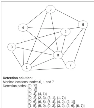
To illustrate, consider the sample network topology depicted in Fig. 1. An associated anomaly detection solution that covers all links of the network is depicted at the bottom of the figure. We use Theorem 2 to compute the set of suspect links for each link of the network. The result is depicted in Table I. The sets of suspect links associated to link (2, 3) and link (0, 7) are unitary. In case an anomaly occurs on one of these two links, there is no need to trigger the localization phase because the anomalous link is immediately pinpointed by intersecting the detection paths that exhibit the anomaly. Furthermore, four non-unitary anomaly scenarios (a1, a2, a3, a4) are created for

this topology (see table II). These are the four distinct non-unitary sets of suspect links. It should be noted that for this sample topology only 24 link pairs (P_1≤i≤4(| ai | ∗(| ai |

−1))/2) among the 153 link pairs of the network ( 18∗ (18 − 1)/2) need to be distinguishable.

V. ANOMALY LOCALIZATION COST

Consider a set of candidate monitor locations,M, a set of network paths that are candidate to be monitored,P0, and a set of anomaly scenarios A. The anomaly localization cost includes two costs:

Fig. 1:Illustrative network and an associated anomaly detection solution

TABLE I: Sets of suspect links for all potential anomalies

Anomalous link Set of suspect links

(0, 1) {(0, 1)} (0, 2) {(0, 2), (1, 3), (1, 7)} (1, 2) {(0, 6), (5, 6), (4, 5), (2, 4), (1, 2)} (0, 3) {(1, 5), (0, 5), (0, 3), (2, 6), (6, 7)} (1, 3) {(0, 2), (1, 3), (1, 7)} (2, 3) {(2, 3)} (0, 4) {(0, 4), (1, 4)} (1, 4) {(0, 4), (1, 4)} (2, 4) {(0, 6), (5, 6), (4, 5), (2, 4), (1, 2)} (0, 5) {(1, 5), (0, 5), (0, 3), (2, 6), (6, 7)} (1, 5) {(1, 5), (0, 5), (0, 3), (2, 6), (6, 7)} (4, 5) {(0, 6), (5, 6), (4, 5), (2, 4), (1, 2)} (0, 6) {(0, 6), (5, 6), (4, 5), (2, 4), (1, 2)} (2, 6) {(1, 5), (0, 5), (0, 3), (2, 6), (6, 7)} (5, 6) {(0, 6), (5, 6), (4, 5), (2, 4), (1, 2)} (0, 7) {(0, 7)} (1, 7) {(0, 2), (1, 3), (1, 7)} (6, 7) {(1, 5), (0, 5), (0, 3), (2, 6), (6, 7)}

TABLE II: Anomaly scenarios

Anomaly scenario Set of suspect links

a1 Sa1 ={(0, 2), (1, 3), (1, 7)}

a2 Sa2 ={(0, 6), (5, 6), (4, 5), (2, 4), (1, 2)}

a3 Sa3 ={(1, 5), (0, 5), (0, 3), (2, 6), (6, 7)}

a4 Sa1 ={(0, 4), (1, 4)}

• Monitor cost: it includes the effective cost of acquiring hardware and software monitoring devices and the cost of their maintenance. In addition, it includes the cost of communications between monitors and the NOC. For instance, the cost of communications between a monitor and the NOC can be expressed as a function of the physical distance that separates them. Let us denote by

Cnthe cost of deploying a monitor on node n. Let Ynbe a

binary variable that indicates whether node n is selected to hold a monitoring device. The monitor cost can be expressed as follows:

∑

n∈M

CnYn (1)

• Probe cost: it expresses the overhead of monitoring flows on the underlying network. Measurements of links that do not provide localization information should be avoided in order to minimize the monitoring overhead. Clearly, measuring links that do not belong to the set of suspect links of an anomaly scenario does not provide any extra localization information. Furthermore, measurement of links that belong to the set of suspect links might be useless. Revisit Fig. 1 and table I to illustrate. Consider an anomaly on link(6, 7). The associated set of suspect links is Sa3 ={(1, 5), (0, 5), (0, 3), (2, 6), (6, 7)}. Consider now

the set of paths {p1:(1, 5)(5, 6)(2, 6); p2:(1, 5)(0, 5)(0, 2);

p3:(1, 7)(6, 7)(2, 6)} that distinguishes between all the

suspect links pairwise. Path p1dividesSinto two subsets:

S1

a3{(1, 5), (2, 6)} and S

2

a3{(0, 5), (0, 3), (6, 7)}. The links

ofS1

a3are distinguished from links ofS

2

a3. Link(5, 6)that

is crossed by p1 does not belong to Sa3, and therefore,

it does not provide any localization information. Path p2

dividesS1

a3 into two subsets:S

11

a3{(1, 5)}andS

12_{{(2, 6)},}

and divides S2

a3 into two subsets: S

21

a3{(0, 5), (6, 7)} and

S22

a3{(0, 3)}. Finally, p3 distinguishes betwen (0, 5) and

(6, 7). However, it crosses (2, 6) that is already

distin-guished from all the other suspect links. Thus, measuring

(2, 6)by p3 does not provide extra localization

informa-tion, although it belongs toS.

Let us denote by Ce the cost of measuring link e. Ce

should be proportional to the load of link e, in order to avoid multiple measurements of the most overloaded links of the network. Consider an anomaly scenario a∈

A. Let us denote by Sathe set of suspect links associated

to the anomaly scenario a. Let Xpabe a binary variable

that specifies whether path p is part of the localization solution of a. Let δpe be a binary input parameter that

indicates whether path p crosses link e. The probe cost of the localization solution of a reads as follows:

∑

e_∈E,p∈P0

CeδpeXpa (2)

VI. ILP FORMULATION

The objective of the ILP is to find a localization solution for each anomaly scenario inA such that the anomaly localization cost is minimized. Let δpnbe a binary parameter that indicates

whether node n is an end-node of path p. For simplicity of notation, we define the following sets:

• δ_P0 ={δpe; p∈ P 0 , e∈ E} • δ_M={δpn; p∈ P 0 , n∈ M} • C_M={Cn; n∈ M} • C_E ={Ce; e∈ E}

Let α be the weight associated to the monitor cost, and let β be the weight associated to the probe cost. The input into the ILP is an instance of the graph G = (E, M, P0,A, δ_P0, δ_M, C_M, C_E, α, β). The objective function

minimizes the sum of the monitor cost and the probe cost. It reads as follows: α ∗ ∑ n∈M CnYn + β ∗ ∑ a∈A,e∈E,p∈P0 CeδpeXpa (3)

The ILP is subject to two constraints. The first constraint ensures that the end nodes of all selected monitoring paths hold monitoring devices. It reads as follows:

Yn≥ δpnXpa; ∀n ∈ M, ∀p ∈ P

0

,∀a ∈ A (4)

The second constraint ensures that the suspect links asso-ciated to each anomaly scenario are distinguishable pairwise. To this end, according to Theorem 2, the constraint ensures that for each anomaly scenario a and for each pair of suspect links (e1, e2) : e1, e2∈ Sa there exists at least one monitoring

path that crosses either e2 or e2, but not both. This constraint

reads as follows: ∑

p∈P0

(δpe1+ δpe2− 2δpe1δpe2)Xpa> 0;

∀a ∈ A; ∀e1, e2∈ Sa (5)

We show that the above inequality is sufficient to distinguish between all the link pairs of each anomaly scenario using the argument of the following theorem.

Theorem 3: Let P1 be the subset of paths of P

0 that cross either e1 or e2, but not both.

∑

p∈P0(δpe1 + δpe2 −

2δpe1δpe2) =| P1|.

Proof: Refer to Appendix B.

Corollary 7: If ∑_p∈P0(δpe1+ δpe2− 2δpe1δpe2)Xpa> 0,

then there exists at least one path in P0 that crosses either e1 or e2, i.e. there exists at least one path in P

0 that distinguishes between e1 and e2.

VII. OURANOMALYLOCALIZATIONPROBLEM IS

N P-HARD

Theorem 4: The anomaly localization problem presented in the previous section is N P-Hard.

Proof: Our anomaly localization problem can be reduced

from theN P-Hard facility location problem.

Facility location problem: consider a set of potential facility locationsF, and a set of clients D. Opening a facility at location i incurs a non-negative cost that is equal to fi. The

cost of servicing client j ∈ D by a facility installed at location

i ∈ F is dij. The problem is to find an assignment of each

client to exactly one facility such that the sum of the facility opening costs and the service costs is minimized.

We denote by f the set of facility opening costs, f = {fi, i ∈ F}, and by d the set of service costs, d =

{dij; i ∈ F, j ∈ D}. Given an instance I = (D, F, f, d)

of the facility location problem, we produce an instance

R(I) = (E, M, P0,A, δ_P0, δ_N, C_M, C_E, α, β) of our

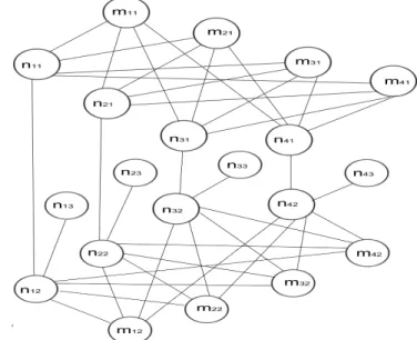
local-ization problem as follows. For each client j∈ D, we create:

• Three nodes labeled by nj1, nj2, and nj3. • One link connecting nj1 to nj2, labeled by ej1. • One link connecting nj2 to nj3, labeled by ej2. • An anomaly scenario aj such that Saj = {ej1, ej2}.

For each facility location i ∈ F, we create two nodes labeled by mi1 and mi2. For each i ∈ F and for each

j ∈ D, we create one link connecting mi1 to nj1, labeled

by e1

ij, and one link connecting mi2 to nj2, labeled by e2ij.

We obtain a graphG = (E, N ), where N = {nik; i∈ D, k ∈

[1; 3]} ∪ {mjk; i∈ F, k ∈ [1; 2]}, and E = {ejk; j∈ D, k ∈

[1; 3]}∪{ek

ij; i∈ F, j ∈ D, k ∈ [1; 2]}. An example of a graph

constructed out of a facility location instance with four facility locations and four clients is shown in Fig. 2.

Fig. 2: Example of a graph constructed out of a facility location instance with four facility locations and four clients

The candidate monitor location set is M = {mjk; i ∈

F, k ∈ [1; 2]}. The anomaly scenario set is A = {aj; j∈ D}.

The set of candidate monitoring paths isP0 ={pij; i∈ F, j ∈

D}, where pij is the non-looping path between mi1 and mi2

that crosses the links e1

ij, ej1and e2ij. The monitor deployment

costs are defined as follows: Cmi1 = Cmi2 = fi/2. The link

measurement costs are defined as follows: Cei1 = Cei2 = 0, Ce1

ij = Ce2ij = dij/2. The remaining input parameters can be

inferred easily fromG, M, A and P0 as follows:

• δajej0 k = { 1 if j = j0 0 otherwise ; ∀j, j 0 ∈ D, k ∈ [1; 2] • δ_ajek ij = 0; ∀i ∈ F, j ∈ D, k ∈ [1; 2] • δpijmi0 k= { 1 if i = i0 0 otherwise ; ∀i, i 0 ∈ F, k ∈ [1; 2] • δpijej1 = δpije1ij = δpije2ij = 1; ∀i ∈ F, j ∈ D • δpijej2 = 0; ∀i ∈ F, j ∈ D • α = β = 1

Obviously, the above reduction can be carried out in polynomial-time. In the sequel, we show that there is an

optimal solution to the Instance I of the facility location problem if and only of there is an optimal solution to the instance R(I) of our anomaly localization problem.

Let us start by demonstrating that if there is an optimal solution to the facility location instance, then there is a feasible solution to the anomaly localization instance. Let the facility location solution assigns each client j to a facility installed at location i. Consider the anomaly localization solution that selects for each anomaly scenario aj the path pij and the

monitor locations mi1 and mi2. Fix an anomaly scenario aj.

By construction, path pij crosses three links that are ej1and

e1

ij and e2ij . It follows, according to Theorem 1, that pij

distinguishes between ej1 and ej2. Constraint (4) states that

if pij is selected to be monitored, then, its end nodes must

be selected to hold monitoring devices. Thus, the solution that selects for each anomaly scenario aj the path pij to

be monitored, and its end nodes, mi1 and mi2, as monitor

locations is a feasible solution to the anomaly localization instance.

Conversely, we demonstrate that if there is an optimal solution to the anomaly localization instance, then there is a feasible solution to the facility location instance. An optimal solution to the facility location problem selects exactly one path for each anomaly scenario. This is because each anomaly scenario comprises only two links, and thus, monitoring one path that crosses exactly one of the two links is sufficient to distinguish between them. Let the optimal anomaly localiza-tion solulocaliza-tion selects for each anomaly scenario ajthe path pij,

and naturally, the monitor locations mi1 and mi2. Trivially,

the solution that assigns to each client j ∈ D the facility installed at location i is a feasible solution to the facility location instance.

We now prove that the constructed anomaly localization solution has the same cost as its corresponding optimal facility location solution (the proof holds in the converse case). Let Wi

and Zij be a binary variable that indicates whether a facility

is installed at location i, and a binary variable that indicates whether client j is serviced by a facility installed at location

i, respectively. Using the arguments that Zij = Xpijaj and Wi = Yi1 = Yi2, we show that the cost of the localization

solution, denoted by Cost(S_R(I)), is equal to the cost of its corresponding facility location solution, denoted by Cost(S_I), as follows: Cost(S_R(I)) = X mik∈M CmikYmik + X aj∈A,pij∈P0 (Ce1 ij + Ce2 ij)Xpijaj = X mi1∈M fiYmi1+ X aj∈A,pij∈P0 dijXpijaj =X i∈F fiWi+ X j∈D,i∈F dijZij = Cost(SI)

Now, we show that the solution to the anomaly localization instance, denoted by SR(I), that is constructed out of an

optimal solution to the facility location instance, denoted by

S∗_I, is optimal. Assume to the contrary that SR(I) is not

optimal. Let S_R(I)0∗ be an optimal solution to the anomaly

lo-calization instance, and let S_I0 be the facility location solution constructed out of S_R(I)0∗ . We have Cost(SI∗) = Cost(SR(I)) <

Cost(S0R(I)∗ ) = Cost(S

0

I), leading to a contradiction. Using the

same arguments, we can show that the solution to the facility location instance constructed out of an optimal solution to the anomaly localization instance is optimal.

VIII. PERFORMANCEEVALUATION A. Evaluation Methodology

We compare our anomaly localization scheme with an hybrid anomaly localization scheme that combines the strengths of the schemes proposed in [7] and [8]. As proposed in [8], a set of paths that distinguishes only between the pairs of suspect links is monitored during the localization phase. However, to guarantee that all potential anomalies can be localized uniquely, a set of monitors that can distinguish between all pairs of the network links is deployed [7]. Such a scheme can be formulated as two ILPs. The first ILP computes a minimal subset of monitor locations that enables the localization of all potential anomalies. This ILP is run only once offline. It reads as follows:

Minimize ∑ n∈M Yn subject to: ∑ p∈P (δpe1+ δpe2− 2δpe1δpe2)Zp> 0; ∀e1, e2∈ E; ∀p ∈ P δpnYn≥ Zp; ∀p ∈ P, ∀n ∈ N

The second ILP is run whenever an anomaly is detected. The input is the set of monitor locations selected by the first ILP,

M0, and a set of suspect linksS. The output is a minimal set of monitoring paths that can distinguish between the suspect links pairwise. This ILP reads as follows:

Minimize∑ p∈P Zp subject to: ∑ p∈P (δpe1+ δpe2− 2δpe1δpe2)Zp> 0; ∀e1, e2∈ S; ∀p ∈ P Zp≤ δpnYn; ∀p ∈ P, ∀n ∈ M 0

We refer to this hybrid anomaly localization scheme as HLS. We solve the ILPs using Cplex11.2 [15] running on a PC equipped with a 2,992.47 MHz Intel(R) Core(TM)2 Duo processor and 3.9 GB of RAM. We consider only small topologies (8 nodes and 18 links) for which the ILPs can deliver solutions in tractable time. All numerical results are the mean over 30 simulations on random topologies. We use Brite (Waxman model: α = β = 0.4, random node placement) to generate network topologies [14]. Our localization scheme

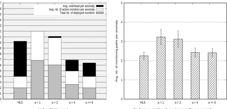
0 1 2 3 4 5 6 7 8 9 10 11 12 13 14 15 16 17 HLS α = 1 α = 2 α = 4 α >= 6 Total nb. of deployed monitors Avg. nb. of active monitors per anomaly Avg. overhead per anomaly

(a) Localization cost

0 1 2 3 4 5 HLS α = 1 α = 2 α = 4 α >= 6

Avg. nb. of monitoring paths per anomaly

(b) Average number of monitoring paths per anomaly

Fig. 3:Numerical results for TOP(8, 18). In each of the two sub-graphs, the first histogram to the left presents results for solutions computed using the hybrid localization scheme (HLS), and the other histograms present results for the solutions computed using our anomaly localization ILP with different values of α.

takes as input any detection solution that covers all links of the network. Detection solutions are computed using the anomaly detection scheme proposed in [11]. For our anomaly localization ILP, we set Cn = Ce= 1,∀n ∈ N and ∀e ∈ E.

We set the weight associated to the probe cost β = 1, and we vary the weight associated to the monitor cost α∈ [1, 2, 4, 6[.

B. Simulation Results

We define three metrics for the comparison. The first metric is the time of computing the localization solution, i.e. monitors that are to be activated and paths that are to be monitored when an anomaly is detected. This metric reflects the speed of the localization scheme. The better is to avoid online computations, i.e. computations done upon detecting an anomaly, in order to shorten the localization delay. TABLE III: Average ILP Computation Time (seconds) for TOP(8, 18)

Hybrid scheme Our scheme Offline Computation Time 64.16 6.67 Online Computation Time 25.7 10−3 0

Table III depicts the online computation time and the offline computation time for the hybrid localization scheme and for our localization scheme. Intuitively, as shown in the table, the online computation time is zero for our localization scheme. This is because we compute full localization solutions for all potential anomalies offline. In contradiction, the hybrid scheme leaves the selection of monitoring paths upon detecting an anomaly, thereby achieving a non-negligible online computa-tion time. This time can be relatively high for large topologies

where the number of candidate monitoring paths is large. For the offline computation time, the table shows that our scheme is about 10 times faster than the hybrid scheme, although, it computes full localization solutions for all potential anomalies. We explain this result by the fact that, unlike the hybrid scheme, our scheme does not distinguish between every pair of the network links.

The second metric is the localization cost. Fig. 3a plots the total number of deployed monitors, the average number of active monitors per anomaly, and the average overhead, i.e. the number of links monitored that provide no localization information, per anomaly for the hybrid localization scheme and for our localization scheme with α ∈ [1, 2, 4, 6[. Three conclusions can be drawn from the numerical results. The first is that there is an interplay between the monitor location cost and the probe cost. The different results for the different values of α illustrate this conclusion. Indeed, the larger the value of

α is, the fewer the number of monitors is and the larger the

localization overhead is. For instance, for α = 1, we have localization solutions with zero overhead and 7 monitors, i.e. 7 of the 8 nodes of the network hold monitoring devices. The second is that the existing localization scheme that deploys monitors offline and selects monitoring paths online does not take into consideration this interplay, and therefore, delivers sub-optimal localization solutions. In effect, using the same number of monitors, for α≥ 6, our localization scheme can localize any potential anomaly with about 65% less overhead than the existing localization scheme.

this is the path selection criterion for the existing localization scheme. We do not consider this criterion in our localization scheme for two reasons. The first is that, upon detecting an anomaly, the set of paths that distinguish between the suspect links are monitored simultaneously. Therefore, the minimization of the number of monitoring paths does not reduce the localization delay. The second reason is that this metric is tightly correlated to the number of monitors and the localization overhead. Indeed, if we relax the constraint on the localization overhead, this would allow long monitoring paths that cross a large number of links. Therefore, the number of monitoring paths that can distinguish between the suspect links would decrease. Likewise, if we relax the constraint on the number of monitors, we would deploy more monitors in the network, thus, the monitoring paths would get shorter. Therefore, the number of monitoring paths that can distinguish between the suspect links would increase. Fig. 3b validates these claims. Hereby, we can observe that the larger α is, the more monitoring paths we have. Not surprisingly, for

α≥ 6, our localization scheme monitors only 18% more paths

than the hybrid localization scheme, while deploying the same number of monitors and incurring 65% less overhead.

IX. ROBUSTNESS OF OURANOMALYLOCALIZATION

SCHEMEAGAINSTTOPOLOGYCHANGES

The anomaly localization solution must be updated when-ever the detection solution changes. Howwhen-ever, the detection solution changes in rare cases where a persistent anomaly makes a network link unavailable for a long period of time, or where the network topology is modified voluntary (e.g. add and/or removal of links and/or nodes). Clearly, in the first case, only the anomaly scenario whose set of suspect links contains the anomalous link is affected by the anomaly. After updating the set of detection paths, the affected anomaly scenario is updated and its localization solution is recomputed. Further, voluntary network changes are usually planned in advance, in which case detection and localization updates should be computed offline before changes are made. We conclude based on this discussion that it is of great importance to provide a fast heuristic for computing localization solutions in order to ensure fast recovery of the localization process in case of persistent anomalies.

X. CONCLUSION

In this paper, we addressed the problem of localizing single link-level anomalies. Two findings were presented and demonstrated: 1) Not all pairs of the the network links need to be distinguishable for localizing all potential link-level anomalies, 2) All potential anomaly scenarios can be derived offline from any detection solution that covers all the network links. These findings were exploited to develop an anomaly localization scheme that computes full localization solutions offline. In order to achieve a good trade-off between the number and locations of monitoring devices and the quality of monitoring paths, monitor locations and monitoring paths are selected jointly. A novel anomaly localization cost model

was proposed, and our localization scheme was formulated as an ILP. However, it was demonstrated that the problem

is N P-hard. Our scheme was compared with an hybrid

anomaly localization scheme that combines the strengths of two existing schemes. Extensive simulations was conducted on small network topologies. Results show that using the same number of monitoring devices, our schemes incurs 65% less overhead than the hybrid scheme. Our ongoing work is on the design of a scalable, cost-efficient and fast heuristic solution. Furthermore, we are working on extending our scheme to localize multiple link-level anomalies.

APPENDIXA

This section presents the proofs of corollaries 2, 3, 4, 5 and 6.

• Corollary 2: e1∈ S(e2)⇔ S(e1) =S(e2),∀e1, e2∈ E

Proof: e1∈ S(e2)⇔ (according to Theorem 1) there

does not exist any path that crosses either e1 or e2, but

not both⇔ for each p ∈ P, p crosses both e2and e1, or p

neither crosses e1 nor e2⇔ De1+= De2+ and De1−=

De2− ⇔ (according to Theorem 2) S(e1) =S(e2)

• Corollary 4:S(e1)6= S(e2)⇔ S(e1)∩ S(e2) =∅

Proof: We prove the direct implication by

contra-diction. Assume to the contrary thatS(e1)6= S(e2) and

S(e1)∩ S(e2)6= ∅. Let e3 ∈ S(e1)∩ S(e2). According

Corollary 2, S(e3) = S(e1) and S(e3) = S(e2). thus,

S(e1) = S(e2), leading to a contradiction. The indirect

implication is trivially true.

• Corollary 3:∪e_∈ES(e) = ∪_S(i)∈dSS(i) = E

Proof: According to Theorem 2, e ∈ S(e), ∀e ∈ E. Thus, ∪e_∈ES(e) = E. Obviously, ∪e_∈ES(e) =

∪S(i)∈dSS(i).

• Corollary 5: X

S(i)∈dS

| S(i) | = | E |

Proof: According to Corollary 4, | ∪_S(i)∈dSS(i) |=|

E |, and according to Corollary 2, ∩_S(i)∈dSS(i) = ∅. Thus, X

S(i)∈dS

| S(i) | = | E |.

• Corollary 6: dP airs = AllP airs - X

S(i),S(j)∈dS:i<j

| S(i) | ∗ | S(j) |

Proof: According to Corollary 1, only links that

belong to same set of suspect links need to be distinguish-able pairwise. Therefore, the set of link pairs that are to be distinguished can be expressed as{{(ei, ej); ei, ej ∈ E}

-{(ei, ej);S(ei)6= S(ej)}}. We conclude that dP airs = AllP airs - X

S(i),S(j)∈dS:i<j

| S(i) | ∗ | S(j) |. Clearly, the number of pair of links that need to be distinguishable equals the number of all link pairs of the network if and only if the number of distinct sets of suspect links equals 1, i.e. the number of detection paths equals 1.

APPENDIXB

Proof: Paths in P0 can be divided into three subsets of paths.

• P1: paths that cross either e1 or e2, but not both.

• P2: paths that cross both e1 and e2.

• P3: paths that neither cross e1 nor e2.

On the one hand, we have

∀p ∈ P2, δpe1= 0 and δpe2 = 0.

Thus,∀p ∈ P2, (δpe1+ δpe2− 2δpe1δpe2) = 0.

Contributing to ∑_p∈P

2(δpe1+ δpe2− 2δpe1δpe2) > 0.

On the other hand, we have∀p ∈ P3, δpe1= 1 and δpe2 = 1.

Thus,∀p ∈ P3, (δpe1+ δpe2− 2δpe1δpe2) = 0. Contributing to ∑_p∈P 3(δpe1+ δpe2− 2δpe1δpe2) = 0. Subsequently, ∑_p∈P0(δpe1 + δpe2 − 2δpe1δpe2) = ∑ p_∈P1(δpe1+ δpe2− 2δpe1δpe2).

Now, we have ∀p ∈ P1 δpe1+ δpe2= 1 and δpe1δpe2 = 0.

Thus, δpe1+ δpe2− 2δpe1δpe2 = 1. Therefore,∑_p∈P 1(δpe1+ δpe2− 2δpe1δpe2) = Cardinal(P1). We conclude that ∑_p∈P0(δpe1 + δpe2 − 2δpe1δpe2) = Cardinal(P1). REFERENCES

[1] A. Adams, T. Bu, R. Caceres, N. Duffield, T. Friedman, J. Horowitz, F.L. Presti, S.B. Moon, V. Paxson, and D. Towsley, The Use of End-to-End Multicast Measurements for Characterizing Internal Network Behavior, IEEE Communications, 2000.

[2] V.N. Padamanabahn,L. Qiu, and H.J. Wang Server-Based Inference of Internet Performance, IEEE INFOCOM, 2003.

[3] N. Duffield, Network Tomography of Binary Network Performance Char-acteristics, IEEE Transactions on Information Theory, vol. 52, pp. 5373-5388, 2006.

[4] A. Dhamdhere, R. Teixeira, C. Dovrolis, and C. Diot NetDiagnoser: Troubleshooting Network Unreachabilities Using End-to-End Probes and Routing Data, ACM CoNEXT, 2006.

[5] Y. Bejerano, and R. Rastogi, Robust Monitoring of Link Delays and Faults in IP Networks, IEEE/ACM Transactions on Networking, 2006. [6] Y. Zaho, Z. Zhu, Y. Chen, D. Pei, and J. Wang, Towards Efficient

Large-Scale VPN Monitoring and Diagnosis under Operational Constraints, IEEE INFOCOM, 2009.

[7] S Argawal, K.V.M. Naidu, and R. Rastogi, Diagnosing Link-Level Anoma-lies Using Passive Probes, IEEE INFOCOM, 2007.

[8] P. Barford, N. Duffield, A. Ron, and J. Sommers, Network Performance Anomaly Detection and Localization, IEEE INFOCOM, 2009. [9] H.X. Nguyen, R. Teixeira, P. Thiran, and C. Diot, Minimizing Probing

Cost for Detecting Interface Failures: Algorithms and Scalability Analy-sis, IEEE INFOCOM, 2009.

[10] L. Cheng, X. Qiu, L. Meng, Y. Qiao, and R. Boutaba, Efficient Active Probing for Fault Diagnosis in Large Scale and Noisy Networks, IEEE INFOCOM, 2010.

[11] E. Salhi, S. Lahoud, and B. Cousin, Joint Optimization of Monitor Location and Network Anomaly Detection, IEEE LCN, 2010.

[12] E. Salhi, S. Lahoud, and B. Cousin, Heuristics for Joint Optimization of Monitor Location and Network Anomaly Detection, IEEE ICC, 2011. [13] F. Chudak, and D. Chmyos, Improved Approximation Algorithms for the Uncapacitated Facility Location Problem, ACM SIAM Journal on Computing, vol. 33.1, pp. 1-25, 2004.

[14] BRITE, [Online]. Available: http://www.cs.bu.edu/brite/. Last accessed February, 2012.

[15] Cplex, [Online]. Available: http://www.ilog.com/products/cplex. Last accessed February, 2012.