HAL Id: hal-02947228
https://hal.archives-ouvertes.fr/hal-02947228
Submitted on 23 Sep 2020
HAL is a multi-disciplinary open access
archive for the deposit and dissemination of
sci-entific research documents, whether they are
pub-lished or not. The documents may come from
teaching and research institutions in France or
abroad, or from public or private research centers.
L’archive ouverte pluridisciplinaire HAL, est
destinée au dépôt et à la diffusion de documents
scientifiques de niveau recherche, publiés ou non,
émanant des établissements d’enseignement et de
recherche français ou étrangers, des laboratoires
publics ou privés.
Operation Modes and Self-motions of a 2-RUU Parallel
Manipulator
Latifah Nurahmi, Stéphane Caro, Philippe Wenger
To cite this version:
Latifah Nurahmi, Stéphane Caro, Philippe Wenger. Operation Modes and Self-motions of a 2-RUU
Parallel Manipulator. The 3rd IFToMM Symposium on Mechanism Design for Robotics, Jun 2015,
Aalborg, Denmark. �hal-02947228�
Operation Modes and Self-motions of a 2-RUU
Parallel Manipulator
Latifah Nurahmi, St´ephane Caro†, Philippe Wenger
Institut de Recherche en Communications et Cybern´etique de Nantes, France, e-mails:{latifah.nurahmi,stephane.caro,philippe.wenger}@irccyn.ec-nantes.fr
Abstract. This paper deals with the characterization of the operation modes of the 2-RUU parallel
manipulator with an algebraic approach, namely the Study kinematic mapping of the Euclidean group SE(3). The manipulator is described by a set of eight constraint equations and the primary decomposition reveals that the mechanism has three operation modes. The singularity conditions are obtained by deriving the determinant of the Jacobian matrix of the constraint equations with respect to the Study parameters. It is shown that there exist singular configurations in which the 2-RUU manipulator may switch from one operation mode to another operation mode. All the singular configurations are mapped onto the joint space and are geometrically interpreted. Finally, the mechanism may switch from the 1st Sch¨onflies mode to the 2nd Sch¨onflies mode through the additional mode that contains self-motions.
Key words: Sch¨onflies motion, operation mode, Study parameters, 2-RUU manipulator,
self-motion.
1 Introduction
Lower-mobility parallel manipulators are suitable for wide range of applications that require fewer than six degree-of-freedom end-effector motion (6-dof ), for ex-ample Sch¨onflies Motion Generators (SMGs). The SMGs are manipulators which can exhibit three independent translations and one pure rotation about an axis of fixed direction, for example the 2-RUU parallel manipulator. This mechanism is composed of two RUU limbs in which two joints are actuated in each limb.
By using an algebraic description of the manipulator and the Study parametriza-tion based on [3], [5], the operaparametriza-tion modes of the 2-RUU manipulator are discussed in more details in this paper. The constraint equations are initially derived. Then the primary decomposition is computed over the set of constraint equations to reveal the existence of three operations modes. The singularities are examined by deriving the determinant of the Jacobian matrix of the constraint equations with respect to the Study parameters. It is shown that the mechanism is able to change from one mode to another mode by passing through the configurations that belong to both modes.
† Corresponding author. Email: stephane.caro@irccyn.ec-nantes.fr. Tel: +33 (02) 40 37 69 68
2 Latifah Nurahmi, St´ephane Caro‡, Philippe Wenger
The singularity conditions are mapped onto the joint space. Eventually, the changes of operation modes for the 2-RUU parallel manipulator are illustrated.
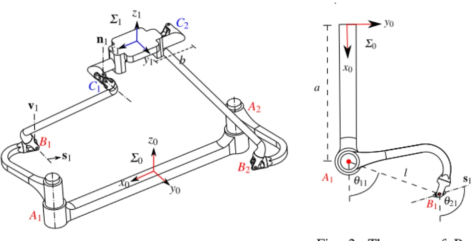
A1 A2 B1 B2 C1 C2 s1 v1 n1 Σ0 Σ1 b x0 y 0 z0 x1 y1 z1
Fig. 1: The 2-RUU parallel manipulator.
Σ0 x0 y0 θ11 θ21 s1 l a A1 B1
Fig. 2: The axes of R-joints from top view.
2 Manipulator architecture
The 2-RUU parallel manipulator shown in Fig.1, is composed of a base, a moving platform, and two identical limbs. Each limb is composed of five revolute joints such that the second and the third ones, as well as the forth and the fifth ones, are built with intersecting and perpendicular axes. Thus they are assimilated to U-joint. The first revolute joint is attached to the base and is actuated. Its rotation angle is defined byθ1i(i= 1,2). The axes of the first, the second, and the fifth joints are
directed along z-axis. The second axis and the fifth axis are denoted by vi and ni (i= 1,2), respectively. The second revolute joint is also actuated and its rotation angle is defined byθ2i(i= 1,2), in Fig. 2.
The axes of the third and the forth joints are parallel. The axis of the third joint is denoted by si(i= 1,2) and it changes instantaneously as a function ofθ2ias shown
in Fig. 2, i.e.: si= [0,cos(θ2i),sin(θ2i),0]T (i= 1,2).
The fixed frameΣ0is located at the center of the base. The first revolute joint of
the i-th limb is located at point Aiwith distance a from the origin of Σ0. The first
U-joint is denoted by point Biwith distance l from point Ai. Link AiBialways moves in a plane normal to vi. Hence the coordinates of points Aiand Biexpressed in the fixed frameΣ0are:
r0 A1 = [1,a,0,0] T r0 B1 = [1,l cos(θ11) + a,l sin(θ11),0] T r0A 2 = [1,−a,0,0] T r0 B2 = [1,l cos(θ12) − a,l sin(θ12),0] T (1)
The moving frameΣ1is located at the center of the moving platform. The moving
of the revolute joint axes is denoted by Ci. The length of the moving platform from the origin ofΣ1to point Ciis defined by b. The length of link BiCiis defined by r. The coordinates of point Ciexpressed in the moving frameΣ1are:
rC1 1 = [1,b,0,0] T r1 C2= [1,−b,0,0] T (2)
3 Constraint equations
In this section, the constraint equations are derived whose solutions illustrate the possible poses of the moving platform (coordinate frame Σ1) with respect toΣ0.
To obtain the coordinates of points Ci and vectors ni expressed inΣ0, the Study
parametrization of a spatial Euclidean transformation matrix M based on [1] is used. The parameters x0,x1,x2,x3,y0,y1,y2,y3, which appear in matrix M, are called Study parameters. They are useful in the representation of a spatial Euclidean dis-placement and they should satisfy [1] x20+ x2
1+ x22+ x236= 0. This condition will be
used in the following computations to simplify the algebraic expressions. First of all, the half-tangent substitutions forθi j (i,j= 1,2) are performed to remove the trigonometric functions: cos(θi j) = 1− t2 i j 1+ t2 i j , sin(θi j) = 2ti j2 1+ t2 i j , i,j= 1,2 (3) where ti j= tan(θi j
2 ). The coordinates of points Ciand vectors niexpressed inΣ0are obtained by: r0C i= M r 1 Ci , n 0 i = M n1i , i= 1,2 (4)
As the coordinates of all points are given in terms of Study parameters and the design parameters, the constraint equations can be obtained by examining the design of the RUU limb. The link connecting points Bi and Ci is coplanar to the vectors vi and n0i. Accordingly, the scalar triple product of vectors (r0Ci− r
0 Bi), vi and n 0 i vanishes, namely: (r0 Ci− r 0 Bi) T .(vi× n 0 i) = 0 , i= 1,2 (5)
After computing the corresponding scalar triple product, and removing the com-mon denominators, the following constraint equations come out:
g1:(at112 − bt112 − lt112 + a − b + l)x0x1+ 2lt11x0x2− (2t112 + 2)x0y0+ 2lt11x3x1+ (−at2 11− bt112 + lt112 − a − b − l)x3x2+ (−2t112 − 2)y3x3= 0 g2:(at122 − bt122 + lt122 + a − b − l)x0x1− 2lt12x0x2+ (2t122 + 2)x0y0− 2lt12x1x3+ (−at2 12− bt122 − lt122 − a − b + l)x2x3+ (2t122 + 2)x3y3= 0 (6) To derive the constraint equations corresponding to the link length r of link BiCi, the distance equation can be formulated as:k(r0
Ci− r
0
Bi)k
2= r2. As a consequence,
4 Latifah Nurahmi, St´ephane Caro‡, Philippe Wenger
g3:(a2t112 − 2abt112 − 2alt112 + b2t112 + 2blt112 + l2t112 − r2t112 + a2− 2ab + 2al + b2−
2bl+ l2− r2)x2
0− 8blt11x0x3+ (4at112 − 4bt112 − 4lt112 + 4a − 4b + 4l)x0y1+...
g4:(a2t122 − 2abt122 + 2alt122 + b2t122 − 2blt122 + l2t122 − r2t122 + a2− 2ab − 2al + b2+
2bl+ l2− r2)x20+ 8blt12x0x3+ (−4at122 + 4bt122 − 4lt122 − 4a + 4b + 4l)x0y1+... (7) To derive the constraint equations corresponding to the actuation of the second joint of each limb, the scalar product of vector(r0
Ci− r
0
Bi) and vector siis expressed
as:(r0
Ci− r
0
Bi)
Ts
i= 0. Hence, the following constraint equations are obtained:
g5:(−at112t212 + bt112t212 + lt112t212 + at112 − at212 − bt112 + bt212 − lt112 + 4lt11t21− lt212+ a− b + l)x2 0− 4bt21(t112 + 1)x0x3− 2(t212 − 1)(t112 + 1)x0y1+ 4t21(t112 + 1)x0y2... g6:(at122t222 − bt122t222 + lt122t222 − at122 + at222 + bt122 − bt222 − lt122 + 4lt12t22− lt222− a+ b + l)x20+ 4bt22(t122 + 1)x0x3− 2(t222 − 1)(t122 + 1)x0y1+ 4t22(t122 + 1)x0y2... (8) For detail expressions of equations g3,g4,g5,g6, the reader may refer to [6]. All solutions have to be within the Study quadric, i.e.: g7: x0y0+ x1y1+ x2y2+ x3y3= 0.
To exclude the exceptional generators (x0= x1= x2= x3= 0), the normalization
equation is added: g8: x20+ x21+ x22+ x23− 1 = 0.
4 Operation modes
The design parameters are assigned as a= 2,b= 1,l= 1,r= 2. The set of eight con-straint equations is written as a polynomial ideal with variables{x0,x1,x2,x3,y0,y1,
y2,y3} over the coefficient ring C[t11,t12,t21,t22], defined as: I = hg1,g2,g3,g4,g5,
g6,g7,g8i. At this point, the following ideal is examined: J = hg1,g2,g7i. The primary decomposition is computed and it turns out that the ideal J is decomposed into three components as:J =T3
i=1Ji, with the results of primary decomposition:
J1=hx0,x3,x1y1+ x2y2i J2=hx1,x2,x0y0+ x3y3i
J3=h(t112t122 + 2t122 + 1)x0x1+ (−t112t12+ t11t122 + t11− t12)x0x2...i (9)
For complete results of the primary decomposition, the reader may refer to [6]. Accordingly, the 2-RUU manipulator under study has three operation modes. The computation of the Hilbert dimension of idealJiwith t11,t12,t21,t22treated as vari-ables shows that: dim(Ji) = 4 (i = 1..3). To complete the analysis, the remaining equations are added by writing:
Ki:Ji∪ hg3,g4,g5,g6,g8i, i= 1..3 (10)
It follows that the 2-RUU manipulator has 4-dof. Each systemKicorresponds to a specific operation mode that will be discussed in the following.
4.1 System
K
1: 1st Sch¨onflies mode
In this operation mode, the moving platform is reversed about an axis parallel to the xy-plane by 180 degrees from the home position [2]. The condition x0= 0,x3= 0,x1y1+ x2y2= 0 are valid for all poses and are substituted into the transformation matrix M, as: M1= 1 0 0 2(x1y0− x2y3) x21− x22 2x1x2 0 2(x1y3+ x2y0) 2x1x2 −x21+ x22 0 −2y2 x1 0 0 −1 (11)
From the transformation matrix it can be seen that the manipulator has 3-dof trans-lational motions, which are parametrized by y0,y2,y3and 1-dof rotational motion, which is parametrized by x1,x2in connection with x
2
1+ x22− 1 = 0 [4].
4.2 System
K
2: 2nd Sch¨onflies mode
In this operation mode, the condition x1= 0,x2= 0,x0y0+ x3y3= 0 are valid for all
poses. The transformation matrix in this operation mode is:
M2= 1 0 0 0 −2(x0y1− x3y2) x20− x23−2x0x30 −2(x0y2+ x3y1) 2x0x3 x20− x2 3 0 −2y3 x0 0 0 1 (12)
From this transformation matrix, it can be seen that the manipulator has 3-dof trans-lational motions, which are parametrized by y1,y2,y3and 1-dof rotational motion, which is parametrized by x0,x3in connection with x
2
0+ x23− 1 = 0 [4].
4.3 System
K
3: Third mode
In this operation mode, the moving platform is no longer parallel to the base. The variables x3,y0,y1can be solved linearly from idealJ3. Accordingly, the 2-RUU parallel manipulator will perform two translational motions, which are parametrized by variables y2,y3and two rotational motions, which are parametrized by variables
x0,x1,x2in connection with normalization equation g8.
Under this operation mode, the joint angles t21 and t22 can be computed from
Eq.(8). It turns out that no matter the value of the first actuated joint (t11,t12) in each limb, these equations vanish for two real solutions, namely (1.) t21= −
1
t22
and (2.)
t21= t22. As a consequence, in this operation mode, the links BiCi (i= 1,2) from both limbs are always parallel to the same plane and the axes si(i= 1,2) from both limbs are always parallel too.
6 Latifah Nurahmi, St´ephane Caro‡, Philippe Wenger
5 Singularity Conditions and Operation Mode Changing
The 2-RUU manipulator reaches a singularity condition when the determinant of its Jacobian matrix vanishes. The Jacobian matrix is the matrix of all first order partial derivatives of the eight constraint equations with respect to the eight Study parame-ters. Since the 2-RUU manipulator has more than one operation mode, the singular configurations can be classified into two different types, i.e. the configurations that belong to a single operation mode and the singularity configurations that belong to more than one operation mode. The common configurations that belong to more than one operation mode allow the 2-RUU manipulator to switch from one mode to another mode. However, the 1st Sch¨onflies mode and the 2nd Sch¨onflies mode do not have configurations in common, since x0,x1,x2,x3can never vanish simul-taneously. It means that the 2-RUU manipulator cannot switch from the Sch¨onflies mode into the reversed Sch¨onflies mode directly.
To change from the 1st Sch¨onflies mode into the 2nd reversed Sch¨onflies mode, the mechanism should pass through the third mode, namely systemK3, as shown
in Fig. 3. There exist some configurations in which the mechanism can change from the 1st Sch¨onflies mode to the third mode and these configurations belongs to both modes. Noticeably, these configurations are also singular configurations since they lie in the intersection of two operation modes.
5.1 1st Sch¨onflies Mode (
K
1)
←→ Third Mode (K
3)
For the 1st Sch¨onflies mode, the determinant of Jacobian matrix S1: det(J1) = 0
(for complete results of det(J1), the reader may refer to [6]) has four factors. The
first factor is y2= 0, when the moving platform is coplanar to the base, the
mecha-nism is always in a singular configuration. The second factor shows the singularity configurations that lie in the intersection withK2. However, this factor is neglected
since systemsK1andK2do not have configurations in common.
The inspection of the third factor yields the singularity configurations that belong to the 1st Sch¨onflies modeK1and the third modeK3. The third factor is added to
the systemK1. Then, all Study parameters are eliminated. The elimination yields
two polynomials of degree eight and degree nine in t11,t12,t21,t22, respectively. The factorization splits both polynomials into four factors as follows:
f1:(t21t22+ 1)(t21− t22)(t12+ t11)(3t112t122 − 2t11t12+ 8t122 + 3) f2:(t21t22+ 1)(t21− t22)(t122 + 1)(3t112t122 − 2t11t12+ 8t122 + 3)
(13)
Polynomials f1,f2vanish simultaneously when: (1.) t21= − 1
t22
and (2.) t21= t22.
It means that when the second link BiCi(i= 1,2) from both limbs are parallel to the same plane and the moving platform is twisted about an axis parallel to the xy-plane by 180 degrees, the 2-RUU manipulator is in the intersection of the 1st Sch¨onflies mode and the third mode.
Eventually, the last factor of the determinant of Jacobian matrix S1: det(J1) = 0
is analysed. This factor is added to the system K1 and all Study parameters are
eliminated. Due to the heavy elimination process, the joint angles are assigned as
t11= 1,t12= 0,t21= −1 and the result of elimination is a univariate polynomial of
degree 12 in t22.
5.2 2nd Sch¨onflies Mode (K
2)
←→ Third Mode (K
3)
For the 2nd Sch¨onflies mode, the determinant of Jacobian matrix S2: det(J2) = 0
(for complete results of det(J2), the reader may refer to [6]) has four factors too.
The first factor is y3= 0 in which the moving platform is coplanar to the base,
hence the mechanism is always in a singular configuration. The second factor gives the condition in which the mechanism is in the intersection of systemsK1andK2.
As explained in Section 5.1, this factor is removed.
The analysis of the third factor yields the singularity configurations that belong to the 2nd Sch¨onflies modeK2and the third modeK3. The third factor is added to
the systemK2. Then all Study parameters are eliminated and yields: f1:(t21t22+ 1)(t21− t22)(t12+ t11)(3t112t122 − 2t11t12+ 8t122 + 3) f2:(t21t22+ 1)(t21− t22)(t122 + 1)(3t112t122 − 2t11t12+ 8t122 + 3)
(14) Notably, the elimination results have the same mathematical expressions as in Eq.(13) and it leads to the same solutions, namely: (1.) t21= −
1
t22
and (2.) t21= t22.
It means that when the second link BiCi(i= 1,2) from both limbs are parallel to the same plane and the moving platform is parallel to the base, the 2-RUU manipulator is in the intersection of the 2nd Sch¨onflies mode and the third mode.
Finally, the last factor of the determinant of Jacobian matrix S2: det(J2) = 0
is analysed. Due to the heavy elimination process, the joint angles are assigned as
t11= 1,t12= 0,t21= −1 and the result of elimination is also a univariate polynomial of degree 12 in t22.
6 Self-motions in System
K
3The determinant of the Jacobian matrix is computed in the systemK3, which
con-sists of five constraint equations over five variables. Hence the 5× 5 Jacobian matrix can be obtained. The determinant of this Jacobian matrix S3: det(J3) = 0 (for
com-plete results of det(J3), the reader may refer to [6]) consists of 10 factors, two of
them are:(t21t22+ 1) and (t21− t22). It can be seen from Section 4.3 that these
fac-tors are the necessary conditions for the manipulator to be in the systemK3, namely
(1.) t21= −
1
t22
and (2.) t21= t22. It means that every configuration in the systemK3
amounts to a self-motion. Furthermore, the image of the transition configurations in the joint space from Eq.(13), is contained in S3: det(J3) = 0. As a consequence,
8 Latifah Nurahmi, St´ephane Caro‡, Philippe Wenger
the transition between systemsK1andK2occurs through the third systemK3that
contains self-motions. These transition configurations are illustrated in Figs. 3a-3e.
7 Conclusions
In this paper, the method of algebraic geometry was applied to characterize the type of operation modes of the 2-RUU parallel manipulator. The set of eight constraint equations are derived and the primary decomposition is computed. It is shown that the 2-RUU parallel manipulator has three operation modes and the interpretation of each operation mode was given. The singularity conditions were computed and represented in the joint space. It turns out that the mechanism is able to switch from the 1st Sch¨onflies mode to the 2nd Sch¨onflies mode or vice versa, by passing through the third mode that contains self-motions.
(a) 2nd Sch¨onflies mode (b) Transition Pose (c) Third mode
(d) Transition Pose (e) 1st Sch¨onflies mode
Fig. 3: Transition from the 2nd Sch¨onflies mode to the 1st Sch¨onflies mode via the third mode.
References
1. Husty, M. L., Pfurner, M., Schr¨ocker, H-P., Brunnthaler, K.: Algebraic Methods in Mechanism Analysis and Synthesis. Robotica, 25(6) pp. 661-675 (2007).
2. Xianwen Kong: Reconfiguration Analysis of a 3-DOF Parallel Mechanism Using Euler Pa-rameter Quaternions and Algebraic Geometry Method. Mechanism and Machine Theory, 74 pp.188-201 (2014).
3. Nurahmi, L., Schadlbauer, J., Caro, Stephane., Husty, M., Wenger, P.: Kinematic Analysis of the 3-RPS Cube Parallel Manipulator. Journal of Mechanisms and Robotics, 7(1) pp. 011008-1011008-10 (2015).
4. Schadlbauer, J., Nurahmi, L., Husty, M., Wenger, P. and Caro, S.: Operation Modes in Lower-Mobility Parallel Manipulators, Second Conference on Interdisciplinary Applications of Kine-matics, Lima, Peru, September 9–11, (2013).
5. Schadlbauer, J., Walter, D.R., Husty, M.: The 3-RPS Parallel Manipulator from an Algebraic Viewpoint. Mechanism and Machine Theory, 75 pp.161-176 (2014).