HAL Id: halshs-00131849
https://halshs.archives-ouvertes.fr/halshs-00131849
Submitted on 19 Feb 2007
HAL is a multi-disciplinary open access
archive for the deposit and dissemination of sci-entific research documents, whether they are pub-lished or not. The documents may come from teaching and research institutions in France or abroad, or from public or private research centers.
L’archive ouverte pluridisciplinaire HAL, est destinée au dépôt et à la diffusion de documents scientifiques de niveau recherche, publiés ou non, émanant des établissements d’enseignement et de recherche français ou étrangers, des laboratoires publics ou privés.
Spatial Mobility and Returns to Education:Some
Evidence from a Sample of French Youth
Philippe Lemistre, Nicolas Moreau
To cite this version:
Philippe Lemistre, Nicolas Moreau. Spatial Mobility and Returns to Education:Some Evidence from a Sample of French Youth. 2006. �halshs-00131849�
IZA DP No. 2369
Spatial Mobility and Returns to Education:
Some Evidence from a Sample of French Youth
Philippe LemistreNicolas Moreau
DISCUSSION P
APER SERIES
Forschungsinstitut zur Zukunft der Arbeit Institute for the Study of Labor
Spatial Mobility and Returns to
Education: Some Evidence from a
Sample of French Youth
Philippe Lemistre
Cereq and Lirhe, University of Toulouse 1
Nicolas Moreau
Gremaq, University of Toulouse 1 and IZA Bonn
Discussion Paper No. 2369
October 2006
IZA P.O. Box 7240 53072 Bonn Germany Phone: +49-228-3894-0 Fax: +49-228-3894-180 E-mail: iza@iza.orgAny opinions expressed here are those of the author(s) and not those of the institute. Research disseminated by IZA may include views on policy, but the institute itself takes no institutional policy positions.
The Institute for the Study of Labor (IZA) in Bonn is a local and virtual international research center and a place of communication between science, politics and business. IZA is an independent nonprofit company supported by Deutsche Post World Net. The center is associated with the University of Bonn and offers a stimulating research environment through its research networks, research support, and visitors and doctoral programs. IZA engages in (i) original and internationally competitive research in all fields of labor economics, (ii) development of policy concepts, and (iii) dissemination of research results and concepts to the interested public.
IZA Discussion Papers often represent preliminary work and are circulated to encourage discussion. Citation of such a paper should account for its provisional character. A revised version may be
IZA Discussion Paper No. 2369 October 2006
ABSTRACT
Spatial Mobility and Returns to Education:
Some Evidence from a Sample of French Youth
*The purpose of this article is to reevaluate the returns to geographic mobility and to the level of education, taking into account the interaction between these two variables. We have at our disposal an original French database that permits precise calculation of the distance between the place of education and the location of first employment. We thus capture mobility without
a priori regarding the geographical areas selected, and we use kilometric thresholds to
estimate the returns to spatial mobility. Our results suggest decreasing returns to spatial mobility as the distance covered rises and increasing returns to mobility with higher levels of education. In addition, for all levels of education, including the lowest, returns to geographic mobility prove to be positive, for one threshold at least and several distances.
JEL Classification: J31, J61, I21
Keywords: spatial mobility, returns to schooling, earnings function
Corresponding author:
Nicolas Moreau Gremaq
Université des Sciences Sociales de Toulouse Manufacture des Tabacs
Aile J-J Laffont 21 Allée de Brienne 31000 Toulouse France E-mail: nicolas.moreau@univ-tlse1.fr *
1 Introduction
In this paper, we use an original French data set, the “Generation Survey 98” (Enquête
génération 98), to estimate the returns to education and to geographic mobility for a sample of
young men who left the French educational system in 1998. This mobility concerns the acquisition of a first employment. The mobility in question is between the town in which the youths complete their education and the town in which they obtain their first employment. We look at what factors influence their education level and their spatial mobility and the returns to these decisions.
In the literature, the returns to spatial mobility are often estimated by considering “education” as an exogenous variable even though its endogeneity has been firmly established - see Card (2001) for instance. The goal of this article is to reevaluate the returns to spatial mobility and the returns to education when these variables are assumed endogenous. We use a flexible specification that allows the returns to spatial mobility to depend on the level of education. For this purpose, we have at our disposition a database that allows us to collect precise information, both on the determinants of the level of education and on migration. However, the originality of the data resides especially in calculating the distances covered for each decision of mobility between towns. We can thus characterize mobility without a priori concerning the geographic areas selected by estimating the returns to spatial mobility for different kilometric thresholds.
This method contrasts with studies such as Raphael and Riker (1999) on US data, using a dummy variable for spatial mobility, and Détang-Dessendre, Drapier and Jayet (2004) on French data, that consider work migrations between administrative departments. Also, since
we focus on the first job experience of individuals who all leave the educational system in 1998, we avoid the traditional cohort effect problems and pitfalls related to work experience.1 The results of the paper suggest returns to spatial mobility that increase with the level of education and that depend on the distance covered. It seems that the positive effect of spatial mobility on earnings decreases with distance.
Section 2 exposes the theoretical background. In Section 3, we present the data and the empirical model. In Sections 4, we summarize the empirical findings and discuss some of their implications. Section 5 concludes the text.
2 Economic background: mobility and wages
The introduction of the spatial dimension into the theory of employment prospection (Lippman and McCall, 1976), consists of taking into account the extent of the geographic area prospected (Wolpin, 1987). The individual no longer faces a unique labor market, but a multitude of local labor markets. Broadening the prospection area increases the supply of jobs offered, and thus the probability that one among them will be selected (Pickles and Rogerson, 1983). The choice of changing zones of employment is linked to control over information, generally correlated with the level of education, which is itself determinant of the cost of migration. For the theory of human capital in particular, it is the arbitrage between these costs and the wage advantage associated with migration that leads to migration or not. Prospection takes place if the anticipated wage, less the cost of migration, is superior to the anticipated wage in the initial location (Todaro, 1969).
Two types of mobility costs, direct costs of mobility (transportation, lodging, child care)2 and opportunity costs of mobility (earnings forgone while travelling, searching for job, “psychic
1
See Card and Lemieux (2001) for a clear account of cohort effects. See Knight and Sabot (1981) and Abraham and Medof (1981) for problems related to job experience in earnings functions.
2
The cost of housing is important in the case under study here because we are considering youth who obtain their first job and who may therefore have to leave the lodgings of their parents.
costs”, amenities)3 affect mobility choice. Parts of these costs will be function of the distance of migration (Sjaastad, 1962). In addition, studies that analyze the impact of migration on wages in the human capital framework stem from the hypothesis that an individual who migrates may be intrinsically more motivated to invest in human capital (not only through migration) than others. Therefore, whatever his migration decision, this individual will receive better wages (Greenwood, 1997).
However, the migration does not have necessarily a positive effect on the wages. In fact, individuals could choose to migrate to compensate for their insufficiency in the human capital form. In this case, it is not the “best” who migrate, but the youth of “average value”. The most accomplished among them obtain the best jobs in their own employment area, obliging other youths to migrate to capture more numerous opportunities in other employment areas (Détang-Dessendre, Drapier and Jayet, 2004). Another reason is that migration responds to non-compensating wage differentials (Hunt, 1993). Consequently, if individuals have preferences for certain amenities (for example, climate amenities, warmth versus cold), then equilibrium wages will be lower in regions characterized by more of the amenity. The lower regional wages do not imply lower utility because the lower wages are compensating for the attractive amenity (Hunt and Mueller, 2004).
For example, Falaris (1988), on a sample of young workers two years after exit of the education system, find negative returns for two regions and non significant for two others, whereas many other studies report non significant returns. Détang-Dessendre, Drapier and Jayet (2004), using a sample of youth departing from the French educational system, find positive returns only for those with the highest degrees and non-significant returns for the others. On US data (current population survey, displaced workers files 1986 – 1988 – 1990),
3
Since people are often genuinely reluctant to leave familiar surroundings, family and friends, migration involves a psychic cost (Sjaastad, 1962).
Gabriel and Schmitz (1995) and Raphaël and Riker (1999) (young workers men between 1985 and 1991- SMSA) show positive returns to migration.
A possible explanation of the differences in results is the geographical area retained. Indeed, what is a “migration”? Plainly, the question does not have a clear empirical answer. In this domain, the areas of mobility selected are either the result of administrative divisions, whose logical structure is not necessarily justified from an economic standpoint, or stem from efforts to define homogenous areas according to diverse criteria (economic homogeneity, infrastructure endowment). Examples of the first case would be “regions” and “departments”. An example of the second, for France, would be “Employment zones”.4
Migration is then defined as mobility from one of theses geographic areas to another of the same type. Beyond problems of homogeneity within each spatial division, such conventions pose two types of well-known problems: migrations close to the border and amplitude of the migrations (Hunt and Mueller, 2004). To begin with, individuals situated close to the border of a geographic area are counted as migrants even if they simply cross the borderline, perhaps representing just a short trip from home to work for some of them. Besides, geographic areas with the same nomenclature do not always have the same size and are evidently not all equidistant. Hence, mobility between two small areas can be counted as a migration while mobility within a single large geographic area will not, even though the distance covered in the second case may well be much greater than in the first.
To solve this problem, at least partly, we make no hypothesis about the homogeneity of geographic areas and compensate for the inconveniences linked to the amplitude of mobility by using distances covered. We characterize mobility without a priori concerning the geographic areas selected by estimating the returns to spatial mobility for different kilometric thresholds.
4
It is similar to the Travel-To-Work Area in the United-Kingdom or to the Local Labour System for Italy. Each zone is defined so that the majority of the resident population has a job within its borders and that the firms located there hire the majority of their workforce from within the same area.
3 Data and empirical model
3.1 Sample selection
We have exploited data in the Céreq’s “Generation 98” survey in which 55,000 youths who left the French educational system with an initial education in 1998 are observed over a three-year period. They are representative of the whole generation of those leaving (700,000). The sample retained in this study contains only young men who obtained a first full-time job, which is 24,587 youths. The restriction of the scope of investigation to men with a full-time job is due to the availability of monthly salary data alone, without variables sufficiently detailed to take into account part-time work - while numerous women work part time.
The fact that we have at our disposal a single generation of youth leaving the educational system allows us to avoid several problems encountered in the estimation of the gains functions. The problems linked to the inverse correlation between the duration of schooling and experience in the labor market do not exist here: all individuals in the sample enter the labor market at the same moment (1998).5 Furthermore, cohort effects are limited, a single generation of labor-market entrants being present,6 and these cohort effects are not neutral with respect to the returns to education (Harmon and Walker, 1995, Card and Lemieux, 2001). Lastly, our choice of restricting analysis to starting salaries when first hired is linked to our intention of not making the analysis more complex than need be. If we were to take into account the subsequent job history, the variables that characterize it would probably also be endogenous, which would require a complex, dynamic model.
5
Even if they do not find a work immediately.
6
Youth who left the educational system in 1998 were evidently not all born in the same year. However, dispersion in terms of age rarely exceeds 5 years, and birth cohorts usually concern a minimum of 5 consecutive years.
3.2 Mobility and education levels variables
The distances covered between the towns are calculated “as the crow flies” between the centers of the towns of departure and the towns of arrival. In a pair (x,y) representing the geographic coordinates of a set of points, the distance between point A (departure) and B (arrival) is given by the equation d(A,B)= (xB −xA)²+(yB − yA)². Departure is the place of completion of education (1998) and arrival the place of the first job.
Since mobility near the border and short trips exist, we test several thresholds to account for “relevant” spatial migration: 0 (a change between towns = a mobility), 20 kilometers,7 50 kilometers and 100 kilometers. For each threshold, mobility has a meaning only beyond that threshold. For example, if the threshold is 20 kilometers, a youth who travels 55 km carries out a mobility of 35 km. The decision to migrate in this case is based on a change of towns 20 km apart. For a 50 km threshold, the distance is 5 km; and for a threshold of 100 km, the youth is considered non-mobile. Here we come back to the differences that can exist between partition by region versus division by Employment zones for example.
The variable that characterizes the level of education is the highest level attained and not the number of years of study. Indeed, the latter reflects rather poorly the amount of accumulated human capital as it often corresponds to a period of study superior to the length time necessary to obtain the degree. For instance, for 15 years of study (counted beyond the age of 6), which in theory corresponds to the French Baccalauréat + 2 years, only 50% of youth have reached this level, while 26% have the level of the Baccalauréat, (“Bac” hereafter). The level of the remaining students is still lower. Moreover, less than 30% of youth reach the level of the Bac after 13 years of study. The remaining students have a lower level, even no qualification at all, after retaking numerous academic years.
7
The variable we construct takes on a limited number of values, corresponding to different levels of schooling: without qualification, the first level of professional training,8 the Bac, Bac+1, Bac+2, Bac+3, Bac+4, Bac+5, >Bac+5.
Table (1) exhibits some descriptive statistics of the sample. One individual out of four has completed at least 14 years of study (P25). 10% of them earn at least 1829 euros per month (P90). About 72.4% work in a town different from the one in which they finished their studies. For 50% of them, the distance between the two towns remains limited - less than 20 kilometers (P50).
TABLE (1) HERE
3.3 The empirical model
The complete model is:
log(wage) = b0 + b1y1 + b2y2 + b12(y1y2) + b22(y2)2 + b3y3 + X1b + u (1)
y1 = δ1 + e
W
e 1 (2)
y2 = Wδ2 + e2 if y2 > 0 and P(y2 = 0 | W) = 1 − Φ (Wβ2) otherwise (3)
(y1y2) = Wδ12 + e12 if y1y2 > 0 and P(y1y2 = 0 | W) = 1 − Φ (Wβ12) otherwise (4)
(y2)2 = Wδ22 + e22 if y22 > 0 and P(y22 = 0 | W) = 1 − Φ (Wβ22) otherwise (5)
y3 = 1I (Wδ3 + e3 > 0) (6)
y4 = 1I (Wδ4 + e4 > 0). (7)
The first equation of interest is the structural equation where y1 is the education level and y2
the distance covered between the student’s place of residence at the end of his studies and the site of his first employment. The distance in question is the distance beyond the threshold of mobility (which is equal to 0, 20, 50 or 100 km, depending on the estimation). We call this measure “spatial mobility” in what follows. Additionally, y3 is a dummy variable for living in
the Paris region. All else being equal, Paris/province partition clearly determines the most
8
significant differences of salary in France. Finally, X1 is a vector that includes socioeconomic
variables.
This specification allows flexible responses of wage to spatial mobility. In addition, the interaction term (y1y2) allows returns from migration to differ according to the level of
education. Ideally, we should also include a quadratic term in years of schooling to account for a possible non-monotonic relationship between education and wages. However, education and its square are nearly collinear in our data.
As discussed in the literature, earnings equations suffer from heterogeneity and selection bias. Heterogeneity is usually associated with individual ability and motivation that are likely correlated with education and spatial migration. Endogeneity of living in the Paris region is another potential problem. Finally, we observe the wage rate only for those who choose to work which may induce a selectivity bias. Therefore, we have chosen to instrument the education level (equation (2)), the spatial migration (equation (3)), its interaction with education level (equation (4)), its square (equation (5)) and the Paris region (equation (6)). Equation (7) is the selection equation on full-time jobs. We allow arbitrary correlation among
u, e1, e2, e12, e22, e3 and e4. The matrix W includes the exogenous regressors X1 as well as the
matrix X2 of excluded instruments. It is described below.
We estimate years of schooling with a Poisson regression model (Poisson QMLE) since they only take on non-negative integer values.9 Spatial mobility, its square and its interaction with education are estimated with a two-part model. It is partly continuous with many observations at 0. Unlike the standard Tobit model, this specification allows the initial decision of y2 > 0
versus y2 = 0 to be separate from the decision of how much y2 given that y2 > 0. Finally, we
use binary response models for the Paris region and the selection equation.
9
We also estimate the level of education with a negative binomial model (QMLE). The results are similar. See Table A1, Appendix A.
To estimate our model, we use a two-step procedure. First, the six reduced forms are estimated separately; then the wage equation is estimated using OLS on
log(wage) = b0 + b1y1 + b2y2 + b12(y1y2) + b22(y2)2 + b3y3 + X1b + (8)
γ1vˆ1 + γ2vˆ2 + γ12vˆ12 + γ22vˆ22 + γ3vˆ3 + γ4vˆ4 + ε,
where ε is a random term that represents the unobserved heterogeneity. The are the residuals from reduced forms to control for the potential endogeneity of years of schooling (
vˆ
vˆ1), distance to work (vˆ2, a generalized residual from a two-part model), the interaction
between distance to work and education (vˆ12, another generalized residual from a two-part
model), the square of distance to work (vˆ22, a last generalized residual from a two-part
model), the Paris region (vˆ3, an inverse Mill’s ratio) and selection (vˆ4, another inverse Mill’s
ratio). It also provides a direct test of exogeneity by means of the t−statistics of the estimates of γ; see Blundell, Duncan and Meghir (1998) for an application of this control function approach. The asymptotic covariance matrix of the second step estimator is computed using the results of Newey (1984) and Newey and McFadden (1994) to take into account that we are conditioning on generated regressors (that is, vˆ1, vˆ2, vˆ12, vˆ22, vˆ3 and vˆ4). It is robust to
heteroskedasticity of unknown form.
At this stage, the selection of the instruments that appear in the auxiliary regressions (2) to (7) requires some discussion. In the literature, differences of education levels are often attributable to borrowing constraints. Two types of schooling costs affect the borrowing constraints: opportunity costs of schooling (the value of earnings forgone while in school) and direct costs of schooling (monetary cost of tuition, books, transportation, and board and room if necessary). 10
10
See Card (1999, 2001) for a survey on effects of family background. Card (1995), then Cameron and Taber (2004) capture the borrowing constraints also by a proxy for the proximity of the learning establishment. We do not have this variable in our data base.
Carneiro and Heckman (2002) distinguish between two types of borrowing constraints, one in the short term and one in the long term. The first concerns financing capacity at a given moment (that is, at the date of the survey) and plays a limited role. The second, the long-term constraint that weighs on the entire duration of schooling (and perhaps at the entry on the labour market), reflects notably family background. In this perspective, the differences in education levels for youth with identical, ex-ante aptitudes are primarily attributed to
differences in family background and family income.Thus for many studies, family background and family income are likely to influence the level of education.
Mobility is also not independent of family background and income which influences the costs of migration (Détang-Dessendre, Drapier and Jayet, 2004). In addition, migration behaviour remains highly associated with territorial characteristics. For example, information circulates more easily and in greater quantity in urban markets than in rural markets, which reduces the cost of information research. Spatial mobility therefore remains particularly constrained by the characteristics of the territory. Another reason for taking into account the characteristics of territory is the existence of amenities that are likely to compensate for unfavourable salary differences by increasing the opportunity cost of migration (Gabriel and Schmitz, 1995). Along these lines, with respect to family background and income variables, we include as instruments a set of variables that represent the youths’ social origin by indicators of their parents’ professions and their nationalities. More innovative is that we account for the parents’ occupational status at the time when the youth leaves the education system in 1998 (father or mother unemployed, salaried, retired, etc.). With respect to territorial characteristics, we include as instruments a set of variables that characterize the place of completion of education: area of studies (for taking into account amenities, notably), surface and density of population of the Employment Zone of studies, lives in a rural area at the end of schooling. Our intuition is that all these variables have an impact on the various endogenous variables and on the selection equation.
However, some of these instruments are probably important determinants of wages. As a matter of fact, some family background factors (father’s profession: farmer, technician, unknown and mother’s profession: farmer, clerk, inactive) appear to be significant determinants of wages in our estimation. Some regional variables (population density of the Employment Zone of studies, whether he lives in a rural area at the end of schooling) are also statistically significant in the wage equation. Therefore, we decide to control for these variables in the wage equation.
If we allow the regions of studies and the father’s nationality to appear in the wage equation, they are statistically significant but the estimates of the parameters related to spatial migration become imprecise. We thus maintain these exclusion restrictions. It is made primarily for want of decent instruments.
All in all, there are 15 included instruments (a constant, three dummies for the father’s profession, three dummies for the mother’s profession, two regional variables and six generalised residuals) and 24 excluded instruments from the wage equation (region to be educated (7 dummies), surface of the Employment Zone of studies, parents’ origin (4 dummies), parents’ occupational status(5 dummies), Father's profession (3 dummies), Mother’s profession (4 dummies)). Let us now turn to the results.
4
Results
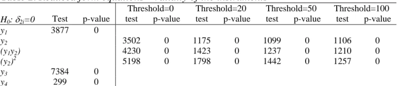
Before we present any further results we report in Table (2) statistics that test the validity of the excluded instruments in all the auxiliary regressions and for all thresholds. Under the null hypothesis, none of them is significant. The corresponding p-values are close to zero, indicating that it is clearly rejected. These results provide evidence that the instruments are significant for all the endogenous variables. The estimates of the auxiliary regressions are shown in Appendix A. To save space, for equations (4) and (5), we only report the results at the 20 km threshold.
TABLE (2) HERE
4.1 Auxiliary regressions: education level and mobility
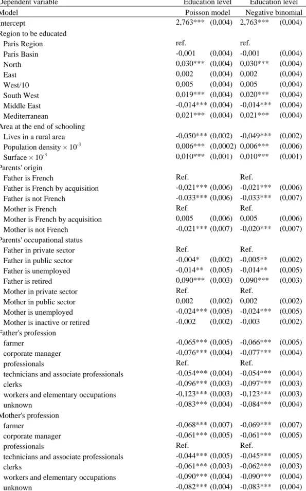
Table A1 in Appendix A displays the results of the estimation of the level of schooling with the Poisson model. Public authorities have attempted to improve the distribution of the offer of education over the French territory.11 Obviously, the regional disparities remain. Indicators of schooling location are in fact often significant. Paradoxically, it seems that discrepancies sometimes are favorable in comparison to the reference, the Paris region. Nevertheless, this is a ceteris paribus analysis. Among the explanatory variables figure also the population density
and the rural nature of the school setting, which influence respectively positively and negatively the level of schooling. On the contrary, the Parisian region’s population density is at least 5 times greater than that of other regions and manifestly is not situated in a rural zone. Having a foreign father or mother lowers the level of studies attained. The great majority of foreigners are immigrants with low qualifications, and that can be reflected in children’s difficulties to adapt to the educational system (language and initial level problems, parents’ low education level) and in the borrowing constraints as well.
If either the father or the mother is unemployed at the time the child leaves the educational system, the latter will tend to do shorter studies. It is clear that the short-term borrowing constraints weigh heavily here since the child cannot compensate for his parents’ reduced income by a loan. Such a situation is not surprising in France where parents must very often guarantee any loan to children, whatever their scholastic performance may be. This result contrasts with the findings of Shea (2000) for the United States, which suggest that changes in
11
First, for professional schooling, ever since the legislation on decentralization during the 1980s, regional administrations have much greater power and autonomy, at least in the choice of where to set up new establishments. At the university level, the “University 2000” program put into place during the 1990s, had as its objective to increase the supply of university education while distributing it over wider territory. As a result, the cohort of youths that entered the labor market in 1998 is one of the most numerous, holding the most university degrees of the past two decades. The rate of youth leaving the university possessing a degree rose by five percentage points between 1992 and 1998, increasing from 33% to 38% (Giret and Lemistre, 2004).
parents’ income due to bad luck (job loss notably) have a negligible impact on children’s human capital for most families.
If one considers, as do Cameron and Taber (2004), that the significance of parents’ qualification level indicates an influence of the long term borrowing constraints, then these latter are strong in France. The variables are all significant. The parents’ professions have the effects observed in numerous studies: the more qualified the father or the mother, the higher the children’s educational attainment.
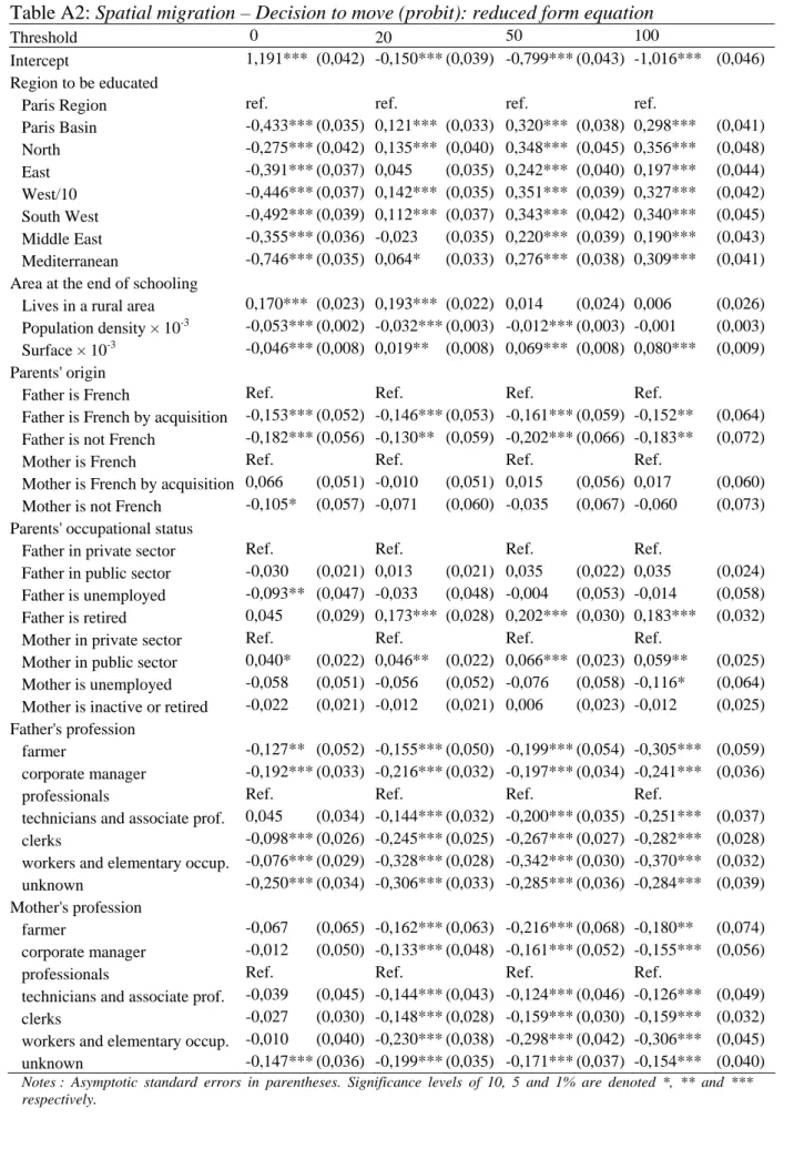
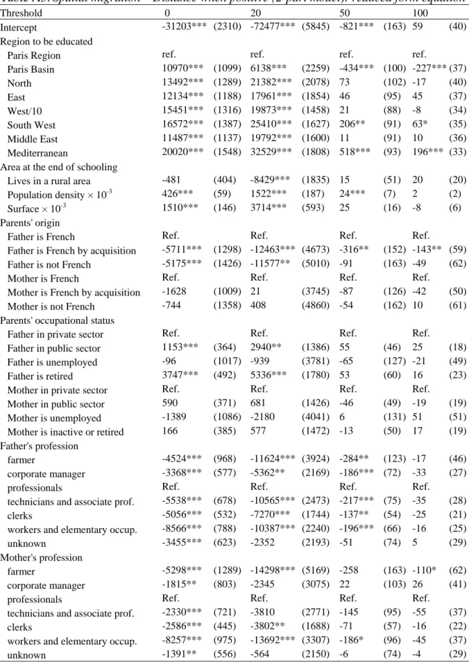
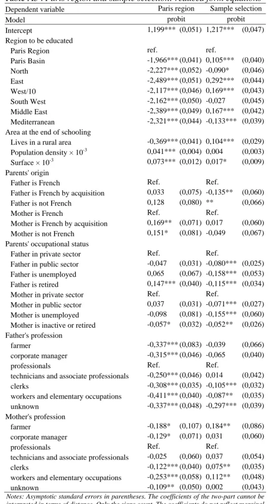
We present the results of the two-part model estimations of equation (3) in Appendix A (Tables A2 and A3) for the different thresholds. When we take into account short-distance migrations (threshold=0), the probability of migration increases for those studying in the Paris region. This result simply reflects the importance of commuting from home to work in the Paris region. A youth who studies in the south of Paris and who finds a first job in the north of Paris is considered mobile for the 0 threshold. Conversely, the probability of migration is lower for those studying in the Paris region for threshold 20 and above.
The effect of the region of education on the distance covered also differs considerably, depending on the threshold selected. However, whatever the threshold chosen, it is when the student originates from the Mediterranean region that the distance covered is the greatest, all else being equal. Many of them find employment in the Paris region, and in general, the coefficients attached to the region of education in the distance equation reflect the remoteness from the Paris region, which is the most important labor market in France.
The fact of residing in a rural area while studying leads to more migration than urban residence, but that geographic situation leads to migrations of lesser amplitude. Inversely, the greater the population density of the Employment zone, the less probable is the migration. The probability of finding employment in a high-density Employment zone is in fact greater. The effects of variables characterizing the parents’ professions while studying are similar to those found for the level of studies. Concerning the parents’ occupational status, their
respective coefficients are not often significant for the probability of migrating or for the distance covered. Next we discuss the wage equation results.
4.2 Wage equation
The results for the estimation of the wage equation at the different thresholds of mobility are presented in Table (3).
TABLE (3) HERE
The coefficient of the residual of the level of studies (vˆ1) is significantly different from 0. The
exogeneity of the level of studies is therefore rejected. The coefficient of the residual (vˆ3) is
also statistically different from 0, which indicates that living in the Paris region in endogenous. We see that living in the Paris region has a positive effect on wages. It mainly reflects the higher standard of living in the Paris area.
Also, there is evidence of selection bias. On the other hand, the residuals corresponding to the distance variables do not have an impact at conventional levels. This comes from the strong correlation between these residuals, leading to large estimated standard errors. However, a joint test leads us to reject the null hypothesis H0: γ 2= γ 12= γ 22=0 at conventional levels,
whatever the estimation. This result provides evidence that the distance covered is endogenous to the earnings function.
We observe that the level of studies, which does not take into account the number of non-validated years of study, has high returns. However, we do not have at our disposal variables characterizing intrinsic individual aptitudes. Several studies have shown that taking into account such variables limits the augmentation of returns to schooling when the education level is instrumented (Eckstein and Wolpin, 1999, Heckman and Carneiro, 2002). It is therefore probable that the returns to schooling are overestimated here. Note too that the returns to schooling increases with the distance covered - the coefficient of (y1y2) being
As for the effect of migration on the salary, we see that the coefficients are positive for the interaction term (y1y2) between the level of studies and the distance covered on the one hand,
and negative for both the distance term ( ) and the quadratic term ( ) on the other hand.
Consequently, the returns to spatial mobility increase with the level of studies but diminish with the distance covered.
2
y y22
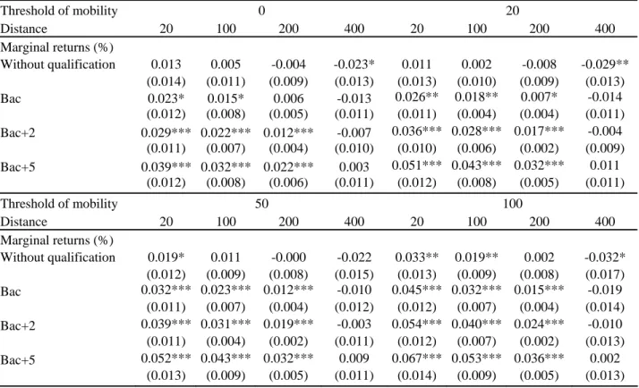
TABLE (4) HERE
Table (4) presents marginal returns to spatial migration. We calculate the marginal returns for each of four levels of education: the lowest (without qualification), then the Bac, Bac+2, and Bac+5, and four distances: 20, 100, 200 and 400 kilometers. For example, at the 20 km threshold, for a distance covered of 100 km and for a youth with an education level of Bac+5, the marginal returns to spatial mobility are 0.043%. At the distance thresholds of 0 and 20 km, the returns are not statistically different from 0 for individuals without qualification, except for long distances for which the returns are negative. Still for individuals without qualification, returns are positive for short distances at the 50 and 100 km thresholds. For higher levels of schooling, spatial returns to migration are positive except for long distances for which the returns are non significant.
While the marginal returns are weak, it is important to keep in mind that they apply to an increase in distance of only one kilometer. The returns to the whole distance are of course greater. They are presented in Table (5) for three distances and four education levels. Other covariates are at the sample median. For a youth with the Bac, at the mobility threshold of 20 km for example, migrating 20 km increases the salary by 1.3% in comparison to the salary of a youth who does not migrate. For a distance covered of 100 km, the salary increase is 3.2%. It is 6.2% for migration distance of 200 km. For a youth with the Bac+5 level, these increases are 1.8%, 8.9% and 17.5% respectively.
A threshold effect manifestly exists. Let us consider a youth who moves by 120 km for example. At the threshold of 20 km, the total return from the kilometers covered (100 km beyond the limit) is 8.9% for a Bac+5 education level. At mobility threshold of 100 km, this return is only 1.5% for the 20 km distance covered beyond the threshold. Our results suggest that choosing a geographic area of great size may lead to an underestimation of returns to the total distance of the migration.
Whatever the level of education, the total returns to distance covered appear positive and statistically significant. In other words, taking into account the distances leads us to nuance the results of Détang-Dessendre, Drapier and Jayet (2004) on French data, who concluded that positive returns to geographic mobility existed exclusively for the highest levels of education.
7 Conclusion
Taking into account distances covered and interactions between the level of education and the first geographical migration leads to several original conclusions.
We have captured spatial mobility without a priori regarding geographical areas selected and
used different kilometric thresholds to characterize this migration. It appears that returns to spatial mobility depend on the threshold selected. The total returns are in general weaker at high thresholds.
Also, taking into account the distance covered between the dwelling place at the end of studies and the site of the first employment widens the range of what returns to spatial mobility can be. Most earlier research in fact makes use of a simple indicator to measure returns from migration. Our results suggest decreasing marginal returns to spatial mobility with distance covered that increases with the level of education. This result is not in contradiction with the theory of employment prospection, or with the hypothesis of a link between the level of human capital and the propensity to migrate.
Finally, we find positive marginal returns to spatial migration for at least one threshold and for several distances, whatever the level of education.
Further investigations should evidently complement this study, focusing in particular on migrations during careers on the labor market. This study is limited to the first migration on departure from the educational system.
References
Abraham K.G. and J.L. Medoff, 1981. Are Those Paid More Really More Productive? The Case of Experience Journal of Human Resources 16, 186-216.
Blundell R., A. Duncan and C. Meghir, 1998. Estimating Labor Supply Responses Using Tax Reforms Econometrica 66, 827-61.
Cameron S. and C. Taber, 2004. Estimation of Educational Borrowing Constraints Using Returns to Schooling Journal of Political Economy 112, 132-182.
Card D., 2001. Estimating the Return to Schooling: Progress on Some Persistent Econometric Problems Econometrica 69, 1127-1160.
Card D., 1999. The causal Effect of Education on Earnings. In: O. Ashenfelter and D. Card (Eds), Handbook of Labor Economics, vol. 3a, North-Holland, Amsterdam, pp.1801-1864.
Card, D., 1995. Using geographic variation in college proximity to estimate the return to schooling, Aspects of labour market behaviour: essays in honour of John Vanderkamp,
University of Toronto Press, Toronto, pp.201-222.
Card D. and T. Lemieux, 2001. Education, Earnings, and the Canadian G. I. Bill Canadian
Journal of Economics 34, 313-344.
Carneiro P. and J.-J Heckman, 2002. The Evidence on Credit Constraints in Post-secondary Schooling Economic Journal 112, 705-734.
Détang-Dessendre C., C. Drapier and H. Jayet, 2004. The Impact of Migration on Wages: Empirical Evidence from French Youth Journal of Regional Science 44, 661-691.
Eckstein Z. And K. Wolpin, 1999. Why youth drop out of high school : the impact of preferences, opportunities, and abilities Econometrica 67, 1295-1340.
Falaris M., 1988. Migration and wage of young men Journal of Human Resources 23,
514-534.
Gabriel, P.E. and S. Schmitz, 1995. Favorable Self-Selection and the Internal Migration of Young White Males in the United States Journal of Human Resources 30, 460-471.
Giret J-F and P. Lemistre, 2004. Declassement of the young people : towards a change of the value of diplomas?, in Special Issue: “Economics of Education and Human Resources”,
Brussels Economic Review 43, 483-504.
Greenwood M.J., 1997. Internal Migration in Developed Countries. In: M. Rosenzweig and O. Stark (Eds), Handbook of Population and Family Economics, Vol. 1B, Elsevier Science,
Harmon C. and I. Walker, 1995. Estimates of the economic return to schooling for the United Kingdom American Economic Review 85, 1278-1286.
Hunt G. And R.E. Mueller, 2004. North American Migration: Returns to Skill, Border Effects, and Mobility Costs Review of Economics and Statistics 86, 988-1007.
Hunt G., 1993. Equilibrium and Disequilibrium in Migration Modelling Regional Studies 27,
341-349.
Knight J. B. and R.H. Sabot, 1981. The Returns to Education: Increasing with Experience or Decreasing with Expansion? Oxford Bulletin of Economics and Statistics 43, 51-71.
Lippman S.A. and J.J McCall, 1976. The Economics of Job Search: a Survey Economic Inquiry 14, 347-368.
Long L., 1988. Migration and Residential Mobility in the United States. Russell Sage Foundation, New-York.
McFadden D. and W. K. Newey, 1994. Large Sample Estimation and Hypothesis Testing. In: R. F. Engle and D.L. McFadden (Eds.), Handbook of econometrics, vol. 4, Elsevier Science
B.V., pp. 2111-2245.
Mac Neal R.B., 1997. Are students being pulled out of high school? The effect of adolescent employment on dropping out Sociology of Education 70, 206-220.
Nakosteen R.A. and M.A. Zimmer, 1982. The Effects on Earnings of Interregional and Interindustry Migration Journal of Regional Science 22, 325-341.
Newey W.K., 1984. A Method of Moments Interpretation of Sequential Estimators
Economics Letters 14, 201-206.
Pickles A. and P. Rogerson, 1983. Wage Distributions and Spatial Preferences in Competitive Job Search and Migration Regional Studies 28, 131-142.
Raphaël S. and D.A Riker, 1999. Geographic Mobility, Race, and Wage Differentials Journal of Urban Economics 45, 17-46.
Shea J., 2000. Does Parents' Money Matter? Journal of Public Economics 77, 155-184.
Sjaastad A. L., 1962. The Costs and Returns of Human Migration Journal of Political Economy 70, 80-93.
Todaro M., 1969. A Model of Labour Migration and Urban Unemployment in LCDs
American Economic Review 59, 138-148.
Wolpin K., 1987. Estimating a Structural Search Model: TheTransition from School to Work
Table 1:Descriptive Statistics of the Sample Live in Paris region 17.5% Live in Couple 26.2%
Migrants 72.4%
P10 P25 P50 P75 P90
Spatial Migration when >0 (in kms) 5 9 20 87 359 Education Level 12 12 14 15 18
Age 18 19 21 23 26
Monthly Wage (in euros) 809 915 1067 1296 1829
Table 2: Reduced form equations - Validity of the instruments -
Threshold=0 Threshold=20 Threshold=50 Threshold=100 H0: δ2i=0 Test p-value test p-value test p-value test p-value test p-value
y1 3877 0 y2 3502 0 1175 0 1099 0 1106 0 (y1y2) 4230 0 1423 0 1237 0 1210 0 (y2)2 5198 0 1798 0 1442 0 1257 0 y3 7384 0 y4 299 0
Notes: δ2i is the vector of parameters corresponding to the excluded instruments X2 in equation i, for i=2,3,4,5,6
and 7. LR tests are used for spatial migration and its related variables, the Paris region and participation. A score statistic is used for years of schooling.
Table 3: Log wage equation
Threshold of mobility 0 20 50 100 Intercept 5,808*** 5,837*** 5,827*** 5,826*** (0,034) (0,034) (0,032) (0,031) y1 0,090*** 0,088*** 0,089*** 0,089*** (0,002) (0,002) (0,002) (0,002) y2 × 10-2 -0,019 -0,038 -0,018 -0,007 (0,026) (0,027) (0,023) (0,025) (y1y2) × 10-3 0,033** 0,051*** 0,040*** 0,043*** (0,015) (0,017) (0,015) (0,016) (y2)2 × 10⁻⁵ -0,047* -0,053** -0,055* -0,085** (0,026) (0,026) (0,029) (0,033) y3 0,070*** 0,071*** 0,073*** 0,073*** (0,010) (0,009) (0,009) (0,009) Lives in a rural area at the end of schooling -0,017*** -0,017*** -0,018*** -0,018***
(0,005) (0,005) (0,005) (0,005) Place of studies, population density × 10-3 0,005*** 0,006*** 0,005*** 0,005***
(0,001) (0,001) (0,001) (0,001) Mother is inactive or retired 0,013*** 0,013*** 0,013*** 0,013***
(0,004) (0,004) (0,004) (0,004) Father's profession: agriculture -0,029*** -0,029*** -0,028*** -0,028***
(0,009) (0,009) (0,009) (0,009) Father's profession: technician -0,024*** -0,023*** -0,023*** -0,023***
(0,006) (0,006) (0,006) (0,006) Father's profession: unknown 0,024*** 0,024*** 0,024*** 0,024***
(0,006) (0,006) (0,006) (0,006) Mother’s profession: agriculture -0,018 -0,018 -0,018 -0,017 (0,012) (0,012) (0,012) (0,012) Mother’s profession: clerk -0,018*** -0,017*** -0,018*** -0,017***
(0,004) (0,004) (0,004) (0,004) vˆ1 -0,018*** -0,016*** -0,016*** -0,016*** (0,002) (0,002) (0,002) (0,002) vˆ2×10⁻³ -0,076 0,145 -0,064 -0,409 (0,267) (0,289) (0,257) (0,279) vˆ12×10-3 0,005 -0,014 -0,002 -0,003 (0,015) (0,018) (0,017) (0,017) vˆ22×10-3 0,176 0,215 0,205 0,720** (0,267) (0,261) (0,298) (0,351) vˆ3 0,020*** 0,020*** 0,019*** 0,019*** (0,007) (0,006) (0,006) (0,006) vˆ4 -0,307*** -0,314*** -0,317*** -0,317*** (0,034) (0,034) (0,033) (0,033) Adjusted R2 0.359 0.359 0.359 0.359
Notes : Asymptotic standard errors in parentheses. Significance levels of 10, 5 and 1% are noted *, ** and *** respectively.
Table 4: Marginal returns to spatial mobility Threshold of mobility 0 20 Distance 20 100 200 400 20 100 200 400 Marginal returns (%) Without qualification 0.013 0.005 -0.004 -0.023* 0.011 0.002 -0.008 -0.029** (0.014) (0.011) (0.009) (0.013) (0.013) (0.010) (0.009) (0.013) Bac 0.023* 0.015* 0.006 -0.013 0.026** 0.018** 0.007* -0.014 (0.012) (0.008) (0.005) (0.011) (0.011) (0.004) (0.004) (0.011) Bac+2 0.029*** 0.022*** 0.012*** -0.007 0.036*** 0.028*** 0.017*** -0.004 (0.011) (0.007) (0.004) (0.010) (0.010) (0.006) (0.002) (0.009) Bac+5 0.039*** 0.032*** 0.022*** 0.003 0.051*** 0.043*** 0.032*** 0.011 (0.012) (0.008) (0.006) (0.011) (0.012) (0.008) (0.005) (0.011) Threshold of mobility 50 100 Distance 20 100 200 400 20 100 200 400 Marginal returns (%) Without qualification 0.019* 0.011 -0.000 -0.022 0.033** 0.019** 0.002 -0.032* (0.012) (0.009) (0.008) (0.015) (0.013) (0.009) (0.008) (0.017) Bac 0.032*** 0.023*** 0.012*** -0.010 0.045*** 0.032*** 0.015*** -0.019 (0.011) (0.007) (0.004) (0.012) (0.012) (0.007) (0.004) (0.014) Bac+2 0.039*** 0.031*** 0.019*** -0.003 0.054*** 0.040*** 0.024*** -0.010 (0.011) (0.004) (0.002) (0.011) (0.012) (0.007) (0.002) (0.013) Bac+5 0.052*** 0.043*** 0.032*** 0.009 0.067*** 0.053*** 0.036*** 0.002 (0.013) (0.009) (0.005) (0.011) (0.014) (0.009) (0.005) (0.013)
Notes : Asymptotic standard errors in parentheses are computed with the Delta method. Significance levels of 10, 5 and 1% are noted *, ** and *** respectively.
Table 5: Total returns to spatial mobility
Threshold of mobility 0 20 Distance 20 100 200 20 100 200 Total returns (%) Without qualification 0.647*** 1.553*** 2.886*** 0.995*** 2.426*** 4.635*** (0.003) (0.008) (0.016) (0.003) (0.009) (0.017) Bac 0.848*** 2.060*** 3.916*** 1.302*** 3.206*** 6.235*** (0.003) (0.008) (0.016) (0.003) (0.009) (0.017) Bac+2 0.982*** 2.399*** 4.608*** 1.508*** 3.729*** 7.315*** (0.003) (0.008) (0.016) (0.003) (0.009) (0.017) Bac+5 1.183*** 5.655*** 10.576*** 1.816*** 8.956*** 17.468*** (0.003) (0.008) (0.016) (0.003) (0.009) (0.017) Threshold of mobility 50 100 Distance 20 100 200 20 100 200 Total returns (%) Without qualification 0.778*** 1.873*** 3.494*** 0.828*** 1.952*** 3.502*** (0.003) (0.008) (0.015) (0.003) (0.008) (0.016) Bac 1.0199*** 2.484*** 4.739*** 1.087*** 2.610*** 4.843*** (0.003) (0.008) (0.015) (0.003) (0.008) (0.016) Bac+2 1.181*** 2.894*** 5.578*** 1.261*** 3.051*** 5.747*** (0.003) (0.008) (0.015) (0.003) (0.008) (0.016) Bac+5 1.424*** 6.849*** 12.909*** 1.522*** 7.116*** 12.811*** (0.003) (0.008) (0.015) (0.003) (0.008) (0.016)
Notes: other covariates are at the sample median. Asymptotic standard errors in parentheses. Significance levels of 10, 5 and 1% are noted *, ** and *** respectively.
Appendix A
Table A1: Education level: reduced form equation
Dependent variable Education level Education level Model Poisson model Negative binomial Intercept 2,763*** (0,004) 2,763*** (0,004) Region to be educated
Paris Region ref. ref.
Paris Basin -0,001 (0,004) -0,001 (0,004) North 0,030*** (0,004) 0,030*** (0,004) East 0,002 (0,004) 0,002 (0,004) West/10 0,005 (0,004) 0,005 (0,004) South West 0,019*** (0,004) 0,020*** (0,004) Middle East -0,014*** (0,004) -0,014*** (0,004) Mediterranean 0,021*** (0,004) 0,021*** (0,004) Area at the end of schooling
Lives in a rural area -0,050*** (0,002) -0,049*** (0,002) Population density × 10-3 0,006*** (0,0002) 0,006*** (0,006) Surface × 10-3 0,010*** (0,001) 0,010*** (0,001) Parents' origin
Father is French Ref. Ref.
Father is French by acquisition -0,021*** (0,006) -0,021*** (0,006) Father is not French -0.033*** (0,006) -0,033*** (0,007)
Mother is French Ref. Ref.
Mother is French by acquisition 0,005 (0,006) 0,005 (0,006) Mother is not French -0,021*** (0,007) -0,020*** (0,007) Parents' occupational status
Father in private sector Ref. Ref. Father in public sector -0,004* (0,002) -0,005** (0,002) Father is unemployed -0,014** (0,005) -0,014** (0,005) Father is retired 0,090*** (0,003) 0,090*** (0,003) Mother in private sector Ref. Ref. Mother in public sector 0,002 (0,002) 0,002 (0,002) Mother is unemployed -0,024*** (0,005) -0,024*** (0,005) Mother is inactive or retired -0,002 (0,002) -0,003 (0,002) Father's profession
farmer -0,065*** (0,005) -0,066*** (0,005) corporate manager -0,076*** (0,004) -0,077*** (0,004)
professionals Ref. Ref.
technicians and associate professionals -0,054*** (0,004) -0,054*** (0,004) clerks -0,096*** (0,003) -0,097*** (0,003) workers and elementary occupations -0,123*** (0,003) -0,123*** (0,003) unknown -0,083*** (0,004) -0,084*** (0,004) Mother's profession
farmer -0,068*** (0,007) -0,069*** (0,007) corporate manager -0,061*** (0,005) -0,061*** (0,005)
professionals Ref. Ref.
technicians and associate professionals -0,044*** (0,005) -0,045*** (0,005) clerks -0,061*** (0,003) -0,062*** (0,003) workers and elementary occupations -0,090*** (0,004) -0,090*** (0,004) unknown -0,082*** (0,004) -0,083*** (0,004)
Notes: Asymptotic standard errors in parentheses. Significance levels of 10, 5 and 1% are denoted *, ** and *** respectively. The coefficients of the Hurdle model cannot be interpreted in terms of distance. Only the signs and the relative values count. The coefficients do not reflect marginal returns.
Table A2: Spatial migration – Decision to move (probit): reduced form equation
Threshold 0 20 50 100
Intercept 1,191*** (0,042) -0,150*** (0,039) -0,799*** (0,043) -1,016*** (0,046) Region to be educated
Paris Region ref. ref. ref. ref. Paris Basin -0,433*** (0,035) 0,121*** (0,033) 0,320*** (0,038) 0,298*** (0,041) North -0,275*** (0,042) 0,135*** (0,040) 0,348*** (0,045) 0,356*** (0,048) East -0,391*** (0,037) 0,045 (0,035) 0,242*** (0,040) 0,197*** (0,044) West/10 -0,446*** (0,037) 0,142*** (0,035) 0,351*** (0,039) 0,327*** (0,042) South West -0,492*** (0,039) 0,112*** (0,037) 0,343*** (0,042) 0,340*** (0,045) Middle East -0,355*** (0,036) -0,023 (0,035) 0,220*** (0,039) 0,190*** (0,043) Mediterranean -0,746*** (0,035) 0,064* (0,033) 0,276*** (0,038) 0,309*** (0,041) Area at the end of schooling
Lives in a rural area 0,170*** (0,023) 0,193*** (0,022) 0,014 (0,024) 0,006 (0,026) Population density × 10-3 -0,053*** (0,002) -0,032*** (0,003) -0,012*** (0,003) -0,001 (0,003) Surface × 10-3 -0,046*** (0,008) 0,019** (0,008) 0,069*** (0,008) 0,080*** (0,009) Parents' origin
Father is French Ref. Ref. Ref. Ref. Father is French by acquisition -0,153*** (0,052) -0,146*** (0,053) -0,161*** (0,059) -0,152** (0,064) Father is not French -0,182*** (0,056) -0,130** (0,059) -0,202*** (0,066) -0,183** (0,072) Mother is French Ref. Ref. Ref. Ref. Mother is French by acquisition 0,066 (0,051) -0,010 (0,051) 0,015 (0,056) 0,017 (0,060) Mother is not French -0,105* (0,057) -0,071 (0,060) -0,035 (0,067) -0,060 (0,073) Parents' occupational status
Father in private sector Ref. Ref. Ref. Ref. Father in public sector -0,030 (0,021) 0,013 (0,021) 0,035 (0,022) 0,035 (0,024) Father is unemployed -0,093** (0,047) -0,033 (0,048) -0,004 (0,053) -0,014 (0,058) Father is retired 0,045 (0,029) 0,173*** (0,028) 0,202*** (0,030) 0,183*** (0,032) Mother in private sector Ref. Ref. Ref. Ref. Mother in public sector 0,040* (0,022) 0,046** (0,022) 0,066*** (0,023) 0,059** (0,025) Mother is unemployed -0,058 (0,051) -0,056 (0,052) -0,076 (0,058) -0,116* (0,064) Mother is inactive or retired -0,022 (0,021) -0,012 (0,021) 0,006 (0,023) -0,012 (0,025) Father's profession
farmer -0,127** (0,052) -0,155*** (0,050) -0,199*** (0,054) -0,305*** (0,059) corporate manager -0,192*** (0,033) -0,216*** (0,032) -0,197*** (0,034) -0,241*** (0,036) professionals Ref. Ref. Ref. Ref. technicians and associate prof. 0,045 (0,034) -0,144*** (0,032) -0,200*** (0,035) -0,251*** (0,037) clerks -0,098*** (0,026) -0,245*** (0,025) -0,267*** (0,027) -0,282*** (0,028) workers and elementary occup. -0,076*** (0,029) -0,328*** (0,028) -0,342*** (0,030) -0,370*** (0,032) unknown -0,250*** (0,034) -0,306*** (0,033) -0,285*** (0,036) -0,284*** (0,039) Mother's profession
farmer -0,067 (0,065) -0,162*** (0,063) -0,216*** (0,068) -0,180** (0,074) corporate manager -0,012 (0,050) -0,133*** (0,048) -0,161*** (0,052) -0,155*** (0,056) professionals Ref. Ref. Ref. Ref. technicians and associate prof. -0,039 (0,045) -0,144*** (0,043) -0,124*** (0,046) -0,126*** (0,049) clerks -0,027 (0,030) -0,148*** (0,028) -0,159*** (0,030) -0,159*** (0,032) workers and elementary occup. -0,010 (0,040) -0,230*** (0,038) -0,298*** (0,042) -0,306*** (0,045) unknown -0,147*** (0,036) -0,199*** (0,035) -0,171*** (0,037) -0,154*** (0,040)
Notes : Asymptotic standard errors in parentheses. Significance levels of 10, 5 and 1% are denoted *, ** and *** respectively.
Table A3:Spatial migration – Distance when positive (2-part model): reduced form equation
Threshold 0 20 50 100
Intercept -31203*** (2310) -72477*** (5845) -821*** (163) 59 (40) Region to be educated
Paris Region ref. ref. ref. ref.
Paris Basin 10970*** (1099) 6138*** (2259) -434*** (100) -227*** (37) North 13492*** (1289) 21382*** (2078) 73 (102) -17 (40) East 12134*** (1188) 17961*** (1854) 46 (95) 45 (37) West/10 15451*** (1316) 19873*** (1458) 21 (88) -8 (34) South West 16572*** (1387) 25410*** (1627) 206** (91) 63* (35) Middle East 11487*** (1137) 19792*** (1600) 11 (91) 10 (36) Mediterranean 20020*** (1548) 32529*** (1808) 518*** (93) 196*** (33) Area at the end of schooling
Lives in a rural area -481 (404) -8429*** (1835) 15 (51) 20 (20) Population density × 10-3 426*** (59) 1522*** (187) 24*** (7) 2 (2) Surface × 10-3 1510*** (146) 3714*** (593) 25 (16) -8 (6) Parents' origin
Father is French Ref. Ref. Ref. Ref. Father is French by acquisition -5711*** (1298) -12463*** (4673) -316** (152) -143** (59) Father is not French -5175*** (1426) -11577** (5010) -91 (163) -49 (62) Mother is French Ref. Ref. Ref. Ref. Mother is French by acquisition -1628 (1009) 21 (3745) -87 (126) -42 (50) Mother is not French -744 (1358) 408 (4860) -54 (162) 10 (61) Parents' occupational status
Father in private sector Ref. Ref. Ref. Ref. Father in public sector 1153*** (364) 2940** (1386) 55 (46) 25 (18) Father is unemployed -96 (1017) -939 (3781) -65 (127) -21 (49) Father is retired 3747*** (492) 5336*** (1780) 53 (60) 16 (23) Mother in private sector Ref. Ref. Ref. Ref.
Mother in public sector 590 (371) 681 (1426) -46 (49) -19 (19) Mother is unemployed -1389 (1086) -2180 (4041) 6 (131) 51 (51) Mother is inactive or retired 166 (385) 577 (1472) -13 (50) 17 (19) Father's profession
farmer -4524*** (968) -11624*** (3924) -284** (123) -17 (46) corporate manager -3368*** (577) -5362** (2169) -186*** (72) -33 (27) professionals Ref. Ref. Ref. Ref. technicians and associate prof. -5538*** (678) -10565*** (2473) -217*** (75) -35 (28) clerks -5056*** (532) -7270*** (1744) -137** (54) -25 (21) workers and elementary occup. -8566*** (788) -10387*** (2240) -196*** (66) -16 (25) unknown -3455*** (623) -2352 (2193) -51 (74) 5 (29) Mother's profession
farmer -5298*** (1289) -14298*** (5169) -258 (163) -110* (62) corporate manager -1815** (803) -2345 (3075) 22 (103) 26 (41) professionals Ref. Ref. Ref. Ref. technicians and associate prof. -2330*** (721) -3810 (2771) -145 (95) -55 (37) clerks -2586*** (445) -3802** (1688) -71 (57) -16 (22) workers and elementary occup. -8257*** (975) -13692*** (3307) -186* (96) -45 (37) unknown -1391** (556) -564 (2150) -6 (74) -4 (29)
Notes: Asymptotic standard errors in parentheses. The coefficients of the two-part cannot be interpreted in terms of distance. Only the signs count. The coefficients do not reflect marginal returns. Significance levels of 10, 5 and 1% are denoted *, ** and *** respectively.
Table A4: education level × distance and distance squared: reduced form equations (threshold 20 kms )
y1 . y2 y1 . y2 y2² y2²
Model Probit 2-part model Probit 2-part model Intercept -0,150*** (0,039) -245357*** (6933) -0,150*** (0,039) -24545***(2441) Region to be educated
Paris Region ref. ref. ref. ref. Paris Basin 0,121*** (0,033) -2173 (5783) 0,121*** (0,033) -2062** (1046) North 0,135*** (0,040) 58481*** (8099) 0,135*** (0,040) 8935*** (1310) East 0,045 (0,035) 48230*** (6916) 0,045 (0,035) 7121*** (1183) West/10 0,142*** (0,035) 57107*** (5283) 0,142*** (0,035) 6534*** (1105) South West 0,112*** (0,037) 80806*** (5797) 0,112*** (0,037) 10017*** (1292) Middle East -0,023 (0,035) 55984*** (5881) -0,023 (0,035) 6502*** (1128) Mediterranean 0,064* (0,033) 109653*** (4855) 0,064* (0,033) 14407*** (1536) Area at the end of schooling
Lives in a rural area 0,193*** (0,022) -53693*** (7074) 0,193*** (0,022) -2861*** (592) Population density × 10-3 -0,032*** (0,003) 5833*** (593) -0,032*** (0,003) 475*** (61) Surface × 10-3 0,019** (0,008) 16317*** (1477) 0,019** (0,008) 1133*** (166) Parents' origin
Father is French Ref. Ref. Ref. Ref. Father is French by acquisition -0,146*** (0,053) -47571*** (1355) -0,146*** (0,053) -6973*** (1745) Father is not French -0,130** (0,059) -52552*** (6148) -0,130** (0,059) -4362*** (1657) Mother is French Ref. Ref. Ref. Ref. Mother is French by acquisition -0,010 (0,051) -2622* (1440) -0,010 (0,051) -479 (1221) Mother is not French -0,071 (0,060) -6552 (6367) -0,071 (0,060) -72 (1553) Parents' occupational status
Father in private sector Ref. Ref. Ref. Ref. Father in public sector 0,013 (0,021) 10843** (5042) 0,013 (0,021) 1299*** (435) Father is unemployed -0,033 (0,048) 290 (771) -0,033 (0,048) -1217 (1249) Father is retired 0,173*** (0,028) 34528*** (5993) 0,173*** (0,028) 1827*** (549) Mother in private sector Ref. Ref. Ref. Ref. Mother in public sector 0,046** (0,022) 2519 (5115) 0,046** (0,022) -26 (448) Mother is unemployed -0,056 (0,052) -15657*** (687) -0,056 (0,052) -775 (1299) Mother is inactive or retired -0,012 (0,021) 1980 (5450) -0,012 (0,021) 279 (456) Father's profession
farmer -0,155*** (0,050) -50691*** (5640) -0,155*** (0,050) -4107*** (1279) corporate manager -0,216*** (0,032) -31738*** (6723) -0,216*** (0,032) -1858*** (677) professionals Ref. Ref. Ref. (0,000) Ref. technicians and associate prof. -0,144*** (0,032) -45259*** (7125) -0,144*** (0,032) -4022*** (796) clerks -0,245*** (0,025) -43473*** (5218) -0,245*** (0,025) -2587*** (535) workers and elementary occup. -0,328*** (0,028) -68856*** (6720) -0,328*** (0,028) -3305*** (695) unknown -0,306*** (0,033) -20543*** (7019) -0,306*** (0,033) -216 (656) Mother's profession
farmer -0,162*** (0,063) -60060*** (3107) -0,162*** (0,063) -5601*** (1790) corporate manager -0,133*** (0,048) -15576* (8810) -0,133*** (0,048) -301 (931) professionals Ref. Ref. Ref. Ref. technicians and associate prof. -0,144*** (0,043) -15457* (8632) -0,144*** (0,043) -2318** (928) clerks -0,148*** (0,028) -21315*** (4463) -0,148*** (0,028) -1250** (508) workers and elementary occup. -0,230*** (0,038) -75221*** (7083) -0,230*** (0,038) -5365*** (1114) unknown -0,199*** (0,035) -12232** (6109) -0,199*** (0,035) -197 (651)
Notes: Asymptotic standard errors in parentheses. The coefficients of the two-part cannot be interpreted in terms of distance. Only the signs count. The coefficients do not reflect marginal returns. Significance levels of 10, 5 and 1% are denoted *, ** and *** respectively.
Table A5 : Paris region and sample selection: reduced form equations Dependent variable Paris region Sample selection
Model probit probit
Intercept 1,199*** (0,051) 1,217*** (0,047) Region to be educated
Paris Region ref. ref.
Paris Basin -1,966*** (0,041) 0,105*** (0,040) North -2,227*** (0,052) -0,090* (0,046) East -2,489*** (0,051) 0,292*** (0,044) West/10 -2,117*** (0,046) 0,169*** (0,043) South West -2,162*** (0,050) -0,027 (0,045) Middle East -2,389*** (0,049) 0,167*** (0,042) Mediterranean -2,321*** (0,044) -0,133*** (0,039) Area at the end of schooling
Lives in a rural area -0,369*** (0,041) 0,104*** (0,029) Population density × 10-3 0,041*** (0,004) 0,004 (0,003) Surface × 10-3 0,073*** (0,012) 0,017* (0,009) Parents' origin
Father is French Ref. Ref. Father is French by acquisition 0,033 (0,075) -0,135** (0,060) Father is not French 0,128 (0,080) ** (0,066) Mother is French Ref. Ref. Mother is French by acquisition 0,169** (0,071) 0,017 (0,060) Mother is not French 0,151* (0,081) -0,049 (0,067) Parents' occupational status
Father in private sector Ref. Ref. Father in public sector -0,047 (0,031) -0,080*** (0,025) Father is unemployed 0,065 (0,067) -0,158*** (0,053) Father is retired 0,147*** (0,040) -0,115*** (0,034) Mother in private sector Ref. Ref. Mother in public sector 0,037 (0,031) -0,071*** (0,027) Mother is unemployed -0,098 (0,081) -0,155*** (0,060) Mother is inactive or retired -0,057* (0,032) -0,052** (0,026) Father's profession
farmer -0,337*** (0,083) -0,039 (0,066) corporate manager -0,315*** (0,046) -0,065 (0,040)
professionals Ref. Ref.
technicians and associate professionals -0,250*** (0,046) 0,014 (0,042) clerks -0,308*** (0,035) -0,105*** (0,032) workers and elementary occupations -0,411*** (0,040) -0,087** (0,035) unknown -0,337*** (0,048) -0,297*** (0,039) Mother's profession
farmer -0,188* (0,107) 0,184** (0,086) corporate manager -0,129* (0,071) 0,031 (0,060)
professionals Ref. Ref.
technicians and associate professionals -0,025 (0,060) 0,037 (0,054) clerks -0,122*** (0,040) 0,075** (0,035) workers and elementary occupations -0,253*** (0,058) 0,112** (0,048) unknown -0,109** (0,050) 0,002 (0,043)
Notes: Asymptotic standard errors in parentheses. The coefficients of the two-part cannot be interpreted in terms of distance. Only the signs count. The coefficients do not reflect marginal returns. Significance levels of 10, 5 and 1% are denoted *, ** and *** respectively.