Conditional Heteroskedasticity Adjusted Market Model and an
Event Study
CORHAY A[1]TOURANI RAD A[2]
[1]University of Liege (Belgium) and University of Limburg (The Netherlands) [2]University of Limburg (The Netherlands)
Stock returns series generally exhibit time-varying volatility. Therefore, one can cast doubt on the way abnormal returns are calculated and consequently interpreted in traditional event studies. In this paper we apply a market model which accounts for GARCH effects leading to more efficient estimators. Using a sample of divestitures, we empirically investigate how this adjustment affects the magnitude of the abnormal returns associated with an event.
I. Introduction
Empirical researchers in financial economics widely use the market model of Sharpe (1963) for examining the impact of an. event on the shareholders wealth or testing market efficiency. In this model the returns of an asset, Rit, are related to the returns of a market portfolio, Rmt, through a slope
coefficient, βi, which is the asset's market risk:
(1)
The parameters of the market model are mostly estimated using a Ordinary-Least Squares (OLS) regression. These parameters are then used to calculate abnormal returns associated with the event examined.
Certain assumptions have, however, to be satisfied to have efficient parameter estimates and consistent test statistics based on them. One of these assumptions is that die coefficients of the market model are constant over time. This has been questioned by Iqbal and Dheeriya (1991) who employed a random coefficient regression model allowing betas to vary over time. They argued
that the differences in abnormal returns obtained using the market model and their model can be attributed to the randomness in the beta coefficients. Another assumption is homoscedasticity of the OLS residuals, i.e., their distribution has a constant variance. Giaccoto and Ali (1982) have shown that if this is not the case, the standard tests to measure the effect of a specific event on security prices have to be adjusted to take into account the presence of heteroskedasticity. More recently, number of studies, for example see, Akgiray (1989) for the US market and Corhay and Tourani Rad (1994) for European markets, put in evidence the presence of time dependence in stock return series which, if it is not taken into account, will lead to inefficient parameter estimates and inconsistent test statistics. These studies show that the empirical characteristics of return series can be described by Generalized Autoregressive Conditional Heteroskedastic (GARCH) models, developed by Bollerslev (1986, 1987), which allow for non-linear intertemporal dependence in the residual series. Bera, Bub-nys and Park (1988) showed market model estimates under ARCH processes are more efficient and Diebold, Im and Lee (1988) observed that residuals obtained using the standard market model exhibit strong ARCH properties. In this paper we examine the impact of correcting the market model for GARCH in an event study using a sample of divestitures. We investigate how accounting for GARCH in the market model results in different parameter coefficients, which in turn can lead to a different interpretation of the economic significance of the divestiture.
Corporate divestitures could be motivated by a number of factors, each of which could generate economic gains. First, firms may want to get rid of unprofitable subsidiaries to avoid negative synergy. Second, firms may plan to narrow their activities and concentrate on their core businesses in order to augment managerial productivity and to reduce diseconomies of decision management and
management control involved in highly diversified firms. Third, firms may want to shift assets to owners that can utilize them in a more productive way and firms can obtain higher price than the market price of divested units. Finally, firms may seek to generate cash needed for other parts of the firm as well as to reduce high levels of debt.
Several studies have examined the valuation effects of voluntary sell-offs. Most of them have documented the presence of significative positive excess returns around the announcement date
accruing to the shareholders of selling firms, providing evidence that sell-offs create economic value, (Rosenfeld, 1984; Heart and Zaima, 1984, 1986; Jain, 1985; Lin and Rozeff, 1986; Denning and Shatri, 1990; for the U.S. data and Afshar, Taffler and Sudersanam, 1992 for the UK data).
In the remainder of the paper the sample is examined. The following section discusses the research methodology. The empirical findings are then reported and analysed. The final section contains our conclusions.
II. Data
The sample of divestitures is collected from Het Financieele Dagblad (HFD) quarterly-index. It is composed of those divestitures undertaken by quoted Dutch firms between January 1989 and
December 1993. The day of the first published announcement is taken in HFD as a proxy for the event date. The firms must have their daily share prices available for a period of 140 before and 20 days after the event date. Multiple divestments are separated by 41 days to avoid overlapping observation periods. To be included in the sample, there has to be no major event related to the selling firm, for example, making a bid for a third firm or being a target, during the observation period. The final sample contains 133 announcements. The daily prices and dividend payments of these firms were collected from the Datastream International (a U.K. based data service company). Returns are calculated as the difference in natural logarithm of the prices for two consecutive trading days, Rt = ln(Pt + Dt) - ln(Pt-1). The CBS General Index, the most appropriate index available on the Amsterdam Stock Exchange, is used as a proxy of the market index.
III. Methodology
In an event study abnormal returns on day t(Ait) are calculated for a reference period surrounding the event date of firm i. These are obtained as the difference between the observed returns and those predicted by the market model;
(2)
where and , are the firm's estimated parameters of a market model over an estimation period preceding the reference period.
The impact of an event on the shareholder's wealth is measured by the magnitude of the average abnormal return (ARt) for day t and the cumulative abnormal return (CARS):
where 1V is the number of firms in the sample and s is a time period.
The market model used here is the standard one, denoted by MM, and the one adjusted for GARCH, henceforth denoted by MMG. In the former the residuals are assumed to have a mean of zero and a constant variance, while in the latter, residuals can be conditionally heteroskedastic. More specifically, the market model corrected for GARCH is the following:
(3)
where ψit is the information set of all information through time t on firm i, hit is the conditional variance of firm i, and D is a student-l distribution with d degrees of freedom, and with p > 0; aik ≥ 0, i = 0, ..., p; q > 0; bij ≥ 0,j = 0, ..., q.
Even though GARCH models with conditional normal distribution allow unconditional error distribution to be leptokurtic, they might not fully explain the high level of kurtosis observed in the distributions of the returns series. Several leptokurtic conditional distribution have been applied in the literature, see Baillie and Bollerslev (1989) and Hsieh (1989); it is generally accepted that the t-distribution performs better.
In conditional heteroskedastic models, the stability condition of the variance process requires that the sum of the estimated parameters, i.e. ∑k=1p αik + ∑j=1q βij wich measures the persistence of the volatility of firm i, to be less than one. If this sum is equal to one, the process becomes an integrated GARCH or IGARCH process (Engle and Bollerslev, 1986). Such integrated processes imply the persistence of a forecast of the conditional variance over all future horizons and also an infinite variance of the unconditional distribution of εt.
The GARCH model is estimated using a FORTRAN program which employs the non-linear optimization technique of Berndt et al. (1974) to compute maximum likelihood estimates. Given the
return series and initial values of εl and hl, for l = 0, ..., r and with r = max(p, q), the log-likelihood
function we have to maximise for a GARCH(p, q) model with t-distributed conditional errors is the following:
(5)
where T is the number of observations, T() denotes the gamma function and υ is the degrees of freedom.
We only apply a GARCH(1, 1) process as it has often been proved that it fits better stock returns than do GARCH (p, q) models with p + q ≥ 3 .
IV. Empirical results
The estimates of α and β for each firm in our sample are calculated using the market model and its
GARCH corrected version for an estimation period of
120 days preceding the event period. The latter period is 41 days, covering 20 days before and after the event day.
In order to avoid nonsynchronous trading effects and obtain unbiased and consistent parameters when using daily returns, the Scholes and Williams (1977) model has been used to estimate α and β. These
estimates of α and β are, in turn, used to determine the abnormal returns for each firm during the
reference period. These were then averaged and cumulated to find the cumulative abnormal returns. The ARt and CARS are reported in Table 1 for both methods, as well as the difference between their
ARt. Those ARt that are statistically significant using the standard t-test are underlined.
The differences between ARs of the MM and the MMG models, which are reported in column 6 of Table 1, are always positive. Furthermore it can be observed that in the case of the MMG no statistically significant AR accrues to the shareholders around the event day. In the case of the MM, there are statistically significant positive abnormal returns of 0.43%, and 0.50%, with t-values of 1.8943 and 2.1752, on the event day and the day before. This is usually interpreted as the likelihood of information leakage around the time of divestiture one day before the official announcement to the market.
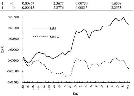
The respective CARs based on MM and MMG models are presented in Figure 1. It can be observed that the CARs of both models have more or less the same pattern. However, since all abnormal returns obtained from the MM are higher than those from the MMG, the CARs for the MMG model are constantly below the MM ones and the difference between the two curves increases. The CARs for the MM model continuously increase while those for the MMG model roughly remain at the same level. A look at the CARs and their respective t-sta-tistics in Table 2 for various periods around the event day also reveals that the two models particularly give a different interpretation for the period (-1, +1). When accounting for GARCH, the CAR for this period is not statistically significant. The differences observed in the CARs of the two models are due to the magnitude of the α and the β estimates. A look at the histograms of these two parameters, which are reported in Figure 2, for the two models reveals that their distributions are slightly different.
A GARCH process is unconditionally homoskedastic. The presence of GARCH does not violate the assumptions of the second order properties of the least square estimator. However, the differences in
abnormal returns we obtain are due to the fact the parameters estimates of α and β obtained using the
market model are inefficient since they are not adjusted for GARCH effects. When the market model residuals are tested for the presence of ARCH using the Lagrange Multiplier approach of Engle (1982), a strong evidence of ARCH properties was revealed. The MMG resolves this problem, and the
firms have, indeed statistically significant GARCH parameters estimates of α and β coefficients and
their sum is also less than the unity.
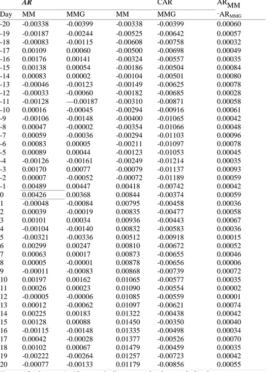
Table 1. Comparison of Abnormal Returns (AR) and Cumulative Abnormal Returns (CAR) using the Market Model (MM) and the GARCH Market Model (MMG)
AR CAR ARMM Day MM MMG MM MMG _ARMMG -20 -0.00338 -0.00399 -0.00338 -0.00399 0.00060 -19 -0.00187 -0.00244 -0.00525 -0.00642 0.00057 -18 -0.00083 -0.00115 -0.00608 -0.00758 0.00032 -17 0.00109 0.00060 -0.00500 -0.00698 0.00049 -16 0.00176 0.00141 -0.00324 -0.00557 0.00035 -15 0.00138 0.00054 -0.00186 -0.00504 0.00084 -14 0.00083 0.00002 -0.00104 -0.00501 0.00080 -13 -0.00046 -0.00123 -0.00149 -0.00625 0.00078 -12 -0.00033 -0.00060 -0.00182 -0.00685 0.00028 -11 -0.00128 —0.00187 -0.00310 -0.00871 0.00058 -10 0.00016 -0.00045 -0.00294 -0.00916 0.00061 -9 -0.00106 -0.00148 -0.00400 -0.01065 0.00042 -8 0.00047 -0.00002 -0.00354 -0.01066 0.00048 -7 0.00059 -0.00036 -0.00294 -0.01103 0.00096 -6 0.00083 0.00005 -0.00211 -0.01097 0.00078 -5 0.00089 0.00044 -0.00123 -0.01053 0.00045 -4 -0.00126 -0.00161 -0.00249 -0.01214 0.00035 -3 0.00170 0.00077 -0.00079 -0.01137 0.00093 -2 0.00007 -0.00052 -0.00072 -0.01189 0.00059 -1 0.00489 0.00447 0.00418 -0.00742 0.00042 0 0.00426 0.00368 0.00844 -0.00374 0.00059 1 -0.00048 -0.00084 0.00795 -0.00458 0.00036 2 0.00039 -0.00019 0.00835 -0.00477 0.00058 3 0.00101 0.00034 0.00936 -0.00443 0.00067 4 -0.00104 -0.00140 0.00832 -0.00583 0.00036 5 -0.00321 -0.00336 0.00512 -0.00918 0.00015 6 0.00299 0.00247 0.00810 -0.00672 0.00052 7 0.00063 0.00017 0.00873 -0.00655 0.00046 8 0.00005 -0.00001 0.00878 -0.00656 0.00006 9 -0.00011 -0.00083 0.00868 -0.00739 0.00072 10 0.00197 0.00162 0.01065 -0.00577 0.00035 11 0.00026 0.00023 0.01090 -0.00554 0.00002 12 -0.00005 -0.00006 0.01085 -0.00559 0.00001 13 0.00012 -0.00062 0.01097 -0.00621 0.00074 14 0.00225 0.00183 0.01322 -0.00438 0.00042 15 0.00128 0.00088 0.01450 -0.00350 0.00040 16 -0.00115 -0.00148 0.01335 -0.00498 0.00034 17 0.00042 -0.00028 0.01377 -0.00526 0.00070 18 0.00102 0.00067 0.01479 -0.00459 0.00035 19 -0.00222 -0.00264 0.01257 -0.00723 0.00042 20 -0.00077 -0.00133 0.01179 -0.00856 0.00055
Note: ARs that are significant at the live percent level are underlined.
Table 2. CARs and t-statistics for Various Intervals
MM MMG
Period CAR t-stat CAR t-stat
-20 +20 0.01179 0.8189 -0.00856 -0.5232
-10 +10 0.01375 1.3334 0.00294 0.2516
-5 +5 0.00723 1.2506 0.00179 0.6229
-1 +1 0.00867 2.3677 0.00730 1.6508
-1 0 0.00915 2.8776 0.00815 2.2553
Figure 1. Comparison of the CARs based on Market Model and Market Model Corrected for GARCH
V. CONCLUSION
The purpose of this paper is to estimate market model parameters adjusted for GARCH effects. Even though there is no intrinsic interest in estimating the conditional variance, the market model should be estimated by maximum likelihood in order to obtain a more efficient estimator of the regression parameters. The lack of efficiency of the least square estimator may result in such a poor estimate that the wrong conclusion may be drawn from an empirical study.
Figure 2b, Histogram of the Betas
Using a sample of divestitures, we empirically investigate how the adjustment for GARCH affects the abnormal returns associated with the event and can lead to a different interpretation of their economic significance.
Acknowledgment
The authors would like to thank two anonymous referees of this journal for their comments and suggestions.
Notes
*Direct all correspondence to: A. Tourani Rad, Limburg Institute of Financial Economics, University of Limburg, P.O. Box 616, 6200 MD Maastricht, The Netherlands.
References
Afshar, K.A., R.J. Taffler and P.S. Sudersanam. 1992. "The effects of Corporate
Divestments on Shareholder Wealth: The UK Experience," Journal of Banking and Finance, 16: 115-135.
Akgiray, Vedat. 1989. "Conditional Heteroskedasticity in Time Series of Stock Returns: Evidence and Forecasts, "Journal of Business, 62: 55-80.
Baillie, Richard T. and Tim Bollerslev. 1989. "The Message in Daily Exchange Rates: A Conditional-Variance Tale," Journal of Business & Economic Statistics, 7: 297-305.
Bera, Anil, Edward Bubnys and Hun Park. 1988. "Conditional Heteroskedasticity in the Market Model and Efficient Estimates of Betas," Financial Review, 23: 201-214.
Berndt, Ernst K., Bronavyn H. Hall, Robert E. Hall and Jerry A. Hausman. 1974. "Estimation and Inference in Nonlinear Structural Models, "Annals of Economics and Social Measurement, 4: 653-665. Bollerslev, Tim. 1986. "Generalized Autoregressive Conditional Heteroskedasticity," Journal of
Econometrics, 31: 307-327.
______. 1987. "A Conditionally Heteroskedastic Time Series Model for Security Prices and Rates of Return Data," Review of Economic and Statistics, 59: 542-547.
Corhay, Albert and Alireza Tourani Rad. 1994. "Statistical Properties of Daily Returns: Evidence from European Stock Markets," Journal of Business Finance and Accounting, 21: 271-282. Denning, Karen C. and Kuldeep Shastri. 1990. "Single Sale Divestment: The Impact on Stockholders and Bondholders," Journal of Business Finance and Accounting, 17: 731-743.
Diebold, Francis X., Jang Im and Jevons Lee. 1988. Conditional Heteroskedasticity in the Market, Finance and Economics Discussion Series, 42, Division of Research and Statistics, Federal Reserve Board, Washington D.C.
Engle, Robert. 1982. "Autoregressive Conditional Heteroskedasticity with Estimates of the Variance of UK inflation," Econometrica, 50: 987-1008.
Engle, Robert and Tim Bollerslev. 1986. "Modelling the Persistence of Conditional Variances,"
Econometric Reviews, 5: 1-50.
Giaccoto, C. and M.M. Ali. 1982. "Optimal Distribution Free Tests and Further Evidence of Heteroskedasticity in the Market Model" Journal of Finance, 37: 1247-1257.
Hearth, Douglas P. and Janis K. Zaima. 1984. "Volontary Corporate Divestitures and Value,"
Financial Management, 13: 10-16.
______. 1986. "Divestiture Uncertainty and Shareholder Wealth: Evidence from the U.S.A. (1975-1982)," Journal of Business Finance and Accounting, 13: 71-85.
Hsieh, David A. 1989. "Modelling Heteroskedasticity in Daily Foreign-Exchange Rates," Journal of
Business & Economic Statistics, 7: 307-317.
Iqbal, Zahid and Prakash L. Dheeriya. 1991. "A Comparison of the Market Model and Random Coefficient Model Using Mergers as an Event," Journal of Economics and Business, 43: 87-93.
Jain, Perm. C. 1985. "Effect of Voluntary Sell-Off Announcements on Shareholder Wealth,"
Journal of Finance, 43: 87-93.
Linn, Scott C. and Michael S. Rozeff. 1986. "The Corporate Sell-Off." Pp. 576-634 in
The Revolution in Corporate Finance, edited by J.M. Stern and D.H. Chew Jr. Oxford, England: Basil
Blackwell.
Rosenfeld, James D. 1984. "Additional Evidence on the Relation Between Divestiture Announcements and Shareholders Wealth," Journal of Finance, 39: 1437-1448. Scholes, Myron and Joseph Williams. 1977. "Estimating Betas from Nonsynchronous
Data," Journal of Financial Economics, 5: 309-328.
Sharpe, William F. 1963. "A Simplified Model for Portfolio Analysis," Management