ACOUSTIC AND SEISMIC SIGNAL PROCESSING FOR
FOOTSTEP DETECTION
by
Ross E. BLAND
B.S., Massachusetts Institute of Technology (2005)
Submitted to the Department of Electrical Engineering and Computer
Science
in partial fulfillment of the requirements for the degree of
Master of Engineering in Electrical Engineering and Computer Science
at the
MASSACHUSETTS INSTITUTE OF TECHNOLOGY
June 2006
@
Ross E. Bland, MMVI. All rights reserved.
The author hereby grants to MIT permission to reproduce and distribute
publicly paper and electronic copies of this thesis document in whole or in
part.
Author -
--Department of Electrical Engineering and Computer Science
May 20, 2006
Certified by.
---..--
Charles E. Rohrs
Research Scientist, Digital
Siga
Processing Group
Thesis Supervisor
Accepted by
.ARCHIVES
Arthur C. Smith
Chairman, Department Committee on Graduate Students
I
MASSACHUSETTS INS[ E OF TECHNOLOGYAUG 14
2006
I
Acoustic and Seismic Signal Processing for Footstep Detection by
Ross E. Bland
Submitted to the Department of Electrical Engineering and Computer Science on May 25, 2006, in partial fulfillment of the
requirements for the degree of
Master of Engineering in Electrical Engineering and Computer Science
Abstract
The problem of detecting footsteps using acoustic and seismic sensors is approached from three different angles in this thesis. First, accelerometer data processing systems are designed to make footsteps more apparent to a human operator listening to accelerometer recordings. These systems work by modulating footstep signal energy into the ear's most sensitive frequency bands. Second, linear predictive modeling is shown to be an effective means to detect footsteps in accelerometer and microphone data. The time evolution of the third order linear prediction coefficients leads to the classical binary hypothesis testing framework. Lastly, a new method for blindly estimating the filters of a SIMO channel is presented. This method is attractive because it allows for a more tractable performance analysis.
Thesis Supervisor: Charles E. Rohrs
Acknowledgments
First and foremost, I should thank my thesis supervisor, Dr. Charles Rohrs. I find it remarkable that Charlie has always had my best interest in mind. He has done his very best to teach me how to conduct quality research. I probably don't realize how fortunate I am to have a supervisor so willing to dive into any problem I bring to him. His enthusiasm for research has been a source of motivation and energy for me. Additionally, our college football conversations certainly helped to reduce the stress associated with graduate school at MIT.
I also should thank everyone in DSPG: Al, Eric, Petros, Sourav, Maya, Joe, Tom, Melanie, Joonsung,
Al K., Dennis, Matt, and of course Zahi. I'd like to thank Al for encouraging me to share my ideas
in group meetings, for teaching me how to think creatively, and for showing me how to communicate precisely. Eric is absolutely instrumental to the group. He always has the answer and if he doesn't he'll find out for you. Petros has stepped in and saved the day on numerous occasions (even from another continent). Sourav has been an awesome colleague. I am always amazed at how willing he is to drop what he is doing to help me with latex or to figure out some problem from research. I should thank Joe for his company in the office on the weekends. Tom was really great to field all of my random questions about acoustics and audio signal processing. Much thanks to Melanie for being the awesome problem solver she is. I thank Joonsung for providing me with a hero. I thank Al K. for the company in the group office at odd hours of the night. Dennis has been a great officemate and I have really enjoyed getting to know him better. I appreciate Zahi keeping the office fun. Lastly, I thank Matt for all of the laughs and good times. I can't imagine going through MIT without him.
I should also thank Dr. James Sabatier from the Department of Physics and Astronomy at The Uni-versity of Mississippi for his help in data collection.
Finally, this research was supported in part by participation in the Georgia Institute of Technology MURI 2004 sponsored by Army Research Office (ARO) under award W91 I NF-04-1-0190 and was supported in part by participation in the Advanced Sensors Collaborative Technology Alliance (CTA) sponsored by the U.S. Army Research Laboratory under Cooperative agreement DAAD19-01-2-008.
Contents
1 Introduction 15
1.1 Problems Considered . ... . . . . . . . . . 16
1.2 PreviousWork ... ... . . . .. ... .16
1.2.1 Kurtosis and Cadence . ... . . . . . . . . . 17
1.2.2 Short-time Fourier Transform Analysis ... . . . . . . . ..... 18
1.2.3 Footstep Feature Extraction for Personal Identification . . . . 20
1.3 Outline of the Thesis . ... . . . . . . . . .... . 22
2 Digital Processing to Aid the Listener in Footstep Detection 23 2.1 The Data ... . . . ... 23
2.2 Motivation for Processing ... . . . . . . . .... . 23
2.3 Digital Processing... . . .. .... ... . 24
2.3.1 Noise Removal .. ... .. ... .. 24
2.3.2 First Method: Shifting 11.025-22.05kHz Band Down in Frequency . . . . . 27
2.3.3 Second Method: Placing High Footstep Energy in the Most Sensitive Fre-quency Range... .. . . ... 27
2.4 Summary .
3 Linear Predictive Modeling to Identify Footsteps
3.1 Linear Prediction Background ... . . . . . . . . . .....
3.2 Linear Predictive Modeling of Footstep Data . . . .... 3.2.1 Microphone Data Noise Removal . . . . . . . . ..... 3.2.2 Sectioning Data Using a Sliding Window . . . . . . . .... 3.2.3 Model Order .... .... . ... 3.3 Visualizing Accelerometer Footsteps in Three-Dimensional Coefficient Space . .
3.3.1 Identifying First and Second Footstep Components in Coefficient Space . 3.3.2 Window Length Effects ... . . . . . . . . . ..... 3.3.3 Consistency of Coefficient Behavior Across Different Footsteps . . . . . 3.3.4 Linear Prediction Applied to Stealthy Footsteps . . . . 3.4 Microphone Footsteps in Three-Dimensional Linear Prediction Coefficient Space
3.4.1 Microphone Recordings of Regular Footsteps . . . . 3.4.2 Microphone Recordings of Stealthy Footsteps . . . .
3.5 Summary ... . . . . ...
4 Blind Channel Identification using Least Squares
4.1 SIMO Channel ... . .... ...
4.2 Least Squares Algorithm ... . . . . .....
4.3 Alternative Estimate: Pinning a Channel Coefficient . . . . 4.4 Comparison of the SVD and Pinning Channel Estimation Methods . . 4.5 Deriving the Distribution of the Channel Estimate . . . .....
4.6 Summary ... ... . . . . .. .. ....
5 Conclusion
5.1 Digital Processing to Aid the Listener in Footstep Detection ... 5.2 Linear Predictive Modeling to Identify Footsteps ... 5.3 Blind Channel Identification Using Least Squares ...
31 . 31 . 34 . 34 . 38 . 39 . 40 . 40 . 42 . 44 . 46 . 50 . 51 . 55 .. 57 59 . . . . 59 . . . . . 61 . . . . . 62 . . . . . 63 . . . . . 66 . . . . 72
A Digital Processing Implementations in MATLAB 77
A.1 Method 1 Processing ... ... 77
A.2 Method 2 Processing ... ... 78
B Available Data Files 81
List of Figures
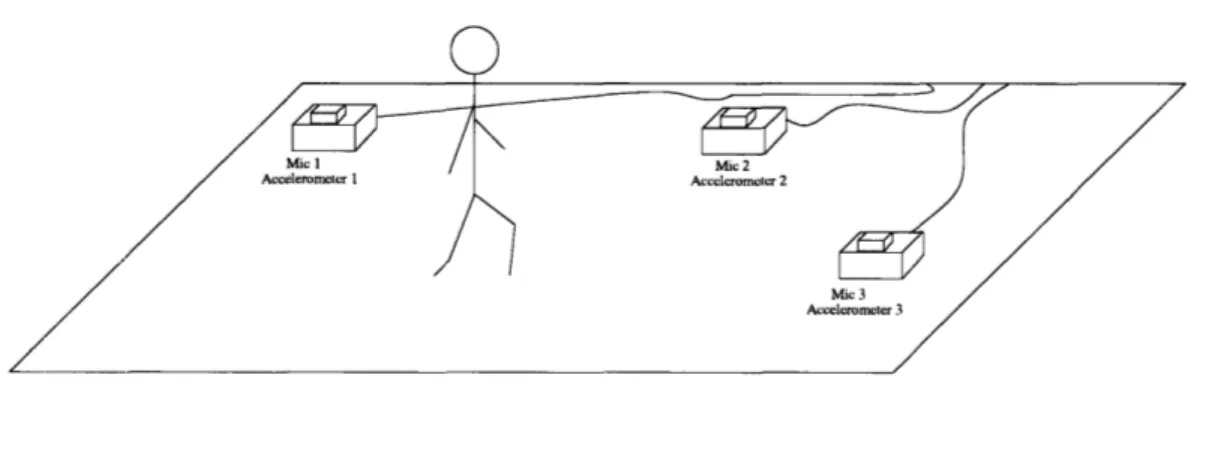
1-1 Three acoustic and three seismic sensors monitoring an area for footsteps . . . . 17
1-2 Houston's Detection Scheme ... . . . . . . . ..... 19
1-3 An example of the normalized STFT of footstep data given by Houston in [3] .... . 19 1-4 Mel-Cepstrum Analysis (from [7]). (a) Amplitude vs. Frequency Plot. (b) Fourth and
fifth peak frequencies generated from multiple sections of the data for each of the five
walkers... . . . . . . . . ... .. ... ... . 20
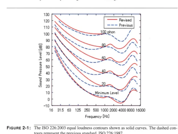
1-5 Distribution of walking intervals for five subjects (from [7]) . . . . 21 1-6 Envelope of the footstep spectrum for five subjects (from [7]) . . . . 21 2-1 The ISO 226:2003 equal loudness contours shown as solid curves. The dashed
con-tours represent the previous standard, ISO 226:1987 .. . . . . . . . . ..... . 24 2-2 Short-time Fourier Transform of a Section of Accelerometer Data Containing a Footstep 25 2-3 Noise Power Spectral Density Estimate Computed using Welch's Method . . . . 26 2-4 First Method Processing: Shifting of the 11.025-22.05kHz band down to 0-11.025kHz. 27 2-5 STFT of a "Stealthy" Footstep ... . . . . . . . . ..... 28 2-6 Second Method Processing: Frequencies with high footstep energy are shifted to the
3-1 Linear Prediction Model ... . . . . . . . . . 32
3-2 (a) All-Pole Signal Model. (b) Inverse of the All-Pole System . . . . 34
3-3 Top: Section of microphone data absent of footsteps. Bottom: Prediction error energy corresponding to data section ... . . . . . . . .... .. 36
3-4 Microphone Noise Reduction System ... . . . . . . . ..... 37
3-5 Microphone data noise reduction. Top: Before filtering. Bottom: After filtering. . . . 37
3-6 Linear predictive model coefficients are computed for windowed sections of the data. 38 3-7 Prediction Error Energy vs. Model Order for Accelerometer Footstep . . . . 39
3-8 Prediction Error Energy vs. Model Order for Microphone Footstep . . . . 40
3-9 Accelerometer Recording of a Single Footstep ... . . . . . . . .... 41
3-10 Identification of first and second footstep components in coefficient space . . . . 42
3-11 Multiple window lengths on the same footstep ... . . . . . . . ..... 43
3-12 For various window lengths, V is computed from a section of data absent of footsteps. 45 3-13 A comparison of coefficient paths for three different footsteps. Window size of L = 5000 . . . . . . . . .. . . . .. ... . ... . . . .. 46
3-14 Accelerometer Footstep Data. Top: Regular Walking Style. Bottom: Stealthy Walk-ing Style . . . .. . .. ... . ... . .. . . . . ... .. . . . .. 47
3-15 Comparison of regular and stealthy footstep linear prediction coefficient paths. Re-gions of the regular footstep are labeled with arrows . . . .... . 48
3-16 Stealthy footstep recorded with accelerometer. First component is shown in red, sec-ond component in blue ... . . . . . . . ..... 49
3-17 Coefficient path for stealthy accelerometer footstep .. . . . . . . . .... . 50
3-18 Three different regular microphone footsteps. The corresponding coefficient paths are shown in Figure (3-19) . ... . . . . . . . . . 51
3-19 Linear prediction coefficient paths for three regular footsteps recorded with a micro-phone. Plots (a) and (b) are different views of the same data . . . . 53
3-20 Section of microphone data used to investigate coefficient behavior between footsteps. 54 3-21 Coefficient path produced from the data section in Figure (3-20) . . . . 55
3-22 Coefficient paths generated from data sections in Figure (3-19) . . . . 56
3-23 Comparison of regular and stealthy footstep coefficient paths for microphone data. . 57 4-1 SIMO Channel ... ... . . . . . . ... .60
4-3 Performance Comparison of SVD and Pinning Methods . . . . 64 4-4 Performance Comparison of SVD and Pinning Methods with hi [K] = 0.1 . . . . 65 4-5 The R distribution. (a) PDF estimates of R(5), R(10), and R(20). (b) Variance of
the distribution of R(n) for n from 3 to 30 .... . . . . . . . ..... 69 4-6 Histogram plots comparing the estimated probability density for hi [0] and an R
ran-dom variable scaled by m- . (a) N + 1 = 3 (b) N + 1 = 10 (c) N + 1 = 30 (d) o2
N + 1= 1 00... .... ... . ... . ... 70 4-7 Plots comparing the histograms of YL to the PDF of a zero mean, unit variance
Gaussian random variable. Each plot corresponds to a different value for N. (a)
CHAPTER 1
Introduction
Many applications can be envisioned for a system that is able to detect human activity in some area. Probably the most obvious application is the detection of intruders in a secure region. It is often the case that a system capable of detecting pedestrians is desired. Any system to accomplish this task obviously needs a way to sense the pedestrian. Acoustic and seismic sensors are capable of measuring pedestrian activity and are often employed for this task for a number of reasons. Such sensor systems are inexpensive, passive (do not emit energy), and potentially easily installed. In the case that the system should alarm only when a pedestrian is present, processing of the acoustic and seismic signals should make it possible for the system to discrim-inate footsteps from other acoustic and seismic sources such as highways, railroads, operating machinery, and trees and bushes swaying in the wind. As for indoor detec-tion, heating and air conditioning units are a common noise source. The decision to alarm can be made by a human operator or by a signal processing algorithm. How-ever, even when the system involves a human operator, signal processing should be performed to make the task easier and more error-free for the operator.
Discriminating footstep signals from noise sources is a challenging problem to solve with human operators or software. The footstep signal to noise ratio decreases rapidly with the distance between the sensors and the pedestrian. In addition, impulsive noise often looks and sounds like footsteps. Another complication is that footstep signals can vary greatly from one person to the next as well as one environment to the next. While this is a challenging problem, with high-performance sensors and sophisticated signal processing, it is hardly impossible.
A system that is successful in discriminating footsteps from noise sources may also be extended to solve similarly related problems. For example, it may be possible to identify a pedestrian based on the recorded footstep signals. In addition, evaluation of the acoustic and seismic signals produced by a person walking may aid in the diagnosis of gait-affecting diseases.
1.1 Problems Considered
There are three closely related problems explored in this thesis. One form of a human operator is a person listening to acoustic and seismic data in order to monitor an area for footsteps. The first problem is how can acoustic and seismic signals be processed to aid the listener in footstep detection. While it may seem odd that the operator is listening to seismic data, the seismic data is actually sampled at 44.1kHz (stan-dard audio CD sampling rate) and contains significant energy in the audio frequency range.
There are no constraints on the processing that is performed on the acoustic and seismic data. The goal is simply to process the data in anyway that will enhance the listener's ability to detect footsteps and discriminate them from other acoustic and seismic sources. One issue with this problem is the difficulty in measuring the performance of processing methods. Performance can only be measured qualitatively by listening to the original data file and processed data file and comparing the two. The second problem considered in this thesis is the characterization of footsteps recorded with acoustic and seismic sensors. In order to discriminate footsteps from similar acoustic and seismic noise sources, footstep signal feature extraction must be developed. The extracted features can be employed in a decision rule that states when the presence of a footstep is declared. A possibly more difficult but similarly related problem considers using the extracted features to infer qualities of the walker such as height, weight, or even identity.
Lastly, this thesis looks at the problem of finding alternative methods for blind chan-nel identification. A method that is computationally inexpensive and allows for a tractable analysis of performance is desired. Blind channel identification is impor-tant for footstep detection in that blind channel identification is useful for sensor fusion. Sensor fusion is the process of combining signals from multiple sensors. Fig-ure (1-1) depicts a situation in which three accelerometers (seismic sensors) and three microphones (acoustic sensors) are monitoring an area for footsteps. Blind channel identification can be used in the process of combining all six signals to produce a seventh signal that is then processed to determine if an intruder is present.
1.2 Previous Work
The problem of detecting footsteps using acoustic or seismic sensors has been studied before. In this section, the most relevant published material is discussed.
FIGURE 1-1 : Three acoustic and three seismic sensors monitoring an area for footsteps.
1.2.1 Kurtosis and Cadence
In [8], Succi considers using the kurtosis and the cadence of seismic signals to detect footsteps. Kurtosis is the degree of peakedness of a distribution and is defined as a normalized form of the fourth central moment. While there are several flavors of kurtosis, Succi uses the kurtosis proper denoted f2 and defined by
32-
= _4(2
(1.1)
where
pi
denotes the ith central moment [9].For N samples, Succi estimates the kurtosis of the amplitude distribution of a seismic signal s[n] as
k1
N=l(S[n] - M)402
(I
IEN=i(s[n]
-
t)2
2 (1.2)where
p
is the sample average of the signal over the range 1 < n < N. This estimate measures the shape of the signal. Scaling the data has no effect on the estimate. Since kurtosis is a measure of the peakedness of a distribution, the kurtosis of a section of data is increased by impulsive events. Succi reasons that kurtosis is a good indicator of footsteps since footsteps appear as sharp spikes in the data unlike several seismic noise sources such as wind blowing over the ground or vehicle noise. Succi computes /2 for overlapping four second sections of the data. He finds that for each of three recordings, background noise, light passenger vehicle, and heavy armored personnel carrier, the mean of /2 is approximately 3. Succi reports a mean 1.2 Previous Work12 of 6 for recordings of footsteps. The variance of 12 is 0.4 for ambient noise, 0.6
for the light passenger vehicle, 1.9 for the armored personnel carrier, and 2.5 for the footsteps.
Succi's kurtosis method of detecting footsteps essentially reduces the data to a single parameter that is then used to decide if a walker is present. This method is attractive because of its simplicity. However, this detection scheme is fairly limited since it uses only one parameter to characterize four second sections of the signal. A major problem is that any noise source that generates spikes in the data will be interpreted as a footstep.
Succi also offers an alternative single parameter footstep detection scheme. Succi reasons that the cadence of the signal can be used to detect footsteps. Each footstep produces a spike in the seismic signal. The time between spikes is measured and used to determine if a walker is present. This detection scheme also has its limita-tions. One of the most apparent problems is that the success of the cadence detection scheme is limited by noise sources that generate large amplitude values in the data.
1.2.2 Short-time Fourier Transform Analysis
Houston in [3] takes a somewhat different approach to footstep detection in which he utilizes the short-time Fourier transform (STFT). Houston's detection scheme fo-cuses on the periodic arrival of footsteps instead of on the information in individual footstep signals.
A block diagram summarizing Houston's processing is shown in Figure (1-2).
Hous-ton finds that the 10-40Hz band contains most of the footstep energy and therefore passes the data through a bandpass filter with these cutoff frequencies. The absolute value of the signal is then taken before downsampling the signal to a sampling rate of 40Hz. The STFT of the data is then computed (26 second window, 95% overlap) and normalized using a split-window 2-pass normalizer (a conventional STFT anal-ysis algorithm). Figure (1-3) shows the example of a resulting normalized STFT plot given by Houston.
A set of ad hoc decision rules are applied to the normalized Fourier transform of each 26 second window of data (one horizontal line in Figure (1-3). The presence of a walker is declared when the following criteria are met:
1. A primary frequency component must occur in the 0.5 to 3.0 Hz range.
2. The primary frequency component must have a second or third harmonic present. 3. The primary frequency component must be greater than 11 dB over the noise
level and the harmonic greater than 7dB, or vice versa.
Houston shows the results of applying his detection scheme to real footstep data recorded with seismic sensors in an outdoor environment. He concludes that his method shows promise but more data sets are needed to fully characterize its perfor-mance. Houston also mentions a couple of the potential pitfalls associated with his
Seismic Signal Sampled at 1200Hz
FIGURE 1-2:
STFT STFT Apply
26 sec window Normalization Decision
95% overlap Rule
Houston's Detection Scheme
Spectroam of Envelope Data -Stadard Walk - 6 December Run 3
AP=40 6 D0c K Non W3 Wa% -SpcAMn OwmeAI er t-00-215.6 Sec
rtuyMWA tC
5 6 7 8 9 10 c11
sun,, a 12 13 4
15
FIGURE 1-3: An example of the normalized STFT of footstep data given by Houston in [3].
detection scheme. He explains that it is possible for noise sources such as traffic on nearby roadways to mask the footstep signals. In addition, Houston mentions that stealthy walking, in which the walker takes soft footsteps, will not be detected with 1.2 Previous Work
his method.
1.2.3 Footstep Feature Extraction for Personal Identification
A problem closely related to footstep detection is that of using footstep signatures for
identification purposes. In [7], Shoji considers using peak frequencies generated by a mel-cepstrum analysis, the time between successive footsteps, and samples of the spectrum envelope to identify walkers.
Mel-Cepstrum Analysis
Shoji applies a type of mel-cepstrum analysis to the footstep data to generate an amplitude versus frequency plot. The example plot given in [7] is shown in Figure (1-4(a)). Each curve in the plot corresponds to a different walker. The peak frequencies of the curves are used as feature parameters. For example, a plot given in [7] showing the fourth and fifth peak frequencies generated from multiple sections of the data for each of the five walkers is presented in Figure (1-4(b)). In this plot, subject C is the only subject that can be clearly discriminated from the others.
I
(a) (b)
FIGURE 1-4: Mel-Cepstrum Analysis (from [7]). (a) Amplitude vs. Frequency Plot. (b) Fourth
and fifth peak frequencies generated from multiple sections of the data for each of the five walkers.
Walking Intervals
The second feature parameter Shoji considers is the time between footsteps. The time between footsteps is measured by estimating the pitch using an autocorrelation method. A figure given by Shoji in [7] is shown in Figure (1-5). This figure shows 1 Introduction 1000 1800. 1200- 1000-0 am.
the distribution of the measured walking intervals for five subjects. subject B is easily discriminated from the others.
0.55
To* is"c)
In this plot, only
FIGURE 1-5: Distribution of walking intervals for five subjects (from [7]).
Envelope of the Footstep Spectrum
Lastly, Shoji considers using information in the envelope of the footstep spectrum to identify walkers. In [7] Shoji gives Figure (1-6) to illustrate the differences in the envelope of the footstep spectrum across different subjects. A vector of samples of the footstep spectrum envelope is computed and used to characterize footstep signals.
rque"nc IMA
00
FIGURE 1-6: Envelope of the footstep spectrum for five subjects (from [7]).
1.2 Previous Work
' *IA
mx x xx M x + @~~
0 iC 0 00oe 00 0 *444 ,, +,The frequencies from the mel-cepstrum analysis, the walking interval times, and the samples of the footstep spectrum envelope are combined in a vector. Vector quantization is then used to cluster the parameters. This allows all three sources of information - the mel-cepstrum frequencies, the walking interval times, and the footstep spectrum envelope -to be simultaneously used to make a decision on the walker's identity.
1.3 Outline of the Thesis
This thesis explores the general problem of using acoustic and seismic sensors to detect footsteps. However, each chapter in the thesis considers a different aspect of the problem. Chapter 2 looks at digital processing that can help a human opera-tor detect footsteps when listening to sensor data. More specifically, the short-time Fourier transform (STFT) is used to analyze accelerometer data (an accelerometer is a type of seismic sensor). The idea is that since the accelerometer data is sampled at 44.1kHz (CD quality sampling rate), the footsteps can be heard when playing the data through a speaker. With the use of STFT analysis, accelerometer data processing can be developed to make the footsteps more easily detected by the listener. In Chapter 3, linear predictive analysis is considered for the automatic detection of footsteps in accelerometer and microphone data. Windowed sections of the sensor data are used to compute linear prediction coefficients. The feasibility of using the coefficients of a linear prediction model to discriminate footsteps from noise artifacts
in the data is established.
Lastly, Chapter 4 explains the least squares solution to blind channel identification. Chapter 4 also investigates an alternative method to perform blind channel identifi-cation. This alternative method is attractive because it allows for a recursive solu-tion. Additionally, this alternative method was motivated by the potential for a more tractable performance analysis.
CHAPTER 2
Digital Processing to Aid the
Listener in Footstep Detection
A person walking through a room generates both acoustic and seismic vibrations mostly due to footsteps. These vibrations can be recorded with microphones and accelerometers, respectively. These recorded signals can be monitored to detect the presence of an intruder. This chapter presents digital processing that can be per-formed on the recorded signals in order to make the footsteps more apparent to a human listener.
2.1 The Data
The data discussed in this chapter was collected by placing a microphone and ac-celerometer in the center of a room. A person then walked in a circle (approximate diameter of 6 feet) around the sensors. Two data sets were recorded: one in which the person walked "regularly" and another in which the person walking tried to make a minimal amount of noise. The two data sets are identified as "regular" and "stealthy." The recorded data was digitized at 16 bits with a 44.1 kHz sampling rate.
2.2 Motivation for Processing
Figure (2-1) shows two standards for equal loudness contours for listening in free sound fields. The solid contours are the most recent standards. As can be seen from these contours, the human ear is more sensitive to sounds near 3kHz than sounds at
lower or higher frequencies. The contours in Figure (2-1) were produced by testing subjects 18-25 years of age with normal hearing.
31.5 63 125 250 500 1000 2000
Frequency [Hz]
4000 8000 16000
FIGURE 2-1: The ISO 226:2003 equal loudness contours shown as solid curves. tours represent the previous standard, ISO 226:1987.
The dashed
con-Considering this filtering performed by the ear, it makes sense that moving the recorded data from low-sensitivity frequency ranges to high-sensitivity frequency ranges could
aid the listener in detecting footsteps. The processing discussed in this chapter is based on this idea.
2.3 Digital Processing 2.3.1 Noise Removal
Before shifting low-sensitivity frequency ranges to high-sensitivity ranges, an at-tempt at noise removal should be made. The most common sources of noise in an indoor environment are the heating and cooling systems and the electrical noise in the sensor. Both of these noise sources are stationary over sufficiently short time
intervals. The first step in removing the noise is to examine the frequency content of the data. At frequencies where the noise power is significantly greater than the signal (footstep) power, the data should be attenuated. The frequency content of the noise 2 Digital Processing to Aid the Listener in Footstep Detection
130
120
110100
90
80 70 60 50 4030
20 10 0 -10 16 ~·_I·_···can be estimated by performing spectral analysis on data recorded in the absence of footsteps. The frequency content of the footsteps can be estimated by using the short-time Fourier transform (STFT) on sections of data that are known to contain footsteps.
The STFT of a section of accelerometer data containing a footstep can be seen in Figure (2-2). The STFT was taken by windowing the data with a Hamming window of length 200 samples. The windowed segments overlapped 150 samples and the 1,024 point Fast Fourier Transform was used. From the figure, it is apparent that a footstep consists of two components. The first contains a wide range of frequency content in a short amount of time. The second component contains frequency content mostly in the range of 6-16kHz and spread over about 60 milliseconds. Considering the time-frequency nature of these two components as well as a time separation of about 100 milliseconds, it seems likely that the first component is the heel touching down and the second component is the foot coming to a halt against the floor.
0.05 0.1 0.15
Time (s) 0.2 0.25
FIGURE 2-2: Short-time Fourier Transform of a Section of step
Accelerometer Data Containing a
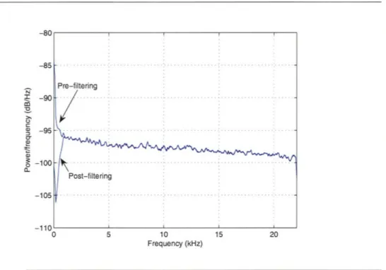
Foot-Since the noise is mostly stationary, spectral analysis can be used to determine its fre-quency content. The curve labeled "pre-filtered" in Figure (2-3) is the power spectral density estimate of the noise computed from a section of the data absent of footsteps. 2.3 Digital Processing
This estimate is computed using Welch's method. More specifically, a Hamming window of length 500 samples is used to compute modified periodograms. An over-lap of 250 is used and the resulting periodograms are averaged to obtain the power spectral density estimate.
As can be seen from this estimate, the noise is fairly evenly distributed over the entire frequency range (0-22.05kHz) except for a spike at low frequencies. In filtering out the noise, there is a fundamental tradeoff between removing the noise and altering the signal of interest. Considering the frequency content of the footstep and as well as that of the noise, it makes sense to attenuate the data in the range from 0 to 500 Hz, since this is where the spike in the noise is located. The noise spectrum after applying a 1 0 0th order FIR high-pass filter with cut-off frequency at about 500Hz to
the data is labeled "post-filtered" in Figure (2-3).
N I m ~0 0 C 0 0~ 0 0 0 a-Frequency (kHz)
FIGURE 2-3: Noise Power Spectral Density Estimate Computed using Welch's Method
It is also important to consider the effect that this high-pass filter has on the footstep component of the data. The second component of the footstep, which is located above 6kHz, is not affected by the filtering. The first component, which contains energy below 500Hz, is affected by the noise removal filtering. However, as can be seen in Figure (2-3), 0-500Hz is a small fraction of the frequency range spanned by the first component. Thus, attenuating the 0-500Hz portion does not have a drastic effect on the first component of the footstep.
2.3.2 First Method: Shifting 11.025-22.05kHz Band Down in Frequency
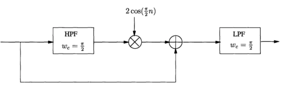
The first approach to make the footsteps more distinct to the listener is to simply take the 11.025-22.05kHz section of the data and shift it down into the 0-11.025kHz range. This operation is shown in Figure(2-4). HPF and LPF denote high-pass filter and low-pass filter, respectively. The cosine used in the frequency shifting has an amplitude of 2 since multiplication by a cosine shifts a signal's spectrum as well as scales it by ½. The 0-11.025kHz band of the output signal contains the superposition of the input signal's 0-11.025kHz and 11.025-22.05kHz bands. The output signal is band-limited to 11.025kHz.
2 cos(3u)
FIGURE 2-4: First Method Processing: Shifting of the 11.025-22.05kHz band down to
0-11.025kHz.
The original accelerometer data file, as well as the processed data file are available for comparison [1]. The actual implementation of the processing in Figure (2-4) can be found in Appendix A. The processing in Figure (2-4) was also applied to the accelerometer data recorded with a "stealthy" walker. The original recording of the stealthy walker as well as the processed recording are also available [1]. A description of the files available from [1] is given in Appendix B.
Listening to the data files before and after processing reveals that the processing of the "regular" walking had a noticeable affect on the recording. It is quite possible that for most listeners this processing can make the detection of footsteps easier. A noticeable affect is also heard in the "stealthy" case. However, in this case it seems that the processing does not make the footsteps significantly easier to detect.
2.3.3 Second Method: Placing High Footstep Energy in the Most Sensitive Frequency Range
The second approach involves taking frequency bands with high footstep energy and shifting them to the frequencies that are most sensitive to the ear. As can be seen in Figure (2-1), 1-6kHz is a region of high-sensitivity for the human ear. Figure (2-2) shows the two components of the footstep signal. The first component is spread fairly evenly over the entire frequency range while the second component is mostly in the 2.3 Digital Processing
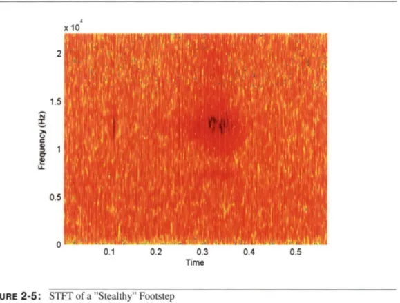
range of 6-16kHz. Figure (2-5) shows the STFT of a "stealthy" footstep. As can be seen in this figure, the first component of the footstep is nearly eliminated but the second component still has a strong presence. Therefore, it seems the 6-16kHz band contains significant footstep energy regardless of the type of walking. Thus, it seems plausible that shifting this band into the high-sensitivity 1-6kHz region could aid the listener in detecting footsteps.
x 10
0.1 0.2 0.3 0.4 0.5
Time
FIGURE 2-5: STFT of a "Stealthy" Footstep
A linear scaling of the frequency axis cannot be used to pack the 6-16kHz band into the 1-6kHz band since this would result in expansion of the data in the time domain. In order to pack the 10kHz band into the 5kHz space, the 10kHz band is decomposed into two 5kHz pieces. These two components are then both placed in the 1-6kHz region.
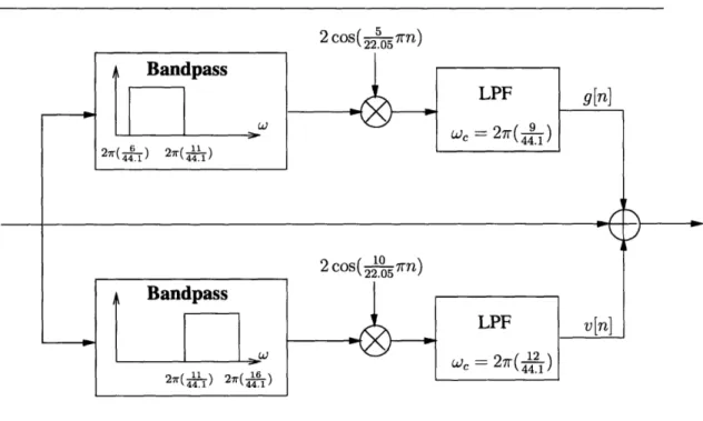
The system that performs this processing is shown in Figure (2-6). The top signal path generates g[n], which contains the input signal's 6-11 lkHz content located at 1-6kHz. The bottom signal path generates v[n], which contains the input signal's 11-16kHz content located at 1-6kHz. The output is the sum of the input signal, g[n] and v[n].
An implementation of the processing shown in Figure (2-6) can be found in Appendix A. Accelerometer data files demonstrating the affect of this processing are available 2 Digital Processing to Aid the Listener in Footstep Detection
[1]. Listening to these files reveals that the footsteps are noticeably more distinct in the processed files for both regular and stealthy walking.
2 cos(22 5 rn)
FIGURE 2-6: Second Method Processing: Frequencies with high footstep energy are shifted to the
frequencies most sensitive to the ear.
2.4 Summary
This chapter explains how equal loudness curves for the human ear can be used to design data processing systems to enhance an operator's ability to detect footsteps when listening to accelerometer data. Two different methods are proposed for mak-ing footsteps in accelerometer data more distinct to the listener. The first method of processing simply shifts the 11-22kHz frequency band of the data down in frequency. This makes footstep energy originally located in the higher frequencies more easily heard. The second method of processing takes the high energy components of the footstep signal and shifts them into the ear's most sensitive frequency band. Be-fore applying either method to accelerometer data, the noise is first reduced using a high-pass filter. The design of this high-pass filter is also discussed in this chapter.
2 Digital Processing to Aid the Listener in Footstep Detection
CHAPTER 3
Linear Predictive Modeling to
Identify Footsteps
Linear prediction can be used to identify footsteps in accelerometer and microphone recordings. Sections of the data are used to compute the coefficients of a linear pre-diction filter. Footstep signals in the data show up as changes in the filter coefficients. The values the coefficients take on over time can be used to discriminate a person walking from some other type of acoustic or seismic source. This chapter begins with a description of the linear predictive model as well as how the filter coefficients are computed.
3.1 Linear Prediction Background
Forward prediction, a well studied problem in time series analysis, considers the problem of predicting the future value of a stationary discrete-time stochastic process, given a collection of past sample values of the process. For example, a pth order predictor uses the sample values s [n - 1], s [n - 2], ..., s [n - p] to estimate s [n]. In general, the predictor can be written as some function f(.) of the given sample values
s[n - 1], s[n - 2], ... ,s[n - p] as follows:
&[n]
= f (s[n - 1], s[n - 2],..., s[n - p]). (3.1)A common simplification is to restrict f(.) to be a linear function of the past sample values, i.e.
p
k=1
(3.2)
The problem is then referred to as forward linear prediction [2].
There exists a deterministic version of the forward linear prediction problem and this is the linear prediction modeling that is used in this chapter. This problem can be framed as follows:
Deterministic Linear Prediction Problem Statement
Given a finite-duration signal s [n], choose the filter coefficients al, a2, ..., ap in Fig-ure (3-1) such that the total energy in the output signal,
E
(e[n])2, is minimized.e [n]
FIGURE 3-1: Linear Prediction Model
In Figure (3-1), 9[n], the output of the predictor filter, is the linear estimate of s[n] based on the past p values of s[n]. The filter coefficients are chosen to minimize the total energy in the prediction error signal. Assuming s[n] is a finite-duration signal defined for 0 < n < N, the prediction error signal energy can be written as
SE
s[n] -
aks[n - k].
n=0 k=1
(3.3)
The error signal energy can be minimized by differentiating with respect to each coefficient and setting the resulting equations to zero.
ae
Nai
E-2
n=0O=0
(sn]
p
- Eaks[n - k] s[n - i]
k=1 i = 1,2,...,p. (3.4)3 Linear Predictive Modeling to Identify Footsteps
This set of equations can be rearranged to obtain
N p N
E E aks[n - k]s[n - i] = E s[n]s[n - i] i = 1, 2,..., p. (3.5)
n=0 k=1 n=0
Defining the deterministic autocorrelation as OO
s [m] = 1 s[n + m]s[n] (3.6)
n=-oo
allows the set of p equations to be rewritten as p
ak ss[i - k] = ss [i] i = 1,2, ...,p. (3.7)
k=1
These equations yield the predictor filter coefficients and are known as the Yule-Walker or Autocorrelation Normal Equations.
The predictor filter coefficients are often used to represent the signal s [n] by a finite number of parameters. This may be better understood by considering the relation-ship between linear prediction and all-pole modeling, a form of parametric signal modeling.
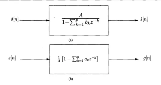
In all-pole modeling, a signal is modeled as the impulse response of a linear time-invariant (LTI) system with p finite poles. This is depicted in Figure (3-2(a)). The parameters bk determine the locations of the system's poles.
In order to simplify the math, the bk's are often determined by considering the in-verse problem shown in Figure (3-2(b)). With this approach, the bk's can found by minimizing the total energy in the signal g[n] - 6[n]. If s[n] is causal, i.e. s[n] = 0 for n < 0, it turns out minimizing g [n] - 6[n] results in Equations (3.7) and bk = ak
for k = 1, 2, ...p. Thus, the linear predictor coefficients can also be interpreted as parameters used to model s [n] as the impulse response of a pth order all-pole system. When modeling a signal using linear prediction or all-pole modeling, the model order p must be chosen. Regardless whether the problem is framed as linear prediction or all-pole modeling, the most direct approach to choosing the order is to use the linear prediction coefficients or all-pole model parameters as the ak's in Figure (3-1) and examine the prediction error energy for various model orders. This can be done by plotting the prediction error energy for the pth order model
00
P
2
Sp = s [sn] - E
f)si[n
- k]. (3.8)n=-vm k=1
versus the model order p. Note that the prediction error energy for the 0t h
order
6[n] A .- [n] (a)
s
[n]
[1i
-z
=I akz-k] g[n] (b)FIGURE 3-2: (a) All-Pole Signal Model. (b) Inverse of the All-Pole System.
model, go, is just the total energy in the signal being modeled,
E
(s [n])2. If the linear predictive or all-pole is a perfect model for s [n] then the energy in the prediction error will go to zero for some p. It is often the case that there is some value of p above which increasing p has little or no effect on the prediction error energy. This value of p is considered an efficient choice for the model order [6].3.2 Linear Predictive Modeling of Footstep Data
In this chapter, the same accelerometer and microphone data discussed in Chapter 2 is used to explore the idea of using linear predictive modeling to detect footsteps. Both the "regular" data set and the "stealthy" data set are discussed in this chapter. As mentioned in Chapter 2, the regular data set was produced by walking in a circle around the microphone and accelerometer while the stealthy data set corresponds to the walker trying to walk softly producing as small a footstep signal as possible. This section discusses a method for removing noise in the data as well as how the data is broken into sections by windowing. In addition, this section looks at model order, an important variable that must be chosen before calculating the linear prediction coefficients for a signal.
3.2.1 Microphone Data Noise Removal
Noise removal for the accelerometer data can be performed with high-pass filtering and is discussed in Chapter 2. The high-pass filter is chosen by comparing the noise power spectral density and the power spectral density of a section of data containing a footstep. The high-pass filter cut-off frequency is chosen such that the data are at-tenuated at frequencies where the noise power spectral density is significantly greater
3 Linear Predictive Modeling to Identify Footsteps
than the footstep power spectral density.
Noise reduction should also be performed on the microphone data before applying linear predictive modeling for footstep detection. Accelerometer data noise removal uses a high-pass filter since most of the accelerometer noise energy is at low frequen-cies. The same is true for the microphone data noise and therefore, a high-pass filter is also used for microphone noise removal. However, a different approach is taken to design the noise removal filter for the microphone data.
The noise sections of the accelerometer data before high-pass filtering, i.e the sec-tions of the filtered data absent of footsteps, are not well modeled by linear pre-diction. That is, for all model orders p the linear prediction error signal, the output signal in Figure (3-1), always has energy that is a significant portion of the modeled signal's total energy,
E(s[n])
2. This is not the case for microphone data. A section of noisy microphone data is shown in the top pane of Figure (3-3) Using this section of noise, the prediction error energy for various model orders p is plotted in dB in Figure (3-3).Q) E 0 0.5 1 1.5 Time [seconds] 0: - -20 --40 --60 0 5 10 15 20 25 Model Order p
FIGURE 3-3: Top: Section of microphone data absent of footsteps. Bottom: Prediction error en-ergy corresponding to data section.
As can be seen in Figure (3-3), the first order model produces error energy 40dB below the total noise section energy (the zeroth order error energy). The reason for such great performance with just a first order model can be understood by looking at the time domain plot of the noisy section of data as well as the first order model coefficient. For the first order model, al = 1. This means the overall system from
microphone noise to linear prediction error can be described by the system function H(z) = 1 - z- 1 or difference equation y[n] - x[n] - x[n - 1]. This system is shown in Figure (3-4) and is a simple differentiator or high-pass filter. This filter makes sense after realizing that the energy in the microphone noise shown in Figure (3-3) is mainly due to low frequency components at approximately 5Hz. A simple high-pass filter such as that shown in Figure (3-4) will strongly attenuate these low frequency components. The ability of the system in Figure (3-4) to decrease noise energy suggests that microphone noise could be reduced by passing the microphone data through this system.
The system shown in Figure (3-4) decreases the noise energy but at the same time alters the footstep signals. This system is an effective method of noise reduction only if it removes enough noise to outweigh its effects on the footstep signals. The two signals in Figure (3-5) demonstrate the effect the noise removal filtering has on microphone data. The top signal is the pre-filtered microphone data and the bottom 3 Linear Predictive Modeling to Identify Footsteps
Microphone
Data
Noise Reduced Microphone Data
FIGURE 3-4: Microphone Noise Reduction System
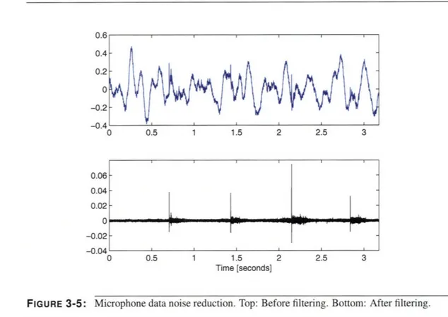
signal is the same data post-filtering. At least from a visual perspective, the suggested noise removal filtering is a success in that the footsteps are much more apparent after filtering.
0 0.5 1 1.5 2 2.5 3
Time [seconds]
FIGURE 3-5: Microphone data noise reduction. Top: Before filtering. Bottom: After filtering.
3.2.2 Sectioning Data Using a Sliding Window
A sliding window is used to apply linear predictive modeling to the data. The linear prediction coefficients are computed for each windowed section of data. The idea is that footsteps can be detected by monitoring the coefficients as they are computed for each section of data. A footstep is declared if the coefficients take on values characteristic of a footstep, or if the trajectory of the coefficients is characteristic of a footstep. There are two parameters that affect the windowing of the data. These parameters are shown in Figure (3-6). Values need to be chosen for the window length, L, as well as the amount of overlap between subsequent windows, M. In addition, the order p of the linear predictive model computed for each section of data needs to be chosen.
Time [seconds]
FIGURE 3-6: Linear predictive model coefficients are computed for windowed sections of the data.
3.2.3 Model Order
A good first step to exploring linear prediction for footstep detection is to examine for various model orders how well a linear predictive model can model a footstep signal. This is done by looking at the prediction error energy. Figure (3-7) shows the prediction error energy plotted versus the model order for a 7, 000 sample section of the accelerometer data. The 7,000 sample section of data is just long enough to include one footstep. As seen in Figure (3-7), the most significant drops in error energy occur when p increases from 1 to 3. In addition, the plot shows that when modeling this entire footstep with linear prediction, near best possible performance is attained with a model order of 16. This means that only small gains are made by increasing the model order beyond 16 when characterizing this footstep with linear prediction coefficients.
Model Order
FIGURE 3-7: Prediction Error Energy vs. Model Order for Accelerometer Footstep
Figure (3-8) shows the prediction error energy plotted versus model order for a sec-tion of microphone data just long enough to include one footstep. According to this plot, p = 3 could be considered an efficient choice for model order when modeling a footstep in microphone data.
In Figure (3-7) one could also argue that p = 3 is an efficient choice for model order since the largest drops in error energy occur when going from p = 1 to p = 3. Using a third order linear predictive model has the added advantage that the coefficients can be viewed as a vector in three-dimensional space. It is for this reason that in this 3.2 Linear Predictive Modeling of Footstep Data
0.01 0.01 0) -, 0.01 C 0.00 0.00 A An 0 5 10 15 20 25 Model Order
FIGURE 3-8: Prediction Error Energy vs. Model Order for Microphone Footstep
chapter a third order model is primarily used for analysis of the accelerometer and microphone data.
3.3 Visualizing Accelerometer Footsteps in Three-Dimensional Coefficient Space
The third order linear predictive model has the advantage that the movement of its coefficients over time can be easily visualized in three-dimensional space. In this sec-tion, a third order linear predictive model is used to analyze accelerometer footstep signals. Several issues, such as window length effects and consistency of coefficient behavior across different footsteps, are considered. First, the regular footsteps are analyzed and then the differences between the linear prediction results seen in the regular and stealthy footsteps are discussed. All accelerometer data considered in this section have been filtered for noise reduction using the high-pass filter discussed in Chapter 2.
3.3.1 Identifying First and Second Footstep Components in Coefficient Space
An accelerometer recording of a footstep is shown in Figure (3-9). In Chapter 2, two components of a footstep signal could be seen in the short-time Fourier transform plots. These two components can also be seen in Figure (3-9). The part of the footstep signal referred to as the "first component" in Chapter 2, is shown in black. 3 Linear Predictive Modeling to Identify Footsteps
The "second component" is shown in blue. The noise regions are shown in red. The edges of the regions in Figure (3-9) were chosen simply by examining the recording visually and noting approximately where the behavior of the signal transitioned.
0.06 0.04 0.02 2000 4000 6000 8000 10000 Sample Number 12000 14000 16000
FIGURE 3-9: Accelerometer Recording of a Single Footstep
As can be seen in Figure (3-9), the footstep is about 7,000 samples long (160ms). Figure (3-10) shows how the prediction coefficients change as a 1,000 sample long window slides over the data with an overlap of 900 samples. When the window over-laps the region in Figure (3-9) colored in black, the resulting coefficients are plotted as black circles. Likewise, when the window overlaps the blue region in Figure (3-9), the coefficients are plotted as blue asterisks. The same goes for coefficients plotted as red diamonds.
Since the window is 1,000 samples long and there are approximately 2,200 samples between the first and second components, the resolution in the time domain is fine enough that the two components of the footstep can by analyzed individually in co-efficient space. The coco-efficient plot shows significant separation in space among the three regions -noise, first and second footstep components. As the window slides along the data, the trajectory of the corresponding prediction coefficients can be fol-lowed. In some parts of the plot, the direction the coefficients move as the window slides in the direction of increasing time is indicated with arrowheads.
Before the window overlaps the footstep, the model coefficients are being computed from noise and the corresponding coefficients form a "noise" cluster consisting of the red diamonds in the figure. As the window slides far enough along in time that 3.3 Visualizing Accelerometer Footsteps in Three-Dimensional Coefficient Space
-0.02
-0.04
I I I I I I I
F
I- 0.05- 0--0.05 -0.1-" -0.15---0.2 -0.25 -0.35 -0.35 0.2 00.4 05 0.2 0.1 0 -0.1 -0.6 0.6 a 81 a2
FIGURE 3-10: Identification of first and second footstep components in coefficient space.
the first component of the footstep signal is included, the coefficients move rapidly to a new cluster consisting of the black circles. Once the window slides far enough that it leaves the first component of the footstep, the coefficients move close to the noise cluster. As the window approaches and overlaps more of the second footstep component, the coefficients tend away from the noise cluster. The maximum distance from the noise cluster is achieved when the window fully covers the second footstep component. As the window leaves the second footstep component the coefficients head back to the noise cluster.
3.3.2 Window Length Effects
The window used to generate Figure (3-10) is 1,000 samples long. Similar plots can be created using longer windows to see the effect window length has on the parameter values and their trajectories. The same footstep seen in Figure (3-9), is used to create Figure (3-11). Three different window lengths are used: L = 1000, 5000, and 10000.
The corresponding overlaps are M = 900, 4900, and 9900, respectively. v. - 0- -0.05- -0.1-C0 -0.15- -0.2--0.25
-0.3--0.35 0.2 0 -. 0.ý -0.2 -0.4 .600. u.48 0.66 -0.8
a
aa2
1FIGURE 3-11: Multiple window lengths on the same footstep.
Several interesting patterns can be seen in Figure (3-11). First, regardless of window size, each curve traces out a path consisting of three main regions -noise, first foot-step component, and second footfoot-step component. In the figure, these three regions are labeled. In addition, the direction the coefficients move as the window slides over the first and second components is indicated with arrows. It can also be seen that when the window is small enough, the coefficients move close to the noise region in between the first and second footstep component regions. On the other extreme, when the window is large enough that it can cover both footstep components at the same time, a new cluster is formed. This new cluster is circled on the L = 10000 curve.
The finer resolution in time associated with a shorter window shows up in the figure in other ways. First, a shorter window causes the coefficients to traverse a longer round-trip path as the window slides past a footstep. As can be seen in the figure, 3.3 Visualizing Accelerometer Footsteps in Three-Dimensional Coefficient Space
0nr
...
the L = 1000 curve's three regions (noise, first and second footstep components) are more spread out in space than the regions associated with the longer windows. As the window length increases, the path the coefficients take in three-dimensional space gets tighter. This can be understood by realizing that the time-dependent activity of the signal can be better resolved with a smaller window. The longer the window, the more samples are used in computing each set of coefficients. Therefore, a longer
window results in averaging the signal's behavior over more samples.
The finer time resolution of a shorter window also shows up in the noise cluster. A longer window yields a more tightly clustered noise region. Again, this makes sense when considering that a longer window means computing model coefficients that are averaged over longer sections of data. How tightly clustered the noise coefficients are in space can be measured in the following way. Each data point in the noise cluster corresponds to a vector of prediction coefficients,a
[
a, a2 a3 ] T. If there are N sets of coefficients in the noise cluster, ax, a2, ..., aN, then the center of the noise cluster can be computed asN
a ai. (3.9)
i= 1
The square distance from the center of the noise cluster is averaged over all coeffi-cient vectors in the noise cluster. This average is denoted as V and serves as measure of how tightly clustered a set of coefficients is.
N
V
=Z
ja -_112 (3.10)i= 1
In Figure (3-12), V is computed for a section of data absent of footsteps. The window length is varied from 1000 to 10000 samples. Regardless of window length, as a window slides across the data, coefficients are generated every 100 samples. N, the number of coefficient vectors generated is constant at 500 for all window sizes. As expected, in Figure (3-12) the chosen metric for parameter clustering, V, decreases as the window length increases.
3.3.3 Consistency of Coefficient Behavior Across Different Footsteps
Also of interest is how similar the coefficient paths are for different footsteps. The coefficients are computed as a window of length L = 5000 slides over three different regular footsteps. These coefficients are plotted in Figure (3-13). As can be seen in the figure, the noise sections of all three footstep signals produce coefficients in a single tight cluster. In addition, the coefficient paths for all three footsteps have sim-ilar shapes. For all three footsteps, as the window overlaps the first component, the coefficients move to the area of the plot labeled "first component." As the window slides farther along in time and leaves the first component of the footsteps and be-gins to overlap more of the second component, the coefficients move into the region labeled "second component." The coefficients move back to the noise cluster as the 3 Linear Predictive Modeling to Identify Footsteps
0.0115 0.0115 0.0114 0.0113 0.0113 A" Al4 I 0 •J.•,I I0 1000 2000 3000 4000 5000 6000 7000 8000 9000 10000
Window Length [samples]
FIGURE 3-12: For various window lengths, V is computed from a section of data absent of footsteps.
window slides past the second component of the footsteps.
Although the two regions in three-dimensional space containing the coefficients for the first and second components are not as small as the noise cluster, they are a significant distance away from each other and from the noise cluster. With a large number of footstep recordings, a probabilistic model describing the location of the noise and the first and second component clusters could be created. This treatment leads naturally to the classical binary hypothesis testing problem. One hypothesis would be the absence of a footstep while the second hypothesis would be the presence of a footstep. Three regions in three-dimensional coefficient space could be defined:
Ro = Noise
R1 = First Component R2 = Second Component.
The hypothesis testing decision rule would be based on these regions. A footstep is declared when the movement of coefficients from Ro to R1 to R2 is observed.
0- -0.05--0.1 - -0.15-CZ, -0.2- -0.25- -0.3- -0.35--_4 4 -- . . . -0.2 .. ... . .. . . . . . 0 .4 0 0.2 .. .. . ... .. ... .. .. 0 -0.2 -0.4 -. . . -0.6 0.6
a
2a
1FIGURE 3-13: A comparison of coefficient paths for three different footsteps. Window size of L =
5000.
The tradeoff between low probability of false alarm and high probability of detection would be seen in selecting the size of the regions R0, R1, and R2.
3.3.4 Linear Prediction Applied to Stealthy Footsteps
A second set of accelerometer data, the stealthy data set, was recorded in which
the walker tried to minimize the amount of footstep signal produced while taking footsteps. As mentioned in Chapter 2, a stealthy footstep tends to have the same basic structure of a regular footstep. That is, the stealthy footstep contains first and second footstep components similar to those seen in the regular footsteps. In both data sets, the first component is narrow in time and evenly distributed over all frequencies while the second component is spread out more in time and fills a frequency band of around 8kHz.
3 Linear Predictive Modeling to Identify Footsteps
n A -v.
![FIGURE 1-4: Mel-Cepstrum Analysis (from [7]). (a) Amplitude vs. Frequency Plot](https://thumb-eu.123doks.com/thumbv2/123doknet/13833091.443432/20.918.173.771.490.823/figure-mel-cepstrum-analysis-from-amplitude-frequency-plot.webp)
![FIGURE 1-5: Distribution of walking intervals for five subjects (from [7]).](https://thumb-eu.123doks.com/thumbv2/123doknet/13833091.443432/21.918.190.774.184.391/figure-distribution-walking-intervals-subjects.webp)