HAL Id: hal-02087826
https://hal.archives-ouvertes.fr/hal-02087826
Submitted on 2 Apr 2019
HAL is a multi-disciplinary open access
archive for the deposit and dissemination of
sci-entific research documents, whether they are
pub-lished or not. The documents may come from
teaching and research institutions in France or
abroad, or from public or private research centers.
L’archive ouverte pluridisciplinaire HAL, est
destinée au dépôt et à la diffusion de documents
scientifiques de niveau recherche, publiés ou non,
émanant des établissements d’enseignement et de
recherche français ou étrangers, des laboratoires
publics ou privés.
Learning chronicles signing multiple scenario instances
Audine Subias, Louise Travé-Massuyès, Euriell Le Corronc
To cite this version:
Audine Subias, Louise Travé-Massuyès, Euriell Le Corronc. Learning chronicles signing multiple
scenario instances. 19th World Congress of the International Federation of Automatic Control (IFAC),
Aug 2014, Cape Town, South Africa. Paper ThC15.2. �hal-02087826�
Learning chronicles signing multiple
scenario instances
A. Subias1,3 L. Trav´e-Massuy`es1,2 E. Le Corronc1,4 1CNRS, LAAS, 7, avenue du Colonel Roche, F-31400 Toulouse, France
2Univ de Toulouse, LAAS, F-31400 Toulouse, France 3Univ de Toulouse, INSA, LAAS, F-31400 Toulouse, France
4Univ de Toulouse, UPS, LAAS, F-31400 Toulouse, France subias,louise,[email protected]
Abstract: Chronicle recognition is an efficient and robust method for fault diagnosis. The knowledge about the underlying system is gathered in a set of chronicles, then the occurrence of a fault is diagnosed by analyzing the flow of observations and matching this flow with a set of available chronicles. The chronicle approach is very efficient as it relies on the direct association of the symptom, which is in this case a complex temporal pattern, to a situation. Another advantage comes from the efficiency of recognition engines which make chronicles suitable for one-line operation. However, there is a real bottleneck for obtaining the chronicles. In this paper, we consider the problem of learning the chronicles. Because a given situation often results in several admissible event sequences, our contribution targets an extension to multiple event sequences of a chronicle discovery algorithm tailored for one single event sequence. The concepts and algorithms are illustrated with representative and easy to understand examples.
Keywords:temporal pattern, chronicle, learning, data mining, event abstraction.
1. INTRODUCTION
Chronicles are temporal patterns well suited to capture the behavior of dynamic processes at an abstract level based on events. They are among the formalisms that can be used to model timed discrete event systems. Chronicles may represent the signatures of specific situations, and are hence very efficient for diagnosis. They may also be associated to decision rules specifying which actions must be undertaken when reconfiguration is needed.
The chronicle approach has been developed and used in a large spectrum applications (Cordier and Dousson, 2000): in the medical field for ECG interpretation and cardiac arrhythmia detection (Carrault et al., 1999), in intrusion detection systems (Morin and Debar, 2003), in telecom-munication networks (Laborie and Krivine, 1997). More recently, chronicles have been used in the context of web services (Cordier et al., 2007; Pencol´e and Subias, 2009). Chronicles are also applied on activity recognition in the setting of unmanned aircraft Systems and unmanned aerial vehicles operating over road and traffic networks (Fessant et al., 2004).
Among the challenges raised by the chronicle approach is the problem of acquiring the chronicles. On one hand, model based chronicle generation approaches have been developed. For instance, in (Guerraz and Dousson, 2004) the patterns are built from Petri net models of the situa-tion to recognize. Nevertheless, most of the works address-ing this problem are data driven. They rely on analyzaddress-ing logs and extract the significant patterns by temporal data mining techniques (Mitsa, 2010).
The objective of temporal data mining techniques is to discover all patterns of interest in the input data, by means of an unsupervised approach. There are several ways to define the relevance of a pattern. Among them, the frequency criterium is widely used (Dousson and Duong, 1999; Cram et al., 2012). One can distinguish two main frameworks: sequential patterns (Agrawal and Srikant, 1994) and frequent episodes (Mannila et al., 1997).
• The sequential pattern framework is based on the discovery in a collection of sequences of all possible time ordered sets of event (i.e. sequence of events) with sufficient number of occurrences w.r.t a user-defined threshold. The number of occurrences of a set of events is defined as the number of times the set of events can be observed in the collection. Further, a sequence of events is said to be maximal if it involves the highest possible number of events. Sequential pattern discovery relies on the systematic search of maximal sequences that have a number of occurrences at least equal to the a user-defined threshold. Many methods for unearthing sequential patterns are designed along the lines of the Apriori algorithm (Agrawal and Srikant, 1994).
• Frequent episode framework uses a single (long) se-quence and considers the discovery of temporal pat-terns, called episodes, that occur with sufficient fre-quence in the sefre-quence. An episode is a partially ordered set of event types. Similarly to the case of sequential patterns, the notion of frequent episode and sub-episode are defined. In Mannila et al. (1997) episode discovery focusses on two types of episodes: serial episodes when the order between the event
types is total and parallel episodes when there is only partial order between the events types.
Chronicles are designed to afford for total order and partial order temporal patterns but also patterns combining the two types. Moreover, chronicles consider temporal con-straints between event type occurrences.
One of the main difficulties of chronicle discovery is to guarantee robustness to variations. The chronicle discovery approach proposed in this paper aims at discovering fre-quent chronicles common to multiple sequences represent-ing variations of a unique situation, that is to say chroni-cles that are frequent in each sequence of a collection. This is motivated by the fact that the event sequences arising from the same situation generally present variants that must be accounted for.
Our contribution precisely targets an extension to multi-ple event sequences of the chronicle discovery algorithm proposed by Cram et al. (2012), which is tailored for one single event sequence. Moreover, we target to discover the chronicles not only for a given frequency but for all the possible frequencies higher than a specified threshold. The paper is organizes as follows. Section 2 provides the concepts and definitions underlying the proposed ap-proach. Section 3 first presents the algorithm for building a database representing the sequences at hand. It then presents the chronicle learning algorithm that uses the constructed database. Section 4 summarizes and concludes the work.
2. CONCEPTS AND DEFINITIONS
In this section, the concepts that underly our chronicle mining algorithm are presented and formalized. Chroni-cles have been introduced as a way to express temporal information about a domain (Dousson et al., 1993). The domain is assumed to be described through a set of featureswhose values change over time with the evolutions of the domain.
The data samples are hence given in terms of the set of features {χ1, . . . , χn
}. Every χj takes its value in the set Uj, called the domain of χj. The universe
U = U1 × · · · × Un is defined as the Cartesian product of the feature domains. Therefore any sample can be represented by a vector x = (x1, . . . , xn)T of
U, so that every component xjcorresponds to the feature value χjqualifying the object x. The subset of U formed by these vectors is called the database.
When samples need to be indexed by time, a sample taken at time ti is represented by a vector xti = (x
1 ti, . . . , x
n ti)
T. The value taken by the feature χj across time can be considered as a random variable xjt, t∈ Z. The correspond-ing time series, taken from time ti to time tf is noted Xti−tf ={xt, t = ti, . . . , tf} = hxti, . . . , xtfi.
The concept of event type expresses a change in the value of a given domain feature or set of features. Let us define E as the set of all event types and define the concept of event.
Definition 1.(Event). An event is defined as a pair (ei, ti), where ei ∈ E is an event type and ti is an integer called the event date.
Time representation relies on the time point algebra and time is considered as a linearly ordered discrete set of instants whose resolution is sufficient to capture the en-vironment dynamics.
Definition 2.(Temporal sequence). A temporal sequence on E is an ordered set of events denotedS = h(ei, ti)ii∈Nl=
{(ei, ti)}i∈Nl such that ei ∈ E, i = 1, . . . , l and ti <
ti+1, i = 1, . . . , l − 1, where l is the dimension of the temporal sequenceS.
The size of a sequence S is the number of events in S: |S| = l. The temporal sequence typology is the set of event types E0
∈ E that occur in S.
To represent specific domain evolutions, we consider that event dates may be constrained. A time interval I is expressed as a pair Iij = [t−, t+] corresponding to the lower and upper bound on the temporal distance between two time points ti and tj, i ≤ j. Given two event dates ti and tj, we express temporal constraints τij of the form tj− ti ∈ [t−, t+]. Consider two events (ei, ti) and (ej, tj), then if their dates tiand tjsatisfy the temporal constraint tj − ti ∈ [t−, t+], we write ei[t−, t+]ej and say that the events are temporally constrained by τij. Iij = [t−, t+] is called the support of τij, or equivalently of the pair of event types (ei, ej).
Definition 3.(Chronicle). A chronicle is a pairC = (E, T ) such that E ⊆ E and T = {τij}16i<j<|E|. E is called the typology of the chronicle andT is the set of temporal constraints of the chronicle.
Example: Figure 1 gives the time constraints satisfaction graph associated to a chronicleC. The nodes of the graph are associated to the event types, and the edges are labeled by the time constraints.C is defined by E = {A, B, C, D} and T = {τAB, τAC, τBD, τCD}. Moreover, IAB = [1, 3], IAC = [2, 5], IBD= [4, 6] and ICD=]0, +∞[.
Diagnosis from Chronicles: an overview of related
challenges
Audine Subias
CNRS; LAAS; 7 avenue du colonel Roche F-31400 Toulouse, France Univ of Toulouse, INSA, LAAS, F-31400 Toulouse, France
Abstract—Chronicle recognition is an efficient method to address the problem of diagnosis and more generally the problem of situation recognition. Several researches have investigated this direction to develop approaches for dynamic complex systems. But chronicle recognition gathers other interesting research topics related notably to the field of machine learning and to timed transition systems modeling. This article gives a picture of different theoretical and applicative works connected to chronicle recognition which is an active research area.
Index Terms—Diagnosis - Chonicle recognition- Diagnosability analysis - Chronicle learning
I. CHRONICLES WORLD
A. What are chronicles ?
Most of the works on chronicles are issued from the French community. [29] has initially developed this model to capture automatically the evolutions or partial evolutions of dynamic systems. The evolutions to monitor are described in terms of temporal patterns called chronicles. A chronicle is not a simple execution trace of the system it is a discriminant observable part allowing to recognize a particular situation. Chronicles are expressed in a specific language and then translated into time constraints satisfaction graphs. The nodes of the graphs are associated to the events, and the edges are labeled by the time constraints (see Fig 1).
A B C D [1, 3] [4, 6] [2, 5] ]0, +∞[ Fig. 1: A chronicle
This kind of approach assumes that a time stamp or occurrence date can be assigned to each event. A chronicle is therefore a temporal pattern described in terms of events and time constraint between event occurrence dates.
In [29] the chronicle language is based on the notion of predicate. A predicate defines the events required for the recognition and the events which must be discarded. A chronicle is recognized if all the predicates are satisfied. The major predicates that have been defined are:
- event(E,t): an event type E is stamped with t the date of its occurrence.
- noevent(E, [α, β]): this predicate defines a forbidden event. No event E occurs between α and β time units. - occurs((m, n), E, [α, β]) : at least m and at most
noccurrences of an event E between α and β time units.
A notion of domain attribute is also defined by a couple E : ewhere E is the attribute name and e is a possible value of the attribute. The set of possible values defines the domain of the attribute. A domain attribute as a unique value at each time instant t. In this way, the predicate event(E : (e1, e2), t) models a change in the value of domain attribute E from e1 to e2 at time t and the predicate noevent(E : (e1, e2), [α, β]) forbids the change of value of E between α and β time units. Finally, a set of actions can be launched and some events can be emitted when a chronicle is recognized. Fig 2 gives two simple examples of chronicles according Dousson’s language description.
Chronicle SequenceAB { event(A, t1) event(B, t2) 0 ≤ t2 - t1 ≤ 2 -- sequence within 2s when recognized emit event(C, t2)
} Chronicle Noevent_In_AB { event(A, t1) event(B, t2) noevent(C, (t1 t2) 0 ≤ t2 - t1 ≤ 2 -- sequence within 2s when recognized emit event(D, t2)
}
Fig. 2: Chronicle of sequence AB in [0, 2] (left) and no event C in AB (right).
Chronicle based approaches can be related to other methods to represent situations stressing on the temporal dimension such that situation calculus introduced by [55], the event calculus [51] or the temporal interval of Allen [5],[6]. All these methods are commonly used in the Artificial Intelligence field for representing and reasoning about temporal information. One major advantage of chronicles compared to these approaches is the rich formalism allowing one to describe the observable patterns corresponding to behaviors one wants to detect. In particular, chronicles account for partial orders between events easily and are also able to the lack of events via forbidden events. Another advantage lies on the efficiency of the recognition system which makes chronicles suitable for real-time operation 1
Fig. 1. A chronicle example
A chronicleC represents an evolution pattern involving a subset of event typesE and a set of temporal constraints T linking event dates. Chronicles are a special type of temporal pattern, where the temporal order of events is quantified with numerical bounds and reflects the repre-sented piece of temporal evolution.
The episodes of Mannila et al. (1997) are a particular type of chronicle. A parallel episode is a collection of event types that occur in a given partial order whereas the event types of a serial episode are totally ordered. In the case of episodes, temporal constraints do not specify
precise numerical temporal bounds but are just precedence constraints of the form tj−ti∈ [0, +∞[ or tj−ti∈]−∞, 0]. Conversely, chronicles are parallel episodes with additional temporal information.
The occurrences of a given chronicle C in a temporal sequence S are denoted by subsequences called chronicle instances.
Definition 4.(Chronicle instance). An instance of C = (E, T ) in a temporal sequence S is a subset of event types E0 of S such that E0 is isomorphic to E, in other words |E0
| = |E| and the event types of E0 satisfy all temporal constraintsT of the chronicle C.
Definition 5.(Frequency of a chronicle). The frequency of a chronicle C in a temporal sequence S, noted f(C|S), is the number of instances of C in S.
In the literature, it is hardly the case that all the instances of a given chronicle are returned by a chronicle recognition engine. Additional constraints are generally used to form a recognition criterion γ. For example, Mannila et al. (1997) returns the shortest instances in the sense of the instance duration in the sequence. Dousson and Duong (1999) returns all the recognized at the earliest disjoint instances, i.e. all the instances that do not overlap in the sequence and that occur earliest in the sequence. The frequency of a chronicle C in a temporal sequence S can be defined according to the recognition criterion γ and it is then noted fγ(C|S).
Given a set of event types E, the space of possible chronicles can be structured by a generality relation. Definition 6.(Generality relation among chronicles). A chronicleC = (E, T ) is more general than a chronicle C0= (E0,
T0), denoted
C v C0, if
E ⊆ E0 or
∀τij ∈ T , τij ⊇ τij0. Equivalently, C0 is said stricter than
C.
Definition 7.(Monotonicity). A frequency fγis said to be monotonic for the relationv if and only if C v C0 implies that fγ(C|S) > fγ(C0|S) for any temporal sequence S of events.
Definition 8.(Minimal and maximal chronicles of a set). Given a set of chronicles C, the subset of minimal and maximal chronicles of C are defined by:
M in(C) ={C ∈ C|∀C0∈ C, C v C0 ⇒ C = C0}, M ax(C) ={C ∈ C|∀C0
∈ C, C0
v C ⇒ C = C0 }.
3. AN ALGORITHM FOR LEARNING GENERAL CHRONICLES FROM MULTIPLE TEMPORAL
SEQUENCES
The chronicle mining process consists in discovering all chronicles C whose instances occur in a given temporal sequence S. However, it is often the case that the same situation does not result in perfectly identical temporal sequences. In this case, we are interested in learning the chronicles whose instances occur in all the temporal se-quences. This problem can be stated as: given a set of temporal sequence S ={S1, . . . ,Sn} and a minimum fre-quency threshold fth, find all minimal frequent chronicles C such that fγ(C) is at least fthin all temporal sequences of S.
This paper builds on the chronicle learning algorithm proposed by Cram et al. (2012) and presents an extension to the case of multiple temporal sequences. The chronicle learning algorithm by Cram et al. (2012) has two phases: (1) it builds a constraint database D representing the temporal sequence S. This is performed with the Complete Constraint-Database Construction algorithm (CCDC algorithm).
(2) it generates a set of candidate chronicles starting with a set of chronicles that were proved to be frequent and using D to explore the chronicle space. This is implemented by the Heuristic Chronicle Discovery Algorithm (HCDA algorithm).
Extending this algorithm to multiple temporal sequences requires to redesign the first phase so that the constraint database not only represents one temporal sequence but all the temporal sequences in the set S.
3.1 Constraint database representing multiple temporal sequences
The constraint database D is an object in which every temporal constraint τij = ei[t−, t+]ej that is frequent in all the sequences of S is stored. It is organized as a set of trees Tα
ij for each pair of event types (ei, ej) with i, j = 1, . . . ,|E|, i 6 j and α = 1, . . . , nij. The nodes of the trees are temporal constraints and arrows represent is parent of relations.
Definition 9.(is parent of relation). ei[t−, t+]ej is parent of ei[t−0
, t+0]ej iff [t−0
, t+0]
⊂ [t−, t+] and @ei[t−00
, t+00]ej such that [t−0
, t+0] ⊂ [t−00
, t+00]
⊂ [t−, t+]. The root of a tree Tα
ij is hence a temporal constraint ei[t−, t+]ej such that the occurrences of
h(ei, ti), (ej, tj)i in all temporal sequences of S are maximal. Unlike in (Cram et al., 2012), there may be a number nij of such temporal constraints for the same pair (ei, ej), hence nij trees. Let us notice that a temporal constraint ei[t+, t−]ej actually defines a 2-length chronicleC = (E, T ) for which E = {ei, ej} and T = τij. Then, the root of Tα
ij is the 2-length chronicle with topologyE = {ei, ej} that is the most general for all temporal sequences of S and the child nodes are stricter 2-lengh chronicles with the same typology. DT is defined as the set of all tree roots.
As we consider multiple temporal sequences, only the pairs of event types (ei, ej) shared by all the temporal sequences Si∈ S are examined.
In a first stage, for each sequence Sk ∈ S and for each pair (ei, ej)∈ E2 such that (ei, ti)
∈ Sk and (ej, tj)∈ Sk, the set of all the occurrences of the pair in the sequence Sk (noted Oijk) is determined. The set of time interval durations between the two event types of the occurrences ofOk
ij is given byDkij ={dkij= (tj− ti)|h(ei, ti), (ej, tj)i ∈ Ok
ij}. From the frequency fk
ij of (ei, ej) in each temporal sequenceSk, we introduce fmax= mink(fk
ij). fmax is the maximal number of occurrences for (ei, ej) present in all the sequences of S.
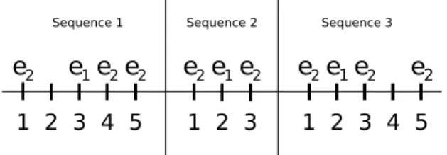
Example:Let us consider the three temporal sequences of Figure 2. S ={S1,S2,S3}. For the pair (e1, e2),O1e1,e2 =
{h(e1, 3), (e2, 1)i, h(e1, 3), (e2, 4)i, h(e1, 3), (e2, 5)i}, O2 e1,e2 =
{h(e1, 2), (e2, 1)i, h(e1, 2), (e2, 3)i} and finally O3 e1,e2 =
{h(e1, 2), (e2, 1)i, h(e1, 2), (e2, 3)i, h(e1, 2), (e2, 5)i}. Additionally, D1
12 ={−2, 1, 2}, D212={−1, 1} and D123 = {−1, 1, 3}. Finally the frequencies of the pair (e1, e2) for each sequence are given by f1
12 = 3, f 2 12 = 2, f 3 12 = 3, hence fmax= 2. 1 2 3 4 5 1 2 3 1 2 3 4 5 Sequence 1 Sequence 2 Sequence 3
e
2e
1e
2e
2e e
2 1e
2e
2e
1e
2e
2Fig. 2. Example of multiple sequences
The roots of the trees for the pair (ei, ej) must hence be such that the number of occurrencesh(ei, ti), (ej, tj)i in all temporal sequences of S is equal to fmax. The following explains how to obtain these roots.
Two sets of supports are considered for each sequenceSk: the set of minimal supports Ik
ij and the set of maximal supports Ikij that guaranty exactly fmaxoccurrences of the pair (ei, ej) in Sk. Whereas minimal supports are used in the algorithm of Cram et al. (2012), maximal supports are a new concept required by our method to deal with multiple sequences. These sets are defined as follows:
Ikij ={I k ij = [t−, t+]|fijk = fmax and∀[t−, t+] ⊆ [t−, t+] fk ij < fmax}. I k ij ={I k ij= [ t − , t+]|fk ij = fmax and∀[t−, t+ ]⊇ [t−, t+] fijk > fmax}.
Example: On the example of Figure 2, the minimal and maximal supports that guaranty exactly fmax = 2 for each sequence are I112 = {[−2, 1], [1, 2]} and I
1 12 = {] − ∞, 1], [−1, +∞[}, I2 12={[−1, 1]} and I 2 12={] − ∞, +∞[}, I312={[−1, 1], [1, 3]} and I 3 12={] − ∞, 2], [1, +∞[}. Then, the minimal and maximal supports obtained for eachSk are combined to obtain all the possibilities for the whole set of sequences S. Let us denote by Icomb
ij and I comb ij the set of minimal and maximal support combinations, respectively: Icombij ={I comb ij ={I 1 ij,· · · , I n ij}|I k ij ∈ I k ij, k = 1,· · · , n}, I comb ij ={I comb ij ={I 1 ij,· · · , I n ij}|I k ij ∈ I k ij, k = 1,· · · , n}. The union of the minimal supports of every combination of Icomb
ij is a candidate for being a tree root for (ei, ej). The set of tree root candidates for (ei, ej) is given by:
RCij={rijα = [ k Ik ij, I k ij ∈ I k ij, k = 1,· · · , n, α = 1, . . . , card(Icombij )}.
However, minimal supports are determined independently for each sequence. As a consequence, a candidate may violate the fmaxoccurrences rule in some of the sequences, in which case it is not valid.
The validity of a candidate can be assessed thanks to the maximal supports. Indeed, the intersection of the maximal supports of every combination of Icombij provides a maximal common interval, denoted M CI, that guaranties exactly fmax occurrences of the pair (ei, ej) in all the sequences Sk∈ S: MCIij ={MCIijβ = \ k Ikij, I k ij ∈ I k ij, k = 1,· · · , n, β = 1, . . . , card(Icombij )}.
Proposition 1. A tree root candidate rα
ijof RCij is valid if ∃β such that rα ij ⊆ MCI β ij, where M CI β ij ∈ MCIij. A valid tree root candidate for (ei, ej) is denoted Rα
ij and the set of such roots is denotedRij. The cardinal of Rij is nij.
Example: Let us build the first following combinations by taking the first elements of the minimal and maximal supports for each sequence: {[−2, 1], [−1, 1], [−1, 1]} ∈ Icomb12 and {] − ∞, 1], ] − ∞, +∞[, ] − ∞, 2]} ∈ I
comb 12 . The intersection of the maximal supports provides a maximal common interval M CI1
12 that validates the union of the minimal supports r112, that is:
r1
12= [−2, 1] ⊆ MCI 1
12=]− ∞, 1].
Hence, a first valid tree root for pair (e1, e2) is given by R1
12 = r121 = [−2, 1]. However, about the second obtained combinations{[−2, 1], [−1, 1], [1, 3]} ∈ Icomb12 and {] − ∞, 1], ] − ∞, +∞[, [1, +∞[} ∈ Icomb12 , the intersection of the maximal supports provides this maximal common interval M CI2
12 = [1, 1] that do not validate the union of the minimal supports r2
12= [−2, 3]. Hence, r212 is not a good candidate to be a tree root, it authorizes 3 occurences in sequences 1 and 3 so it violates the fmax= 2 occurences rule.
The same procedure is applied for f = fmax− 1 and so on until f = 1 to find the tree roots in case no candidate is valid for f + 1 or to find the child nodes of the lower levels of the trees. The lowest level always corresponds to f = 1 and is never empty because the considered pairs have been taken as pairs appearing in all the sequences. The trees for the different pairs (ei, ej) may have a root corresponding to a different frequency. The root frequency for the trees of (ei, ej) is denoted froot
ij . [-2,1] [-1,2] [-2,-1]
e
[1,1] [1,1]e
e
e
e
e
e
e
e
e
1 1 1 1 2 1 2 2 2 2Fig. 3. Set of trees for pair (e1, e2)
Example:For the example of Figure 2, two valid tree roots are found for pair (e1, e2): R1
12= [−2, 1] and R212= [−1, 2]. The set of trees is illustrated in Figure 3 with froot
12 = 2 and n12= 2.
3.2 Chronicle discovery algorithm
Once the constraint database D has been built to account for all the sequences in S as presented in section 3.1, the algorithm for discovering all minimal frequent chronicles for D, given an input frequency threshold fth, is the same as the HCDA algorithm of Cram et al. (2012) but the counting step. This algorithm is hence called HCDA-modified. The counting step is slightly different because we want HCDA-modified to provide all the frequent chroni-cles whose frequency is above the specified threshold. Like in (Cram et al., 2012), the candidate chronicles are called D-chronicles.
The principle of HCDAM is to generate a set of candidate D-chronicles from a chronicle that was proved to be frequent. The set Candidates is initiated with the set of root trees DT. The algorithm maintains two lists:
• the list Frequent includes the candidate D-chronicles that have been proved frequent, i.e. whose frequence is higher or equal to fth, and strictest,
• the list NotFrequent includes the chronicles that have been proved not frequent.
Instead of immediately counting a candidateC, i.e. deter-mining the minimal number of occurences in the sequences of S, the algorithm first makes use of the generality rela-tion and monotonicity property to discard or accept the candidate without counting:
• if there exists a chronicle C0 more general than C in NotFrequent, thenC is not frequent as well,
• if there exists a chronicle C0 stricter than C in Fre-quent, thenC is also frequent.
If none of the two above situations apply, thenC is counted, which is performed with CRS (Chronicle Recognition Sys-tem) (Dousson et al., 1993).
In our algorithm, the candidate is also counted in the second situation to determine its actual frequency, which is necessarily higher than fthand higher than the frequency of the stricter chronicleC0. Obviously, only maximal chron-icles are saved in NotFrequent because this set is used to search for more general chronicles. Conversely, only minimal chronicles are saved in Frequent.
Example: Consider the following sequences of events. Sequence 1 Sequence 2 Sequence 3
(e1, 1.049432) (e1, 13.354919) (e5, 7.207688) (e2, 1.606904) (e1, 14.1784) (e7, 7.36308) (e3, 1.873512) (e3, 14.377672) (e2, 8.00252) (e4, 2.18784) (e4, 14.706472) (e3, 8.273512) (e5, 3.441056) (e5, 15.196873) (e4, 8.482312) (e6, 5.871024) (e6, 18.395527) (e5, 9.8347435)
(e6, 12.974768)
The algorithm HCDA-modified has been used to learn the two following chronicles. The second chronicle is a chronicle of frequency 2, which means that it must be recognized twice to sign the situation captured by the three sequences of the exemple. The first chronicle is the stricter chronicle. It involves the highest set of event with the tightest temporal constraints. It is of frequency 1.
chronicle Chronicle1 { event(e5, t1) event(e2, t2) event(e6, t3) event(e3, t4) t2− t1in [−2, −1] t3− t1in [−1.5, 3.5] t3− t2in [0, 5] t4− t1in [−2, −0.5] t4− t2in [0, 0.5] } chronicle Chronicle2 { event(e5, t1) event(e6, t2) t2− t1 in [−1.5, 3.5] } 4. CONCLUSION
This paper deals with the problem of discovering temporal patterns in the form of chronicles that are common to a set of temporal sequences issued from the same situation. The obtained chronicles then sign the situation and can be used for situation assessment or diagnosis purposes. The paper builds on work by Cram et al. (2012) and extends the proposed algorithm that targets learning the frequent chronicles for one single sequence to multiple temporal sequences that represent variants of a unique situation. This requires to deeply revise the algorithm to generate the constraint database representing the temporal sequences. The revised algorithm is illustrated by a simple example which helps understand the different steps of the method. Future research includes theoretical as well as applied work. The complexity of the modified algorithm, including building the constraint base, should be carefully analyzed and ways to improve efficiency should be studied. On the other hand, it is planned to use this work for a real prognostic problem, applying the algorithm HCDAM to the observable signals of a pressure regulation valve of a modern aircraft in different wear situations.
REFERENCES
Agrawal, R. and Srikant, R. (1994). Fast algorithms for mining association rules. Proc. 20th Int. Conf. on Very Large Data Bases, Santiago, Chile., 487–499.
Carrault, G., Cordier, M.O., Quiniou, R., Garreau, M., Bellanger, J.J., and Bardou, A. (1999). A model-based approach for learning to identify cardiac arrhythmias. In W. Horn, Y. Shahar, G. Lindberg, S. Andreassen, and J. Wyatt (eds.), Proceedings of AIMDM-99 : Artificial Intelligence in Medicine and Medical Decision Making, volume 1620 of LNAI, 165–174. Springer Verlag, Aal-borg, Denmark.
Cordier, M.O., Guillou, X.L., Robin, S., Roz´e, L., and Vidal, T. (2007). Distributed chronicles for on-line diagnosis of web services. In G. Biswas, X. Koutsoukos, and S. Abdelwahed (eds.), 18th International Workshop on Principles of Diagnosis, 37–44.
Cordier, M. and Dousson, C. (2000). Alarm driven mon-itoring based on chronicles. In 4th Sumposium on Fault Detection Supervision and Safety for Technical Processes (SafeProcess), 286–291. Budapest, Hungary. Cram, D., Mathern, B., and Mille, A. (2012). A complete
chronicle discovery approach: application to activity analysis. Expert Systems, 29(4), 321–346.
Dousson, C. and Duong, T.V. (1999). Discovering chroni-cles with numerical time constraints from alarm logs for monitoring dynamic systems. In IJCAI 99: Proceedings of the Sixteenth International Joint Conference on Ar-tificial Intelligence, 620–626. San Francisco, CA, USA. Dousson, C., Gaborit, P., and Ghallab, M. (1993).
Sit-uation recognition: representation and algorithms. In IJCAI: International Joint Conference on Artificial In-telligence, 166–172. Chamb´ery, France.
Fessant, F., Cl´erot, F., and Dousson, C. (2004). Mining of an alarm log to improve the discovery of frequent patterns. Lecture Note on Artificial Intelligence, 3275, 144–152.
Guerraz, B. and Dousson, C. (2004). Chronicles construc-tion starting from the fault model of the system to diagnose. In International Workshop on Principles of Diagnosis (DX04), 51–56. Carcassonne, France. Laborie, P. and Krivine, J.P. (1997). Automatic generation
of chronicles and its application to alarm processing in power distribution systems. In 8th international work-shop of diagnosis (DX97). Mont Saint-Michel, France. Mannila, H., Toivonen, H., and Verkamo, A.I. (1997).
Discovery of frequent episodes in event sequences. Data Mining and Knowledge Discovery, 1, 259–289.
Mitsa, T. (2010). Temporal data mining. CRC Press. Morin, B. and Debar, H. (2003). Correltaion on
intru-sion: an application od chronicles. In 6th International Conference on recent Advances in Intrusion Detection RAID. Pittsburgh, USA.
Pencol´e, Y. and Subias, A. (2009). A chronicle-based diagnosability approach for discrete timed-event sys-tems: Application to web-services. Journal of Universal Computer Science, 15(17), 3246–3272.