Risk Taking of Executives under Different Incentive Contracts: Experimental Evidence

Risk Taking of Executives under Different Incentive Contracts:

Experimental Evidence

Mathieu Lefebvre

University of Liège, CREPP; Boulevard du Rectorat, 7 Bâtiment 31, boîte 39, 4000 Liège, Belgium. E-mail: [email protected]

and

Ferdinand M. Vieider

WZB, Risk & Development Unit, Reichpietschufer 50, 10785 Berlin, Germany. Email: [email protected]

24 September 2013

Abstract

Classic financial agency theory recommends compensation through stock options rather than shares to counteract excessive risk aversion in agents. In a setting where any kind of risk taking is

suboptimal for shareholders, we show that excessive risk taking may occur for one of two reasons: risk preferences or incentives. Even when compensated through restricted company stock,

experimental CEOs take large amounts of excessive risk. This contradicts classical financial theory, but can be explained through risk preferences that are not uniform over the probability and outcome spaces, and in particular, risk seeking for small probability gains and large probability losses. Compensation through options further increases risk taking as expected. We show that this effect is driven mainly by the personal asset position of the experimental CEO, thus having deleterious effects on company performance.

Keywords: executive compensation; risk preferences; experimental finance; prospect theory JEL Classification: D03, G28, G32, J33, L22

#

Financial support from the Agence Nationale de la Recherche (ANR BLAN07-3_185547 “EMIR” project) is gratefully acknowledged. We are indebted to Sylvain Ferriol for programming the experiment, as well as to Marie Claire Villeval, Peter P. Wakker, Klaus Schmidt, Aurélien Baillon and participants at the CREPP seminar, the ESA conference in Copenhagen, and the WISE workshop on experimental economics in Xiamen, China, for helpful comments. All errors remain ours.

1. Introduction

A large part of the performance-contingent pay of executives today is delivered through stock options. Traditionally, the compensation of executives through stock options instead of company shares has been justified by the need of inducing some desirable risk appetite in otherwise risk-averse agents (Agrawal and Mandelker, 1987; Smith and Stulz, 1985). This argument, however, rests on the assumption of global risk aversion by executives (Wiseman and Gomez-Mejia,1998). A wealth of evidence from the empirical literature points in the direction that risk attitudes depend on decision frames and reference points (Baucells et al., 2011; Diecidue and van de Ven, 2008;

Kahneman and Tversky, 1979), and may thus vary over the outcome and probability spaces (Fiegenbaum, 1990; Schmidt and Zank, 2008; Tversky and Kahneman, 1992). Furthermore, the long-standing postulate that linear incentive contracts result in risk aversion on the side of agents lacks empirical evidence. The availability of data on these issues is indeed limited, and often no clear-cut, causal conclusions can be drawn even where such data can be found.

In our experiment, participants are assigned the role of executive of one company. In each period they have to make a choice between two investment options to invest total company assets: a high volatility investment and a low volatility investment. By design, the high volatility investment is always inferior in terms of expected value in order to test whether excessive risk taking will occur. Our results indicate that excessive risk taking can be generated by both preferences and incentives. Under linear compensation through long-term stock-ownership, which has traditionally been hypothesized to result in excessive risk aversion, we find high levels of suboptimal risk taking. This is mostly due to risk preferences, and can to a large extent be explained by non-linear

probability weights. When incentives for risk taking are created under the form of compensation through options, these incentives show an effect on top of the preferences just described. They thus increase suboptimal risk taking, an effect that is mainly driven by options that cannot be exercised because the price at which they allow to buy stock lies above the current share price. Both

preferences and incentives thus result in lower company performance. The decline in company performance caused by incentives, however, is larger than the decline caused by preferences, which can be traced back to the drivers of behavior in the different payoff regimes.

Experiments have the advantage of permitting controlled variations in one independent variable at the time, thus permitting the isolation of clear causal relationships. Experiments are increasingly common in finance for issues that are difficult to disentangle in the real world (e.g. Fellner and Sutter, 2009; Fox et al., 1995; Gneezy and Potters, 1997; Sutter et al., 2011), and can significantly supplement results obtained from the analysis of real-world data.Furthermore, experimental investigation makes simplifications aimed at isolating fundamental causal

relationships, which closely resemble the simplifications made by theoretical models. The present paper proceeds as follows. Section 2 presents a discussion of different compensation schemes and develops a simple model predicting choices based on different

theoretical assumptions. Section 3 presents the experiment and its main results. Section 4 discusses these results, and section 5 concludes the paper.

2. Compensation schemes and investment behavior

2.1 Stock option compensation versus stock compensation

The importance of stock-option payments has increased dramatically over the last two or three decades and holds a prominent place in the overall compensation of executives (Core et al. 2003; Hall and Liebman, 1998). Traditionally, compensation through stock options has been explained as a solution to the agency problem inasmuch as it counteracts the natural risk aversion of executives (Agrawal and Mandelker, 1987; Feltham and Wu, 2001; Guay, 1999; Hall and Liebman, 1998; Smith and Stulz, 1985). Options shelter executives from potential losses since they do not have to be exercised in case of a decline in stock prices (Bebchuck and Fried, 2003; De Fusco et al., 1990). The result that stock options may increase risk taking when the latter is desirable is thus well established. It is less clear what will happen when any such risk taking is undesirable.

It is also generally accepted that paying executives in restricted company stock reduces risk taking by increasing the linearity of the incentive instrument (Holden, 2005; Jensen and Murphy, 1990). Traditionally, this has mostly been seen as undesirable, since it may trigger risk aversion on the side of executives, which is undesirable from the point of view of a risk neutral investor. There is, however, a lack of empirical evidence on this point, and the conclusion holds true only as long as one assumes that executives maximize expected utility with a concave utility function, i.e. they are risk averse over the whole probability space. People's risk attitudes have, however been found to vary widely over the probability and outcome space (Abdellaoui, 2000; Mezias, 1988; Piron and Smith, 1995; Wu and Gonzalez, 1996)—a finding that has also been shown to hold for large firms (Chou at al., 2009; Fiegenbaum, 1990). In the following we thus adopt prospect theory as a

descriptive theory of choice (Tversky and Kahneman 1992). Prospect theory is increasingly used to explain issues in finance that were previously considered paradoxical (e.g., Bernartzi and Thaler, 1995; Fellner and Sutter, 2009; Gneezy and Potters, 1997; Weber and Camerer, 1998). It has been found to hold not only for students, but also for the general population (Booij et al., 2010) and influence the behavior of professional traders (Abdellaoui et al., 2013; Haigh and List, 2005) and executives (List and Mason, 2010).

2.2 A simple model and some initial hypotheses

In this section we develop a model aimed at generating hypotheses for our empirical investigation. Although it easily generalizes to a wider class of compensation schemes, we will adopt the

terminology of our experimental investigation to simplify exposition. Executives choose between investing into a low volatility (LV) investment project or a high volatility investment (HV) project. The expected value (EV) of the high volatility investment opportunity is always inferior to the one of the low volatility investment by design (EVHV<EVLV), since we want to test the conditions under which risk taking by executives may be excessive. As implicit in the designation, the standard deviation of the high volatility investment is always larger than the one of the low volatility investment: σHV > σLV .

In each period, the experimental CEO has to make a choice between two investments. Such choices are repeated for T periods. Experimental CEOs are compensated either through stock options or company shares. Under stock ownership, the experimental CEO is compensated through shares in the firm she manages that are not tradable until the end of the contract, T. Under a stock-option contract, the executive receives, each period, a grant of stock stock-options that become vested in the subsequent period, so that they can be exercised in any period until the end of the contract at T. These stock options are emitted at-the-money at the exercise price et =st, where st represents the

value of shares at the time t when the options are emitted (i.e., giving the right to buy stock for the price at the time of their emission). 1 For simplicity we will assume that whenever an option is exercised, the shares thus called will be resold immediately, so that realized gains for options emitted at time t and sold at time i will be si–et, s > e and i > t, which imposes that options can be only sold after their emission period.

In this section we model ways in which experimental CEOs may take excessive risks from the point of view of the shareholders. Such increased risk taking may take place through one of two mechanisms: 1) a preference for risk taking; or 2) incentives for risk taking. The case of preferences is most clearly made under compensation through stock, since different theories about preferences yield similar predictions for compensation through options (this will be addressed when discussing incentive effects below). This is also why the case of compensation through options is ideal to filter out the effect of incentives for risk taking. We address the two explanations in turn.

1 _{An option is said to be at-the-money when it gives the right to buy stock at exactly its current market value, ie. no}

profit could be made by exercising the option and buying the stock and reselling it immediately (joint buying and selling is assumed throughout). Similarly, an option is said to be in-the-money when it gives the right to acquire stock at below current market value, ie. can be exercised at a profit; and out-of-the-money when the buying price is above current market prices.

Linear compensation and preferences for risk taking

Under linear compensation through company stock, a uniformly risk averse or risk neutral

experimental CEO has no reason to choose the HV investment in our experimental setting.2 Since decision makers may, however, not be uniformly risk averse or risk seeking over the probability and outcome spaces, we adopt prospect theory as our descriptive theory of choice (Kahneman and Tversky, 1979; Tversky and Kahneman, 1992). One of the most important innovations of prospect theory is reference dependence—the idea that the evaluation of a given prospect or outcome

depends on a reference point adopted by a subject. Reference dependence may give rise to different risk attitudes for gains versus losses as well as to loss aversion, a phenomenon by which people attribute more weight to losses than to monetarily equivalent gains (Bleichrodt et al., 2009;

Köbberling and Wakker, 2005). Under prospect theory, attitudes towards probabilities are expressed by probability weighting functions, while the utility function expresses attitudes towards outcomes. The prospect value (PV) of a binary prospect ζ that provides monetary outcome x > 0 with a

probability p and the monetary outcome y < 0 with a complementary probability 1–p can thus be written as:

PV(ζ)=w+(p)*U(x) –λ*w–(1-p)U(y), (1)

where w+ indicates probability weighting for gains, w– probability weighting for losses, U(x) is taken to be utility over monetary gains x, and U(–y)= –λ*U(y) is the utility over monetary losses, where λ is the loss aversion parameter. We will also designate gain percentages by α and loss percentages by β, so that for instance a gain in share value from a LV investment at time i can be written as αLV*si,where si indicates the share price in period i. This experimental focus on changes relative to current company value makes this value salient, and we thus adopt the status quo as the reference point throughout. Typical prospect theory estimates predict people to be risk averse for moderate to large probability gains and small probability losses; and risk seeking for moderate to large probability losses and small probability gains. Nevertheless, such patterns mask considerable differences at the individual level (Abdellaoui et al., 2011). In our empirical analysis we will thus rely on individual level measurements rather than typical aggregate patterns.

We can now represent the decision problem under stock compensation. The problem is

2

An agent is defined as risk averse whenever she weakly prefers the expected value of a prospect over the prospect itself. Similarly, she is defined as risk seeking whenever she weakly prefers the prospect over its mathematical

expectation. Finally, she will be risk neutral if she is both risk averse and risk seeking (Segal and Spivak, 1990; Wakker, 2010). Notice also that since we are using only two-outcome prospects, different definitions of risk aversion will actually yield the same conclusions.

identical for all periods by design, so that we can look at one period in isolation. Assuming that the current stock value or status quo acts as a reference point, a CEO will thus choose the LV

investment whenever

w+(pLV)*U(αLV*si) – λ*w–(1–pLV)*U(βLV*si) > w+(pHV)*U(αHV*si) – λ*w–(1–pHV)*U(βHV*si), (2)

where p represents the probability of a successful investment. Typical prospect theory functionals observed on average, such as risk seeking for small probability gains and for losses, now allow us to derive some predictions on average behavior. The measurements obtained of individual preferences, furthermore, will allow us to test whether individual differences matter for behavior, thus isolating the causal effects. We hypothesize that:

H1: Under stock ownership, we will not observe universal risk aversion as predicted by

classical financial theory. Risk taking will be observed whenever a) subjects are risk seeking for small probability gains, so that the generally smaller probabilities of winning in the HV investment are overweighed relative to the generally larger probabilities of winning in the LV investment; b) subjects are risk seeking for losses, so that the relatively large probabilities of losing in the HV investment are underweighted relatively to the smaller probabilities in LV; and c) subjects display low levels of loss aversion.

Incentives effects and compensation through stock options

When an experimental CEO is compensated through options, then her compensation varies linearly with the firm’s share price only to the extent that the share price exceeds the exercise price of the option, and indeed to the extent that all investment outcomes keep the option in- or at-the-money. We will now try and highlight the effect of option compensation by comparing it to the previous case of stock compensation. In order to do that, we will again adopt prospect theory to model choices. We start by looking at the problem in period zero, or whenever all previously emitted stock options have been sold, and when a CEO thus holds only stock options which are at-the-money. An experimental CEO will now choose the HV investment over the LV investment if

w+(pHV)*U(αHV*si) > w+(pLV)*U(αLV*si) (3)

Notice how equation 3 can be directly derived from equation 2 by dropping the part concerning losses. This derives from the fact that while any increase in stock value can be cashed in, decreases in stock value do not result in monetary losses since options will not be exercised. Although there may still be a loss in future earning potential given a stronger decrease in share price from a HV

investment, this effect is likely to be secondary and the attention will be mostly focused on the gain side of the prospects. Some of the preference factors, on the other hand, will remain the same: choices of the HV investment will again be reinforced by commonly found overweighting of small probabilities (Abdellaoui et al., 2011; Wu and Gonzalez, 1996), given that the probability of a success is generally lower in the HV investment than in the LV investment.

Let us now take the case in which in addition to the options just emitted, the CEO holds one additional option bundle, which is either in-the-money or out-of-the-money. Since one of the option bundles (the one just emitted) will always be at-the-money, equation 3 will still be relevant for the decision. In addition, however, for options that are in-the-money there is now the consideration that any currently existing value, si-et, may be lost (either completely or in part, depending on the value of βHV relative to βLV). Loss aversion over accumulated value will thus work against the risk-seeking tendency produced by newly emitted options. If, on the other hand, the additional option bundle is out-of-the-money, this will create additional incentives for risk seeking in order to push the share price above the exercising value of the currently out-of-the-money options. The exercise price of that bundle will thus act as an aspiration level (Carpenter, 2000; Diecidue and van de Ven, 2008; March, 1988). This risk-seeking tendency is further reinforced by the fact that no losses can be felt for options that are at- or out-of-the-money, so that loss aversion will not play a role for the

decision. This intuition leads us to the formulation of the following hypothesis:

H2: Under stock option compensation, executives will display a higher propensity for risk

taking than under compensation through stock since they are sheltered from losses and look mainly at the gain part; a) subjects will be particularly risk seeking if all the options held at the moment of the decision are out-of-the-money; b) subjects will be more reluctant to take risks if all options currently held are in-the-money;

Please notice how hypotheses H2a–b are not unique to prospect theory. Similar arguments can indeed be made based on the cutoff of lower tails at the emission value of an option in an expected utility calculation. The question here is rather to what extent options increase risk taking relative to compensation through stock. No direct evidence exists on this point.

3. The Experiment 3.1 Experimental Design

Subjects. 96 subjects were recruited from a list of experimental subjects maintained at GATE, University of Lyon, France, using the ORSEE software (Greiner, 2004). Groups of six subjects needed to be formed, so that all sessions were run with either 12 or 18 subjects each. Subjects had

an average age of 22 years (standard deviation 4.96 years), and 55% of subjects were female. 63% were studying economics or business management, 31% mathematics or engineering and the rest did not specify their study major.

Main Task. In the main part of the experiment, groups of six subjects are formed. The composition of the groups is kept fixed for the 15 periods, and subjects do not know whom they are matched with. At the outset of the experiment, each group member is assigned the role of CEO of one company. In their function of CEO of a company, subjects are confronted with a sequence of investment decisions over 15 periods. In each period, the experimental CEO decides between two investment opportunities into which to invest the total stock of company assets (screenshots in appendix A). The initial stock value of the company is €100 ($150) for everyone, this corresponds to 100 shares of €1. The final value of the company will be determined by the outcome of the 15 investment decisions.3 At the same time, each group member also acts as shareholder in the five other companies managed by the five other subjects in her group. The shareholder role is a passive role, in the sense that it does not require any action on the part for the subject.4 However, it

contributes towards final payoffs as follows. Each subject is given one share with the initial value of €1 ($1.50) in each of the other five companies in her group. She is then paid the final value of that share (total company value divided by 100) at the end of the 15 periods. Each CEO observes only the performance of her own company for the 15 periods of the experiment, and receives feedback about the success of her own investment after each period. The performance of other companies the experimental CEO is a shareholder in is not observed at any time during the experiment. Earnings from the shareholder function can thus not be used to hedge any risks, since they are neither known nor can be influenced. The experiment was conducted using REGATE (Zeiliger, 2000).

Investment Decisions. In each period, the CEO has to choose between two investment opportunities in which to invest total company assets. The investment opportunities are described in terms of percentage increases or decreases of the company’s value. Investments are displayed graphically by means of pie charts representing the probabilities of winning and losing in addition to a verbal description. The choice is always between a high volatility (HV) and a low volatility (LV) prospect.

3

Please note that any change in share prices in our experimental model are generated purely by changes in the underlying value of the company assets as determined by investment outcomes—there is no market for shares.

4_{We decided to add shareholders for two reasons. One is that subjects may decide differently when responsible for}

somebody else as well as themselves (Charness and Jackson, 2009; Pahlke, Strasser, and Vieider, 2011), so that this design element was needed to add realism to the setup. The second is that we also wanted to test for the effect of increased accountability towards shareholders, the effects of which are reported elsewhere (Lefebvre and Vieider, 2013).

The LV prospect always offers a higher expected value than the HV prospect, so that any risk taking observed is excessive from the point of view of the company or the shareholders by definition, inasmuch as it delivers a lower expected value. Indeed, differences in expected value were such that consistently investing in the LV option would yield an expected final company value that was almost 30 percentage points higher than the one obtainable by consistently investing into the HV option. In the initial instructions, subjects were given a graphical overview of the general

characteristics of the two investments as well as an example representing a choice between two 'typical investments'. This graphical display, as well as the instructions and a table showing the parameters of all prospect pairs can be found in the appendix B.

Stock-Ownership Condition. In the stock-ownership condition subjects obtain an initial endowment of 10% of the company stock, corresponding to an initial value of €10 ($15). At the end of the 15 periods, they are paid the final value of their shares. They cannot sell their stock before the end of the 15 periods. Their payment structure thus coincides with the one of shareholders, who also obtain the value of their shares at the end of the 15 periods. The compensation parameters were designed in such a way that the total amount to be earned on average should be roughly equal to the

compensation in the stock-option condition.

Stock-Option Compensation. Each CEO obtains five stock options in each period, which are emitted at-the-money, i.e. giving the right to buy company stock at the current stock value. For example, the five options granted before period 1 investment decisions are made give each the right to buy one share of the company at €1 ($1.50). The options get vested in the subsequent period and remain exercisable until the end of the game, so that they can be 'cashed' at any time. While in reality the options give right to buy company stock, which can then be either sold or kept, this decision was unified for simplicity. That is, exercising options in the experiment means buying stock and reselling it immediately, thus realizing the difference between current stock value and the exercise price of the option. This process closely mimics real-world practices of “cashless exercise” (Heath, Huddart, and Lang, 1999). Thus, in every period after the first, the CEO is called upon to decide whether to cash her options after the results of the investment have become known (separately for options emitted in different periods). She will then obtain the new options and decide which investment to take for the subsequent period.5

5 _{The exercising decisions themselves are not analyzed in this paper, since we are purely interested in the incentive}

Risk attitudes. We used the method of Abdellaoui et al. (2008) to elicit detailed risk attitudes. Risk attitudes were elicited at the outset of the experiment, before any treatments were introduced. We elicited six certainty equivalents for pure gain prospects, six for pure loss prospects, and one for a mixed prospect. This allows us to derive probability weighting functions for gains and losses, and loss aversion. While one choice was selected for real pay in each domain (gains, losses, and mixed gambles), no information on payoffs was given until the very end of the experiment to avoid income effects. A detailed description of the risk attitudes can be found in appendix D.

3.2 Results: Risk taking and company performance under alternative compensation regimes

Fig. 1. Average choice of HV investment in the option treatment (OP) and the stock ownership treatment (ST)

Figure 1 summarizes choice behavior over the 15 investment periods. Subjects compensated through stocks take significant amounts of risk (38.2% of the time on average). This contradicts accounts according to which linear compensation will yield excessive risk aversion, confirming H1. Subjects compensated through options chose the inferior high volatility investment on average 48.8% of the time. This is significantly more often than under stock compensation, showing clearly the effects of incentives (z=1.98, p<0.05, two-sided Mann-Whitney test over the sum of risky

.2 .3 .4 .5 .6 .7 % o f ri sk y ch o ice 1 2 3 4 5 6 7 8 9 10 11 12 13 14 15 Period OP ST

choices), and thus confirms H2.

This is also reflected in company performance. Figure 2 shows the development of mean stock values by compensation type. It can clearly be seen that the mean stock value of companies managed by CEOs compensated through stock outperforms companies managed by CEOs compensated through stock options. Indeed, the mean final value after 15 periods of companies managed by CEOs compensated through stock is about 11 percentage points higher than the mean final value of companies managed by CEOs compensated through options. Nevertheless, the company performance obtained under stock compensation still falls short of the simulated performance under the assumption that the superior LV investment had been taking in all periods (which effectively corresponds to the EV of the prospect being realized in each period). The effect here is somewhat less strong, with final performance in the payoff relevant period only about 7 percentage points short of the expected final value. This is partially due to luck in intermediate periods, and partially to particular choice patterns that we will analyze in more detail in the next section.

Figure 2: Average stock evolution in the option (OP) versus stock ownership (ST) treatment over the 15 periods.

3.3 Individual risk preferences and investment under stock ownership

1 0 0 1 1 0 1 2 0 1 3 0 1 4 0 Me a n va lu e o f st o ck 1 2 3 4 5 6 7 8 9 10 11 12 13 14 15 Period OP ST Simulated

We next look at whether we can explain choice patterns under compensation through stock. Table 1 shows the results of a random effects Probit regression for the stock ownership condition. The marginal effects of changes in explanatory variables are presented.The dependent variable is the choice of the HV investment. Specification (1) shows the regression controlling only for

demographics and the difference in expected value between the LV and HV investment. This establishes a baseline, showing that the difference in expected value between the LV and the HV investment plays an important role, with risk taking decreasing in this difference as we may expect. This result also goes some ways towards explaining why company performance is not too bad notwithstanding the high levels of risk taking, since risk taking is most frequent when HV is not much worse than LV in terms of expected value. We find that risk taking declines with age, which is quite typical; however, we also find that males are less risk loving than females, which goes against the prevalent finding in the literature (Charness and Gneezy, 2012), once we control for probability weighting.

Table 1: Risk attitudes in the stock-ownership condition (random-effect probit model, marginal effects) Dep. Variable: choice of the risky

investment

(1) (2)

(3)

Difference in expected value (normalized: average=0) -0.146** (0.062) -0.154** (0.062) -0.152** (0.061) Risk seeking for small gain

probabilities (CE/EV|p=0.1)

0.192*** (0.054)

0.187*** (0.051) Risk seeking for large loss

probabilities (–(CE/EV) |p=0.7) 0.416*** (0.159) 0.428*** (0.154) Loss aversion -0.016 (0.010) Male -0.067 (0.074) -0.191*** (0.067) -0.198*** (0.065) Age -0.014** (0.006) -0.021*** (0.006) -0.022*** (0.005) Economics major -0.164** (0.075) -0.177*** (0.061) -0.201*** (0.061) Constant -0.825** (0.345) -0.199* (0.593) -0.012 (0.587)

Nb observations 720 (48 subjects) 720 (48 subjects) 720 (48 subjects)

LL -421 -411 -410

Note: *** significant at the 1% level; ** at the 5% level and * at the 10% level. Standard errors in parentheses.

to be theoretically relevant. A likelihood ratio test shows that adding these preference measures significantly increases the explanatory power of the model (χ2(2)=45.33, p<0.001). We use the ratio of the certainty equivalent (CE) elicited for the prospect giving a 10% chance to obtain €20 or else nothing to its expected value (EV) as a measure of the extent to which small probabilities are overweighed (CE/EV>1) or underweighted (CE/EV<1). The coefficient of this variable is indeed positive and highly significant, showing that subjects who overweight small probabilities take the HV investment significantly more often. This confirms our hypothesis H1a. Furthermore, we also find a strong effect of the extent to which large loss probabilities are underweighted (measured as –(CE/EV) elicited for a prospect with a 70% probability of losing €20 or nothing), confirming our hypothesis H1b. The latter two effects are displayed in figure 3. Adding loss aversion in

specification (3), however, does not add any explanatory power to the model. Loss aversion is not a significant predictor of choice, rejecting H1c.

Figure 3: The effect of individual risk attitudes on risk taking

Note: The weighting of small probability is obtained by the ratio of the certainty equivalent elicited for the prospect giving a 10% chance to obtain €20 or else nothing to its expected value. We classified a subject as risk seeking for losses if she was risk seeking for at least 4 out of 6 prospects in the loss domain (see appendix D).

3.4 Incentivizing risk taking through stock options

We next take a closer look at H2. Figure 4 displays levels of choices of the HV investment in the option treatment, separated by asset position and by overweighting of small probabilities. This allows us to single out the drivers behind the increased risk taking observed under option

compensation. The basic level of risk taking when all options are at-the-money (42% on average) is virtually identical to the level of risk taking observed when executives hold a mixed bundle

33% 52% 30% 42% 0% 10% 20% 30% 40% 50% 60%

Risk seeking for loss Not risk seeking for loss

containing both options that are in- and out-of-the-money (41%). Choices of the HV investment are reduced when CEOs hold only options that are in-the-money (29%). The most striking change, however, occurs when all the options held are out-of-the-money. In this case, subjects choose the HV investment much more often—on average 72% of the time. Indeed, if we lump together the three cases of options being in-the-money, at-the-money, and the mixed case, the average risk taking of 39% is very similar to the one observed under compensation through stock. It is the case of options being out-of-the-money to drive the additional risk taking we observe under

compensation through options compared to compensation through stocks.

Figure 4: risky choices by asset position and weighting of small probabilities

Note: The weighting of small probability is obtained as the ratio of the certainty equivalent elicited for the prospect giving a 10% chance to obtain €20 or else nothing to its expected value.

Table 2 tests H2 statistically through a random effects Probit regression. Specification (1) shows that the difference in expected value between the HV and the LV investment now plays no longer a role in explaining choices. To test our hypotheses H2a and H2b, we need to separate the options held by the CEO into clear-cut categories. To this end, in regression (2) we introduce two dummies indicating that all options held are in-the-money or out-of-the-money6, with the effect being

measured against the case in which the CEO holds either only options which are at-the-money, or a mix of options, some of which are in- and some out-of-the-money. Adding asset positions

significantly improves the explanatory power of the model (χ2

(2)=53.24, p<0.001). Holding only options that are in-the-money significantly reduces risk taking, thus confirming H2b. When all options held are out-of-the-money, on the other hand, risk taking increases considerably. This

6

The bundle just emitted is always at-the-money by definition, so that it will be disregarded for the creation of the “all in-the-money” and “all out-of-the-money” categories. When the only options held are the ones that have just been emitted, then this will be categorized as a case of “all at-the-money”.

36% 50% 35% 51% 25% 35% 76% 69% 0% 10% 20% 30% 40% 50% 60% 70% 80% 90%

All-at-the-money Mixed All-in-the-money All-out-the-money

confirms H2a.

In specification (3) it is shown that adding the usual measure for overweighting of small probabilities does not increase explanatory power (χ2(1)=1.01, p=0.314). Specification (4) adds interaction terms of overweighting of small probabilities with the asset position dummies, which does improve model fit (χ2

(2)=6.42, p=0.040). The simple effect of the overweighting term now captures the effect of risk seeking for small probabilities when all options are at-the-money or the experimental CEO holds a mix of options. It shows that in this case, probability weighting is indeed relevant. It is also not significantly different from this effect when all options are in-the-money. This shows that in these situations, preferences do matter in a fashion that is analogous to the one

observed for stock. The interaction with the dummy indicating that all options held are out-of-the-money, on the other hand, is significantly negative. Indeed, here the preferences seen above are overwhelmed by the incentive to take risks created by the compensation through stock options.

Table 2: Risk attitudes in the stock-options condition (random-effect Probit model, marginal effects)

Dep. Variable: choice of the

risky investment (1) (2) (3) (4)

Difference in expected value -0.075 (0.066) -0.092 (0.067) -0.096 (0.067) -0.101 (0.067) Options mixed or

at-the-money Ref. Ref. Ref.

All options in-the-money -0.154** (0.063)

-0.154** (0.064)

-0.033 (0.152)

All options out-the-money 0.301*** (0.047)

0.299*** (0.048)

0.533*** (0.089) Risk seeking for small

probabilities (CE/EV|p=0.1)

0.069 (0.068)

0.145* (0.075) All options in-the-money *

risk seeking small p

-0.104 (0.113) All options out-the-money *

risk seeking small p

-0.223** (0.089) Male 0.066 (0.086) 0.043 (0.080) 0.030 (0.080) 0.029 (0.079) Age 0.013 (0.012) 0.013 (0.012) 0.013 (0.011) 0.014 (0.011) Economics studies -0.022 (0.097) -0.047 (0.089) -0.067 (0.091) -0.062 (0.091) Constant -0.669* (0.367) -0.626* (0.356) -0.788** (0.389) -1.058*** (0.406)

LL -434 –407 -407 -404

Note: All specifications include period effects and control for gender, age and field of study.*** significant at the 1% level; ** at the 5% level and * at the 10% level. Standard errors in parentheses.

4. Discussion and conclusion

We find that compensating executives through restricted company stock does not result in uniform risk aversion, as predicted by classical financial theory. Quite to the contrary, risk taking under stock compensation is substantial. Our prospect-theory-based model explains such choices quite well. Individual preferences, mostly under the form of non-linear probability weights, are found to have considerable explanatory power. To the best of our knowledge, this use made of individual risk attitudes is quite unique in the literature and may constitute a promising approach for future

investigations. A bit less surprising, though still important, is that incentives provided through stock options increase risk taking even when the latter is excessive for the shareholders. Current asset holdings strongly influence choice behavior. This is especially true when all options held are out-of-the-money, which we have seen to drive almost the whole increase in risk taking under

compensation through options.Given that the effect of incentives is determined mostly by the personal asset position of the experimental CEO rather than by considerations pertaining to company value in general, company performance is reduced considerably by incentives to take risks. Risk taking due to experimental CEO’s risk preferences under stock compensation does also depress company performance. However, since incentives of shareholders and experimental CEOs are aligned in this case, choices take differences in expected value between the investment

opportunities into account, and thus have a less deleterious effect on company performance. One important criticism that could be brought against our results is that, by using relatively low stakes, it underestimates risk aversion. Given that under prospect theory risk attitudes are determined by a combination of probability weighting, utility curvature, and loss aversion, a very concave utility function for gains may well counteract the probability weighting we have found to drive results. Notice, however, how the typically convex utility function in the loss domain may actually increase risk seeking when decisions take place in the loss domain. Taken together, this does not show a clear direction in which decisions might change. Existing studies from the management literature do indeed indicate that the typical pattern of risk attitudes predicted by prospect theory persist for large-scale decisions (Fiegenbaum, 1990; Jegers, 1991).

The nature of the compensation scheme is not the only difference between our option and stock-ownership treatments. One characteristic of the stock-ownership plan that seems rather fundamental is the long-term nature of the stock compensation, which is contrasted to the

short-term structure of option compensation. In reality, stock-ownership often provides short-short-term incentives as well, and may in such a case produce investment behavior that is closer to the one observed for options (Bebchuk, Cohen, and Spamann, 2009). Given the main purpose of our study—testing whether the prediction of zero risk tolerance under linear compensation contracts stands the empirical test—a longer time horizon such as the one implemented in our experiment does indeed constitute a stronger test. Any excessive risk taking that we have found can thus be expected to increase under shorter-term compensation structures.

There is, however, also an opposite case to be made—that increasing the vesting periods of options may reduce risk taking. This, however, may or may not be true. The evidence from our experiment points in the direction that risk taking under option compensation strongly depends on asset positions. This in turn indicates that risk taking under longer vesting periods may well decrease as long as any options held are in-the-money. If, on the other hand, they should be out-of-the-money after a decrease in stock prices, longer vesting periods may increase risk taking even when such risk taking is sub-optimal for the shareholders. The exact effect will thus depend on the specific circumstances and is ultimately an empirical question.

Obviously, the experimental environment we use to study the problem is highly stylized. In reality, executives' decisions are likely to be influenced by a host of other factors, and incentives exert an influence not only through current compensation mechanisms but also through long-term career concerns (Holström, 1999). Nevertheless, we think that our experimental environment captures the essentials of the problem quite well. To the extent that classical theory predicts

compensation through restricted company stock to result in excessive risk aversion, this prediction should hold in our experiment. Not only do we not find any excessive risk aversion—we even find levels of risk taking that are excessive for the shareholders and the company.

At this point, we also need to address potential subject pool effects. It is often alleged that using students as experimental subjects may reduce the external validity of any results obtained. The fact that the overwhelming proportion of our subjects are economics and business students from French elite schools—and that future CEOs can be expected to be drawn from that pool to a large extent—seems to reduce such concerns. Furthermore, alleged subject pool effects need not always go in the expected direction. For instance, Haigh and List (2005) found that myopic loss aversion is actually accentuated by using professional traders instead of students in an

experiment—the opposite of what the authors had expected. This goes to show that one ought to be careful when making assumptions about subject pool effects—and that having more experience with the kind of decisions subjects are called upon to take in our experiment may just as

as the opposite effect.

Appendix A: Decision Screens, Main Experiment i) Investment screen

Appendix B: Instructions experiment (option treatment)

Thank you for participating in this experiment in decision making! The present experiment consists of two parts. The instructions for part 1 are included hereafter. The instructions for part 2 will be distributed once everybody has completed part 1. You will be compensated with whatever you earn during the experiment according to the procedures described in the instructions.

The instructions for part 1 will be read to you shortly. Please do not hesitate to ask if you have any doubts. Also, you can consult these instructions at any time in case you should not understand something. If you should still have questions during the experiment, please raise your hand and an experimenter will come and assist you.

Please consider each decision carefully. Take a careful look at outcomes, signs of these outcomes, and the probabilities associated to them before taking a decision. Please feel free to use these instructions for notes at any time—a pen is provided on your table. Remember that your final payoffs from this experiment will depend crucially on the decisions you make (and of course, on chance).

Good luck!

Instructions part 1

Part 1 of the experiment consists in choices between lotteries. All the choices you make are

completely confidential and cannot be traced back to you personally. Please consider each decision

problem carefully before you indicate your decision, as your final payoff will depend on your choices in addition to chance.

In the choice pairs involved in part 1, you will be called upon to make repeated choices between a sure amount of money and a lottery with two outcomes. As to the outcomes of the lottery, there are three basic types of lotteries: 1) lotteries giving you a certain probability to win an amount of money, and a complementary probability of winning nothing (pure gain lottery); 2) lotteries giving you a certain probability to lose an amount of money, and a complementary probability of losing nothing (pure loss lottery); and 3) lotteries giving you a probability of winning a certain amount of money and a complementary probability of losing a certain amount of money (mixed lottery). All

the information necessary for you to take a decision will be displayed on the computer screen. Given this setup of the lotteries, and given that the parameters of a decision change for each decision problem that is presented to you, it is crucial that you pay close attention to both

outcomes and probabilities. Also, pay attention to the sign of the outcome as it may be positive or

negative! While you can incur losses in this part of the experiment, the payoffs are calibrated in such a way that it is extremely unlikely for you to lose money over the course of the whole experiment.

For pure gain or pure loss lotteries, you will be asked to choose repeatedly between any given lottery and different certain amounts. According to your choices, the certain amount will be adjusted upwards or downwards for the subsequent decision. You will then be asked again to choose between the new certain amount and the lottery. After five choices, you will pass on to the next lottery. For mixed lotteries, a procedure analogous to the one described above is used. The only difference is that for these lotteries what changes in subsequent iterations is not the sure amount of money (which now stays always at 0), but rather the amount to be lost in the lottery. Below you find an example of a choice for a pure gain lottery and for a mixed lottery.

We next describe how your payoffs for this part of the experiment will be determined. Only some of the choices you make will be randomly drawn and played for real money. While the exact procedure is described in detail below, the most important thing for you to know is that you will perform best

if you make each decision as if it were the only one to be played for real. In other words, there

does not exist any way in which you can outsmart the system by choosing according to some predetermined strategy.

Three choices will be extracted for real play from the lotteries presented to you in part 1—one choice involving a pure gain lottery, one choice involving a mixed lottery, and one choice involving a pure loss lottery. All choices within the given domain have the same probability of being

extracted.

Whatever choices are extracted will then be played out at the end of the experiment. If in the choice that is extracted you have chosen the sure amount, that amount will be added to (or subtracted from for loss lotteries) your total payoff. If you have chosen the lottery, a random draw will determine whether you have won or lost, and the corresponding amount will be added or subtracted from your total payoffs.

The payoff will only be determined once the whole experiment is finished. When you are done with the questions in part 1, please wait for the other people in the experiment to finish as well. As soon as everybody has completed the first part, we will proceed to distributing the instructions for part 2.

Instructions part 2 [distributed after part 1 was done; option treatment]

In this part of the experiment you will be asked to take repeated decisions over 15 rounds. You have

two roles in this part, one as CEO of a company, and one as stockholder in 5 other companies

managed by five other people in your group. Groups are randomly formed at the beginning of part 2 and stay the same for all 15 rounds. Just as you are a shareholder in the 5 companies managed by the other 5 people in your group, the other 5 people in your group are shareholders in your company and part of their payoff thus depends on your company's performance.

Please notice that your decisions are completely anonymous, and that neither the experimenter nor any of the shareholders in your company (the other 5 people in your group) can trace any decisions or outcomes back to you. As a matter of fact, neither you nor the other people taking part in the experiment will know who of the others in the experiment was in their group of 6.

In your function as CEO, you are managing a company. Your company has an initial value of 100

euros, corresponding to 100 shares of the value of 1 euro each. Your main decision will be to choose in each period which of two investment projects you want to invest the assets of your company

in: investment A or investment B. You will have to make a choice between these two options, and

you have to invest the total value of your company in every period. Each investment will be described for each period, and is characterized by its outcomes and its probabilities. Outcomes are given in percentage changes of company value, which can be either positive, negative or zero.

Example:

A typical choice is shown in the screen below. In the example shown, you are called upon to decide between two investments for your company assets:

- investment A, which gives you a 50% chance that the company assets will increase by 8% and a 50% chance that they will decrease by 4%

- investment B, which gives you a 20% chance that the company assets will increase by 40%, and an 80% chance that the value of your company assets will decrease by 8%

Imagine that you are facing the first investment decision (period 1), and that the company you manage is thus worth 100 euros. Imagine now you choose investment A and your investment is successful. Your company is now worth 108 euros, which corresponds to a value of 1.08 euros per

share. This will be your starting value for period 2. There are 15 periods of investment in total.

Payoffs:

Contrary to part 1, all your decisions will now count towards your final payoff. Your payoffs are determined as follows. Before each investment period, you will obtain 5 stock options that give

you the right to buy company stock in any future period for the exercise price indicated on the option. Options will be emitted at company value and will become vested (that is, cashable) in the subsequent period. You can then decide separately for options obtained in different periods whether you want to: 1) cash the options, thus obtaining the difference between the current stock price and the emission value of the option (times 5 since you have five options); or 2) keep the options and preserve the right to exercise them in a later period.

Example (continued):

Following the example given above, this means that before your first investment decision you have obtained 5 stock options with an exercise price of 1 euro each (the company value divided by 100). Imagine again that you chose option A and that your investment was successful, so that your share value increased to 1.08 euros per share. You will now be asked whether you want to sell your options (actually: buy company stock and resell the stock, but the decision is only one and incorporates the two steps) or whether you want to keep the options.

If you decide to sell your options, in the example above you now gain 0.08 euros (8cents) on each of them for a total of 40 cents (the current stock value minus the exercise price for the five shares you can buy). If you decide to keep them, you obtain no money but preserve the right to sell them at a later point. Whatever your decision, at this point 5 new options will be emitted at an emission value of 1.08 euros each and you will start round 2. Once again, you will choose an investment, become feedback on whether the investment was successful or not, and you will again be asked whether you want to exercise your stock options. In case you have not yet sold your period 1 options, you will now be asked separately whether you want to sell your period 1 options and whether you want to sell your period 2 options.

Your Role as Shareholder:

In addition to your role as CEO, you are also a shareholder in the 5 companies managed by the other 5 people in your group (just as those other 5 people are shareholders in your company). This is a passive role, inasmuch as it does not require you to take any decisions. However, the shares you hold in the other companies will contribute towards your final payoffs as follows. In each of the 5 companies, you initially hold one share worth 1 euro. At the end of the 15 rounds, you will be paid out the total value of the shares you own in the different companies. For instance, if the final value of company 4 is 103 euros and the final value of company 6 is 187 euros, you will obtain 1.03 euros from your share in company 4, and 1.87 euros from the share you own in company 6 (plus whatever your shares in the other 3 companies are worth).

Typical Properties of Investments:

Finally we include a graphical display of the typical properties of investments A and B, derived from a simulation of investments with very similar characteristics. Please notice that the changes displayed in the graphs below are not the ones that will obtain in the experiment, but that they represent only random realizations from the same type of investment that have obtained in the past. However, the general trends that are indicated reflect the two types of investment that you will face. This means that the graphical display should not be seen as a substitute for careful considerations of probabilities and outcomes, but only as an indication of the general average characteristics of

the different investment types.

Graph 1 below displays the evolution of typical investments A and B in 15 periods in the past (thick solid lines, with the light line representing investment A and the dark line representing investment B). Graph 1 also shows the long-term average returns of the two investment types (thin dashed lines, with the light line representing investment A and the dark line representing investment B). Those average returns are what results from observing investment types A and B over thousands of

trials and averaging the outcomes.

Graph 2 shows the same data in a different way. While graph 1 shows the evolution of company stock as you will also see it during the experiment, graph 2 shows absolute percentage changes on the previous period (not taking base values into account). The data are the same as in graph 1, but they are displayed in a different way to show changes period per period.

Graph 1: Solid lines indicate the evolution of investments A and B over 15 periods in the past; the dashed lines indicate

long-time trends of the two investment types; light grey lines indicate investment type A, dark grey lines investment type B.

Graph 2: Absolute percentage changes corresponding to the evolution of the two investment in

graph 1 are shown. The distance between two consecutive points indicates the percentage change over the previous period. The light line corresponds to the development of investment A in those 15 periods, the dark line to the development of investment B.

1 2 3 4 5 6 7 8 9 10 11 12 13 14 15 16 70 80 90 100 110 120 130 140 150 1 2 3 4 5 6 7 8 9 10 11 12 13 14 15 -15 -10 -5 0 5 10 15 20 25 30

Appendix C: Investment Pairs

HV prospect LV prospect

Prob. (loss, gain) % change Prob.(loss, gain) % change

Pair 1 (0.8, 0.2) (-8, 40) (0.5, 0.5) (-4, 8) Pair 2 (0.6, 0.4) (-4, 10) (0.3, 0.7) (-2, 4) Pair 3 (0.6, 0.4) (-6 ,9) (0.6, 0.4) (-1, 7) Pair 4 (0.9, 0.1) (-2, 22) (0.2, 0.8) (-2, 4) Pair 5 (0.5, 0.5) (-8, 12) (0.3, 0.7) (-4, 5) Pair 6 (0.6, 0.4) (-12 ,19) (0.5, 0.5) (-2, 8) Pair 7 (0.4, 0.6) (-15 ,12) (0.5, 0.5) (-2, 6) Pair 8 (0.8, 0.2) (-6, 34) (0.2, 0.8) (-6, 6) Pair 9 (0.7, 0.3) (-10 ,26) (0.7, 0.3) (-0, 6) Pair 10 (0.5, 0.5) (-8, 13) (0.4, 0.6) (-5, 8) Pair 11 (0.7, 0.3) (-9, 20) (0.5, 0.5) (-2, 5) Pair 12 (0.9, 0.1) (-8, 60) (0.6, 0.4) (-0, 4) Pair 13 (0.8, 0.2) (-7, 30) (0.3, 0.7) (-3, 5) Pair 14 (0.6, 0.4) (-10, 16) (0.6, 0.4) (-5, 12) Pair 15 (0.9, 0.1) (-8, 70) (0.8, 0.2) (0, 7)

Appendix D: Description of Risk Attitudes

Below we describe our results for risk attitudes. We had a total of 13 questions to elicit risk

attitudes, 6 for gains, 6 for losses, and 1 over gains and losses. The gain (loss) prospects resulted in €20 (– €20) with p={0.1, 0.3, 0.5, 0.7, 0.9}. An additional prospect was added for a 50% chance to obtain €10 (– €10) or 0. We elicited certainty equivalents for each of these prospects using the bisection method. For the mixed prospect, the sure amount was kept fixed at 0 and the high amount in the prospect at €20, while the lower, negative, amount was adjusted.

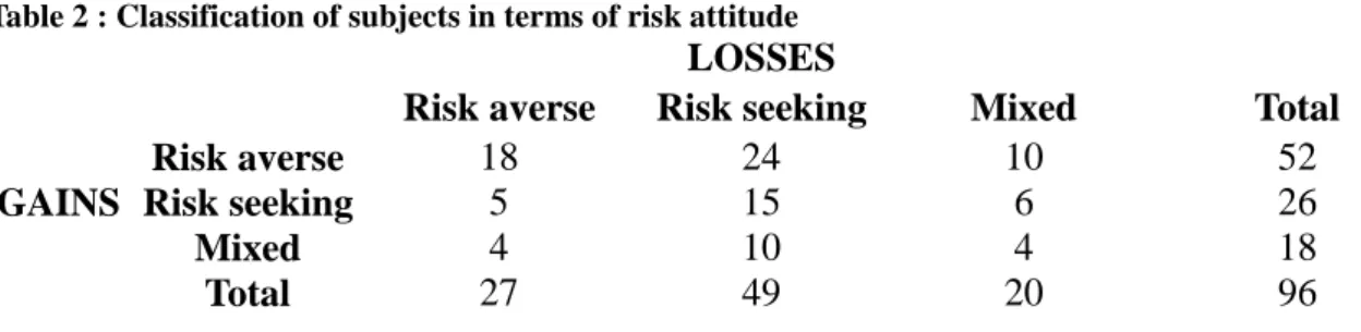
Table 2 : Classification of subjects in terms of risk attitude

LOSSES

Risk averse Risk seeking Mixed Total

Risk averse 18 24 10 52

GAINS Risk seeking 5 15 6 26

Mixed 4 10 4 18

Total 27 49 20 96

Following Abdellaoui et al. (2008), we classified a subject as risk averse (seeking) within each domain, if she was risk averse (seeking) for at least 4 out of 6 prospects in said domain. If a subject had exactly three risk averse and three risk seeking answers in one domain, then she was classified in the mixed category. As can be seen from table 2, most of our 96 experimental subjects cannot be classified as universally risk averse or risk seeking. Indeed, only 18 out of 96 subjects (19%) conform to the traditional assumption of global risk aversion. The majority pattern is one of risk aversion for gains (54%) and risk seeking for losses (51%), and the combination of the two is also the modal pattern at the individual level. The average loss aversion coefficient was 1.94.

More interesting in the present context are however representations at the individual level. Figure 6 shows some typical non-parametric probability weighting functions at the individual level for gains, assuming linear utility (typical functions for losses are similar). Subject number 50 can be seen to have (approximately) linear probability weighting. Subject 85 is optimistic, overweighting probabilities throughout, whereas subject 62 is pessimistic, underweighting probabilities

throughout. Subject 10 on the other hand displays the typical inverse-S pattern that is found to be prevalent at the aggregate level: overweighting of small probabilities, probabilistic insensitivity for the medium range, and hence underweighting of medium to large probabilities. For a more thorough discussion of such attitudes at the individual level and how to classify them, see Abdellaoui et al. (2011).

Fig. 6: typical probability weighting functions at the individual level, non-parametric 0 0.1 0.2 0.3 0.4 0.5 0.6 0.7 0.8 0.9 1 0 0.1 0.2 0.3 0.4 0.5 0.6 0.7 0.8 0.9 1 Subject n°10 Subject n°50 Subject n°62 Subject n°85

p w+(p)

Insensitivity

(overweighting of small probabilities and underweighting of medium to large probabilities)

Optimism (overweighting) Linear weights (expected utility) Pessimism (underweighting)

References

Abdellaoui, Mohammed (2000). Parameter-Free Elicitation of Utility and Probability Weighting Functions. Management Science 46(1), 1497-1512.

Abdellaoui, Mohammed, Aurélien Baillon, Laetitia Placido, and Peter P. Wakker (2011). The Rich Domain of Uncertainty: Source Functions and Their Experimental Implementation. American Economic Review 101, 695–723.

Abdellaoui, Mohammed, Han Bleichrodt, and Hilda Kammoun (2013). Do financial professionals behave according to prospect theory? An experimental study. Theory and Decision 74, 411-429.

Abdellaoui, Mohammed, Han Bleichrodt, and Olivier L'Haridon (2008). A Tractable Method to Measure Utility and Loss Aversion under Prospect Theory. Journal of Risk and Uncertainty 36, 245-266.

Agrawal, Anup, and Gershon N. Mandelker (1987). Managerial Incentives and Corporate Investment and Financiang Decisions. Journal of Finance 42(4), 823-837.

Baucells, Manel, Martin Weber, and Frank Welfens (2011). Reference Point Formation and Updating. Management Science 57(3), 506–519.

Bebchuk, Lucian A., Alma Cohen, and Holger Spamann (2009). The Wages of Failure: Executive Compensation at Bear Stearns and Lehman 2000–2008. Discussion Paper No. 657, Harvard Law School.

Bebchuk, Lucian Arye, and Jesse M. Fried (2003). Executive Compensation as an Agency Problem. Journal of Economic Perspectives 17(3), 71-92.

Benartzi, Shlomo, and Richard H. Thaler (1995). Myopic Loss Aversion and the Equity Premium Puzzle. Quarterly Journal of Economics 110(1), 75-92.

Bleichrodt, Han, Ulrich Schmidt, and Horst Zank (2009). Loss Aversion in Multiattribute Utility Theory. Management Science 55, 863-873.

Booij, Adam, Bernard M. S. van Praag, and Gijs van de Kuilen (2010). A parametric analysis of prospect theory’s functionals for the general population. Theory and Decision 68(1-2), 115– 148.

Carpenter, Jennifer N. (2000). Does option compensation increase managerial risk appetite? Journal of Finance 55, 2311–2331.

Charness, Gary, and Uri Gneezy (2012). Strong Evidence for Gender Differences in Risk Taking. Journal of Economic Behavior and Organization 83(1), 50–58.

Charness, Gary, and Matthew O. Jackson (2009). The Role of Responsibility in Strategic Risk Taking. Journal of Economic Behavior and Organization 69, 241–247.

Incentives: A Survey. Economic Policy Review, 27-50

Chou, Pin-Huang, Robin K. Chou, and Kuan-Cheng Ko (2009). Prospect theory and the risk-return paradox: some recent evidence. Review of Quantitative Finance and Accounting 33(3), 193– 208.

DeFusco, Richard A., Robert R. Johnson, and Tomas S. Zorn (1990). The Effect of Executive Stock Option Plans on Stockholders and Bondholders. Journal of Finance 45(2), 617-627.

Diecidue, Enrico, and Jeroen van de Ven (2008). Aspiration Level, Probability of Success and Failure, and Expected Utility. International Economic Review 49(2), 683–700.

Fellner, Gerlinde, and Matthias Sutter (2009). Causes, Consequences, and Cures of Myopic Loss Aversion – An Experimental Investigation. The Economic Journal 119(537), 900-916. Feltham, Gerald A., and Martin G.H. Wu (2001). Incentive Efficiency of Stock versus Options.

Review of Accounting Studies 6, 7-28.

Fiegenbaum, Avi (1990). Prospect Theory and the Risk-Return Association. Journal of Economic Behavior and Organization 14, 187–203.

Fox, Craig R., Brett A. Rogers, and Amos Tversky (1996). Options Traders Exhibit Subadditive Decision Weights. Journal of Risk and Uncertainty 13, 5-17.

Gneezy, Uri, and Jan Potters (1997). An experiment on risk taking and evaluation periods. Quarterly Journal of Economics 112, 631–646.

Greiner, Ben (2004). The Online Recruitment System ORSEE 2.0 - A Guide for the Organization of Experiments in Economics. University of Cologne, Working Paper Series in Economics 10. Guay, Wayne R. (1999). The Sensitivity of CEO Wealth to Equity Risk: An Analysis of the

Magnitude and Determinants. Journal of Financial Economics 53, 43–71.

Haigh, Michael S., and John A. List (2005). Do Professional Traders Exhibit Myopic Loss Aversion? Experimental Analysis. Journal of Finance 60(1).

Hall, Brian J., and Jeffrey B. Liebman (1998). Are CEOs really paid like beaurocrats? Quarterly Journal of Economics 113(3), 653–691.

Heath, Chip, Steven Huddart, and Mark Lang (1999). Psychological Factors and Stock Option exercise. Quarterly Journal of Economics 114(2), 601–627.

Holden, Richard T. (2005). The Original Management Incentive Schemes. Journal of Economic Perspectives 19(4), 135-144.

Holström, Bengt (1999). Managerial Incentive Problems: A Dynamic Perspective. Review of Economic Studies 66(1), 169–182.

Jegers, Marc (1991). Prospect Theory and the Risk-Return Relation: Some Belgian Evidence. The Academy of Management Journal 34(1), 215–225.

Jensen, Michael C., and Kevin J. Murphy (1990). CEO Incentives: It's Not How Much You Pay, But How. Harvard Business Review 3, 138-153.

Kahneman, Daniel, and Amos Tversky (1979). Prospect Theory: An Analysis of Decision under Risk. Econometrica 47(2), 263-291.

Köbberling, Veronika, and Peter P. Wakker (2005). An Index of Loss Aversion. Journal of Economic Theory 122, 119-131.

Lefebvre, Mathieu and Ferdinand M. Vieider (2013). Reining in Excessive Risk Taking by Executives: The Case of Accountability. Journal of Economic Behavior and Organisation, forthcoming.

List, John A., and Charles F. Mason (2010). Are CEOs expected utility maximizers? Journal of Econometrics, forthcoming.

March, James G. (1988). Variable Risk Preferences and Adaptive Aspirations. Journal of Economic Behavior and Organization 9, 5–24.

Mezias, Stephen J. (1988). Aspiration Level Effects: An Empirical Investigation. Journal of Economic Behavior and Organization 10, 389–400.

Pahlke, Julius, Sebastian Strasser, and Ferdinand M. Vieider (2011). Responsibility Effects in Decision Making under Risk. Working Paper.

Piron, Robert, and L. Ray Smith (1995). Testing risklove in an experimental racetrack. Journal of Economic Behavior and Organization 27, 465–474.

Schmidt, Ulrich, and Horst Zank (2008). Risk Aversion in Cumulative Prospect Theory. Management Science 54(1), 208-216.

Segal, Uzi, and Avia Spivak (1990). First Order versus Second Order Risk Aversion. Journal of Economic Theory 51, 111-125.

Smith C.W., and René M. Stulz (1985). The Determinants of Firms’ Hedging Policies. The Journal of Financial and Quantitative Analysis 20(4), 391-405.

Sutter, M., Huber, J., Kirchler, M. (2011). Bubbles and information: An experiment. Management Science (forthcoming).

Tversky, Amos, and Daniel Kahneman (1992). Advances in Prospect Theory: Cumulative Representation of Uncertainty. Journal of Risk and Uncertainty 5, 297-323.

Wakker, Peter P. (2010). Prospect Theory for Risk and Ambiguity. Cambridge University Press, Cambridge.

Weber, Martin, and Colin F. Camerer (1998). The Disposition Effect in Securities Trading: an Experimental Analysis. Journal of Economic Behavior and Organization 33, 167-184. Wiseman, Robert M., and Luis R. Gomez-Mejia (1998). A Behavioral Agency Model of

Managerial Risk Taking. Academy of Management Review 23(1), 133–153.

Wu, George, and Richard Gonzalez (1996). Curvature of the Probability Weighting Function. Management Science 42(12), 1676-1690.

Zeiliger, R. (2000). A Presentation of Regate, Internet Based Software for Experimental Economics, http://www.gate.cnrs.fr/~zeiliger/regate/RegateIntro.ppt, GATE. Lyon: GATE.