Adaptive sky detection and preservation in dehazing algorithm

Adaptive Sky Detection and Preservation in

Dehazing Algorithm

Sheng-kui Dai

College of Information Science and Engineering Huaqiao University Xiamen, China [email protected] Jean-Philippe Tarel LEPSiS, Cosys IFSTTAR Champs-sur-Marne, France [email protected]

Abstract—Single image defogging and/or dehazing algorithms usually emphasize the small intensity variations of the sky, when it is heterogeneous. This leads to a dramatic aspect of the restored image. This sky problem is probably one of the biggest defects of all the state-of-the-art dehazing algorithms. It was proposed to handle the sky problem by hard or smooth threshold of the sky area and to process the detected sky area differently not to emphasize too much the contrast of the sky heterogeneity. But the threshold value needed to be set by the user. We thus here propose a rule for selecting the threshold value as a function of the histogram of the image to process. This rule shows nice improvements on different kinds of images as shown in our experiments on a database of 1500 images.

Keywords—sky contrast preservation; defogging; dehazing; contrast restoration; histogram

I. INTRODUCTION

Due to the fog or haze, the contrast of a foggy image can be seriously decreased, as well as the color vividness. This may reduce the overall performance of real image or real video systems used in video surveillance, photography, intelligent vehicles...

Due to these many fields of application, defogging or dehazing has been a subject of interest in the recent years in image processing and computer vision. In the early works [1], [2], [3], [4], defogging required multiple images from the same point of view or, at least, an approximate 3D model of the scene. Recently, fog removal in the context of stereo reconstruction was also a subject of interest see [5] and [6]. However, the mainstream in fog removal remains single image defogging, where only the foggy image to be restored is assumed available. This is the case which corresponds to the larger field of practical applications.

The single image defogging algorithms proposed in the recent years can be grouped in three classes.

The first class consists in the use or in the improvement of standard algorithms for contrast enhancement, such as CLAHE [18], Retinex [17] or other algorithms developed originally, most of the time, for uniformly attenuated images. In these algorithms the fog physical model is not used and results are not correct in case of large depth variations in the observed scene.

The second class is based on a physical model of the fog, which is called Koschmieder’s law [9]. It is also the class of contrast restoration algorithms. For instance, Tan [7] removes fog by maximizing the local contrast of the result. But the enhanced sky is usually over contrasted. He et al. [10] proposed the Dark Channel Prior (DCP) but the sky area does not meet this prior and thus leads to bothersome color or contrast distortions. Tarel et al. [19] proposed fast defogging using median filter but they also face the sky problem. Kim et al. [8] can achieve nice results for most images, but sometimes there is a color cast in sky area. Very recently, Sulami et al. [11] obtained more vivid results but there are failure cases again in the sky.

The third class of algorithms uses a mixture of physically based and not-physically based processing. For instance, in [21] or [12], CLAHE is combined with contrast restoration such as DCP.

Despite the fact that the sky area is usually over contrasted in single image defogging, we only found two articles [13] and [14] on how to fix the sky problem for images under daylight. The success of these two algorithms deeply relies on the choice of a parameter value used to detect the sky. This value is usually different from one image to another.

This paper is organized as follows. Section 2 recalls the general approach of the single image contrast restoration. Section 3 describes the proposed rule to detect the sky in the image and to select the sky threshold. Section 4 reports the experimental results obtained with the proposed algorithm and a user evaluation.

II. CONTRAST RESTORATION APPROACH A. Fog model

Koschmieder’s law has been established as a simple model of the atmospheric effects of fog or haze on the observed image I(x), see [9]: )) x ( t 1 ( ) x ( t ) ( ) x ( =J x +A − I (1)

where x stands for the pixel coordinates, J(x) is the haze-free image we would like to obtain, A is the sky light, and t(x) in [0,1] is the transmission rate indicating the portion of the light that is not scattered and reaches the camera. The transmission rate is an exponential attenuation function of the distance between the object and the camera. In single image defogging, the image I(x) is known and we are seeking for J(x) from (1).

B. Transmission Inference

The single image defogging problem being ill-posed, extra assumptions are needed to infer a reasonable transmission map. Several assumptions were proposed in the past, such as DCP [10] or NBPC [20]. The use of one or another of these assumptions usually leads to infer the atmospheric veil, which is the complementary of the transmittance map, as a low-pass filtering of the observed image. Examples of such filtering are:

- Gaussian or mean filtering on the gray level image, - minimum over the color channels followed by an erosion or a dilation filter, also named DCP [10],

- minimum over the color channels followed by a median filter, like in [19],

- minimum over the color channels followed by a bilateral filtering, like in [13],

- interpolation obtained during CLAHE algorithm as proposed in [21].

However, after this filtering step, the obtained transmittance map is not perfect, because the assumption is never perfectly verified on the whole image or for all objects geometrical configurations. It follows that one more step is necessary most of the time in order to refine the transmittance map. As pointed in [20], this step can be performed by any filter able to smooth the previously obtained transmittance map at all pixels where no edge is detected in the observed image I(x). For the refinement step, different filters where proposed such as: soft matting [10], guided filter [15], joint/cross bilateral filter [20], guided bilateral filter [22].

C. Contrast Restoration

The sky light A can be estimated by various techniques such as the one proposed in [10]. The transmission t(x) and A being inferred, the restored image can be deduced by inversing (1) as: A A I J = − + ) t ), x ( t max( ) x ( ) x ( 0 (2)

where a threshold t0 is applied on the transmission to prevent division by very small values. The usual value for t0 is 0.1.

D. Sky area Preservation

Two variants of the DCP algorithm are able to preserve the sky area. The first one, the so-called Improved Dark Channel Prior (IDCP), uses a hard threshold [13], while the second one uses a soft threshold [14].

D1. Improved Dark Channel Prior

(a) (b) (c) (d)

(e) (f) (g) (h)

Fig. 1: Sky area obtained for different algorithms for two images. (a), (e) foggy images; (b), (f) results with DCP; (c), (g) results with the sky area preservation proposed in [13] using K=50; (d), (h) results with the sky area preservation

proposed in [14].

The IDCP [13] consists in two variations. First, the value p within [0.08,0.25] is added to the transmittance:

p x t x

t1( )= ( )+ (3) This increase of the transmission rate leads to a clearer restoration result which is beneficial to the sky region. Second, the sky area is segmented from the foggy image using a threshold of value K and the transmission is set to 1 in the sky area: ⎩ ⎨ ⎧ > − ≤ − = K | A (x) if (x) t K | A (x) if 1 (x) t 1 2 |I |I ₍₄₎

The value of K proposed in [13] is 50, but as shown in Fig. 1(c) and Fig. 1(g) it is not always the same value which must be used. The value of K is a function of the image. Moreover, the use of a hard threshold introduces an intensity discontinuity in the result images.

D2. Tolerance mechanism

In [14], it is proposed to modify the t(x) obtained from DCP using the following equation:

⎟⎟ ⎠ ⎞ ⎜⎜ ⎝ ⎛ × ⎟⎟ ⎠ ⎞ ⎜⎜ ⎝ ⎛ − = ,1 max(( ), ),1 | ) ( | max min ) ( 0 1 t x t A x I K x t (5)

where K is again the threshold value on the sky intensity, with 50 as the default value, as explained in [14]. As shown in Fig. 1(d) and Fig. 1(h), obtained results are more continuous compared to IDCP, thanks to the use of the soft threshold. Nevertheless, the main limitation of [14] is that the intensity parameter K must be set by the user depending on the image content. For example, the default value K=50 is suitable in Fig. 1(d), but it is not appropriate in Fig. 1(h). Indeed, it can be observed that the upper area of Fig. 1(h) is less defogged, which makes the objects in this area not as clear as those in Fig. 1(f). In addition, the sky and road regions are a little darker than those in Fig. 1(c) and Fig. 1(g). This shows the necessity to have a way to estimate the value of K as a function of the image content.

III. PROPOSE THRESHOLD ESTIMATION

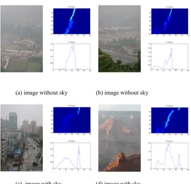
We seek to relate the value of the parameter K to the content of the image and more precisely to the intensity histogram of the image. In a first analysis, we used the four images shown in Fig. 2. The first two images, shown in Fig. 2(a) and (b), were selected for the difficulty to distinguish the sky region from the ground objects. The two images shown in Fig. 2(c) and (d) were selected for the distinct sky area and for gray ground objects. By experimental testing, we found the good values of parameter K are about 1, 3, 40 and 50 respectively for these 4 images. So the first observations are that the range of appropriate K values is quite large, and that the brighter the sky, the higher the value of K.

The histograms of the four images are also shown in Fig. 2. From these histograms, it seems possible to distinguish images with a distinct sky area from those without. Indeed, the images with a distinct sky area show a strong peak in the 1D histogram for large intensities. Therefore, it is reasonable to decide on the presence of a sky area in a given image based on the presence of a strong peak in its histogram

The algorithm to detect if the sky is seen in the image is in six steps, followed by one step for sky threshold estimation and a final step for restoration:

Step 1: Seek the upper bound Iub of the searching interval to:

⎭ ⎬ ⎫ ⎩ ⎨ ⎧ ≤ ≤ > =

∑

where hist() is the intensity histogram of the image. Due to noise and the presence of light sources in the image, the controlling parameter k1 can be set to 0.99.

Step 2: Seek the lower bound Ilb of the searching interval to:

⎭ ⎬ ⎫ ⎩ ⎨ ⎧ ≤ ≤ > =

∑

where the controlling parameter k2 should be greater than 0.50, and it is set simply to 0.50 in this paper.

(a) image without sky (b) image without sky

(c) image with sky (d) image with sky

Fig. 2: typical images (left) and their 2D (up) and 1D (down) intensity histograms..

Step 3: The intensities of the sky being bright in a day-light

image, they should be included in the previously defined search interval [Ilb, Iub]. The upper bound of the sky intensity interval is obviously set to Iub. To find the lower bound of the sky intensity interval, we seek the lowest valley in the search interval. The location Ivalley of this valley gives the lower bound of the sky intensity interval and is defined as:

{

}

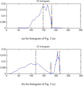
Rather than the Iub bound, the Iub-5 bound can be used to enforce a minimal distance between Ivalley and Iub. In Fig. 3, as an illustration, the three key intensities are shown in two different histograms. The position of Ilb in histogram is displayed with symbols ♦, Iub with symbols +, and Ivalley with symbols o.

Step 4: The sky intensity interval being defined, we now decide if the sky is visible or not in the image. When the sky is visible, we expect an important peak in the sky intensity interval. This peak must be higher than the lower bound of the histogram, and it must have a significant surface. The rule to decide if sky is visible or not is thus:

⎪ ⎪ ⎩ ⎪⎪ ⎨ ⎧ < > > − = eithers , 0 ) ( ) ( and and if , 1 ub 5 4 3 ub I hist k I hist k I k I I SkyFlag valley sum valley (9)

where Isum is the sum of hist() in the sky intensity interval

[Ivalley, Iub]. This rule requires to set a threshold value k3 for the

peak width, a threshold value k4 for the peak area and a

threshold value k5 for the difference between the intensity at

Ivalley and the intensity at Iub. Based on experiments on our

image-database, empirical value are k3=10, k4=0.04 and k5=2.

(a) for histogram of Fig. 2 (a)

(b) for histogram of Fig. 2 (c) Fig. 3: key intensities on image histograms.

Step 5: When SkyFlag is 0 (false), the sky is not found visible in the image so there is no need for sky preservation. Thus K is set to zero or one. When SkyFlag is 1 (true), we relate K with the width Iub−Ivalley of the sky intensity interval.

Indeed, K can be also defined as the size of the sky intensity peak. In practice, to achieve best results, K is computed as a factor of Iub-Ivalley. This factor k6 uses a fixed value. As a consequence, the parameter K can be simply estimated as

K = SkyFlag*(Iub-Ivalley)*k6 +1 (10) where k6 is fixed to 1.5 in practice whereas it should be 1.0 in theory. In order to prevent too large values for K, it is clipped using the following saturation function:

K ’= 2*K/(1+K/k7) (11) where the empirical value of k7 is 30 in practice.

Step 6: The sky being detected and K being estimated, the defogging step can be performed. To estimate the transmission

t(x), rather than use equations (3) and (4) or (5) after

transmission estimation, a modified intensity image I’ is used as input for transmission estimation. This modified image is defined as a function of the original image and K’:

) ( 1 , ' | ) ( | min ) ( ' I x K A x I x I ⎟× ⎠ ⎞ ⎜ ⎝ ⎛ − = (12)

Equation (12) linearly modifies the intensities between A and A-K. When, the sky is detected in the input image, pixels with intensity lower than Ivalley will not be changed, but sky pixels are attenuated linearly down to 0 when I(x) equals A. This will reduce the estimated transmission for sky pixels, and preserve the sky after application of equation (2). Fig. 4 shows the function (12) on an intensity histogram.

Fig. 4: Linear attenuation (12) to handle the sky during transmission computation.

Notice that with the proposed approach, any kind of defogging algorithm can be combined with automatic sky detection and preservation.

IV. EXPERIMENTS

Our testing platform includes the software Matlab (2012a) running on a win64 system, and fast bilateral filter [16] is adopted for transmission evaluation.

In Fig. 5, a few comparative results with and without automatic sky area preservation are shown on the images of Fig. 2(c) and Fig. 2(d). Estimated parameters are K=38.4 and

K=36.3, respectively.

Fig. 5: Comparison for the images of Fig. 2 (c) and Fig. 2 (d). From left to right, the transmission map obtained without sky area preservation, restoration

result, the modified transmission map using the proposed method and the restoration result.

In order to evaluate the proposed method of automatic sky detection and sky area preservation, a database of 1500 foggy images was collected from the internet and from previously published articles on defogging (see Fig. 6 for samples).

Defogging with and without sky detection and sky area preservation was applied to all the images in the database. Seven students knowing image processing were asked to evaluate the presence of sky in the image and to compare between defogging with and without the proposed method. The results of the two methods were of course presented in a random order. Statistics on the experimental results show that the proposed sky detection method correctly classify 90% of the images of the database. Tab. 1 reports the evaluations of the seven observers. When the sky is not detected, the sky area

preservation is not applied. This is why most of the time, observers told that the two images are the same.

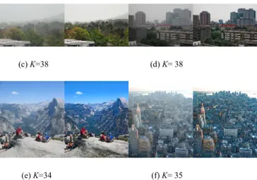
Fig. 6: part of the 1500 images in the evaluation database. For image with sky area, the proposed algorithm provides better results for 45% images, no difference for 42% images, less good for 8% pictures and 5% images are difficult to judge. In the Fig. 7, results for images with sky are shown with estimated K before and after defogging. In the Fig. 8, results for images without sky are shown before and after defogging (K=1). In Fig. 9 are shown a few results not satisfying us. In Fig. 10, a few images wrongly estimated without sky are shown with restoration. As shown in Tab. 1, there are relatively few such erroneous cases.

Tab.1 : classification results for several observers ( comparison of results with/without sky area preservation )

Image with sky Image without sky

better same worse other better same worse other

(1) 499 402 6 51 3 523 7 9 (2) 447 512 38 114 0 374 4 11 (3) 445 562 154 0 2 329 8 0 (4) 525 489 60 59 6 354 6 1 (5) 590 425 149 5 11 311 9 0 (6) 437 395 138 123 21 352 28 6 (7) 529 500 95 41 15 303 16 1 me an 496 469 91 56 8 363 11 4 (a) K=36 (b) K=35 (c) K=38 (d) K= 38 (e) K=34 (f) K= 35

Fig. 7: Result on first case. Left to right: typical foggy images with sky and the defogging results with their controlling parameter K (left: foggy image, right:

defogged image)

Fig. 8: Result on second case. Left to right: foggy image without sky and its defogged result, and since SkyFlag=0, we always have K = 1.

(a) No.0067, K=44

(b) No.0106, K=42

Fig. 9: Result on third case. Fog decision is right (SkyFlag=1) but the obtained result is not satisfying for these images. Left to right: original image, result

without/with sky area preservation.

(a) No.0094 , K=1

(b) No.0887, K=1

(c) No.1035 K=1

Fig. 10: Result on fourth case. Left to right: fog decision is wrong (SkyFlag=0). The peak in the histogram (in the middle) does not satisfy formula (9).

V. CONCLUSION

In this paper, we propose a method for automatic sky detection and sky area preservation during defogging. The sky detection consists in finding a strong peak in the right part of the intensity histogram. Sky area preservation consists in a smooth threshold where the threshold is estimated from the size of the sky peak. This algorithm can be applied to all defogging algorithms based on Koschmieder’s law for the fog model. Experimental results with a database of 1500 images show that the proposed improvement is effective.

Acknowledgment: this paper is jointly sponsored by China Scholarship Council (CSC) and Institut français des sciences et technologies des transports, de l'aménagement et des réseaux (IFSTTAR). All the authors would like to thank IFSTTAR to invite the first author as a visiting scholar to do this work together with Prof. Jean-Philippe Tarel at IFSTTAR.

REFERENCES

[1] F.Cozman and E.Krotkov, "Depth from scattering", IEEE Conference on Computer Vision and Pattern Recognition, vol. 31, pp. 801-806, 1997.

[2] S.G.Narasimhan and S.K.Nayar, "Chromatic Framework for Vision in Bad Weather", IEEE Conference on Computer Vision and Pattern Recognition, vol. 1, pp. 598-605, 2000.

[3] Y.Y.Schechner, S.G.Narasimhan, and S.K.Nayar, "Instant Dehazing of Images using Polarization", IEEE Conference on Computer Vision and Pattern Recognition, vol. I, pp. 325-332, 2001.

[4] S.G.Narasimhan and S.K.Nayar, "Contrast restoration of weather degraded images", IEEE Transactions on Pattern Analysis and Machine Intelligence, vol. 25, no. 6, pp. 713-724, 2003.

[5] L.Caraffa and J.-P.Tarel, "Stereo Reconstruction and Contrast Restoration in Daytime Fog", IEEE Asian Conference on Computer Vision, Part IV, pp. 13-25, Nov 2012.

[6] Y.Lee, K.B.Gibsony, Z.Lee, and T.Q.Nguyen, "Stereo Image Defogging", IEEE ICIP, pp. 5427-5431, 2014.

[7] R.T.Tan, "Visibility in bad weather from a single image", IEEE Conference on Computer Vision and Pattern Recognition, pp. 1-8, 2008. [8] J.H.Kim, W.D.Jang, J.Y.Sim, and C.S.Kim, "Optimized contrast

enhancement for real-time image and video dehazing", J. Vis. Commun. Image R. vol.24, pp. 410-425, 2013.

[9] W.Middleton, "Vision through the atmosphere", University of Toronto Press, 1952.

[10] K.He, J.Sun, and X.Tang, "Single image haze removal using dark channel prior", IEEE Conference on Computer Vision and Pattern Recognition, pp. 1957-1963, 2009.

[11] M.Sulami, I.Glatzer, R.Fattal, and M.Werman, "Automatic Recovery of the Atmospheric Light in Hazy Images", IEEE International Conference on Computational Photography, pp. 1-11, 2014

[12] T.Arora, G.Singh, "Evaluation of a new Integrated fog removal algorithm IDCP with CLAHE", Proceedings of IRF International Conference, pp. 46-52, 2014.

[13] H.R.Xu, J.M.Guo, Q.Liu, and L. L. Ye, "Fast Image Dehazing Using Improved Dark Channel Prior", IEEE International Conference on Information Science and Technology, pp. 663-667, 2012.

[14] Z.H.Liu,Y.X.Yang, and J.Y.Yang, "Single Aerial Image De-Hazing and Its Parallel Computing", Journal of Surveying and Mapping Engineering, Vol.1 Iss.2, pp. 33-40, 2013

[15] K.M.He, J.Sun, and X.O.Tang, "Guided Image Filtering", IEEE Transactions on Pattern Analysis and Machine Intelligence, vol.35 Issue No.06, pp. 1397-1409, 2013.

[16] J.Chen, S.Paris, F.Durand, "Real-time Edge-Aware Image Processing with the Bilateral Grid", SIGGRAPH ’07, Article No. 103, 2007. [17] D.Jobson, Z.Rahman, and G.Woodell, "A multiscale retinex for

bridging the gap between color images and the human observation of scenes", IEEE Transactions on Image Processing, vol. 6, no. 7, pp. 965– 976. 1997.

[18] K.Zuiderveld, "Contrast limited adaptive histogram Equalization", Graphics gems IV. San Diego, USA: Academic Press Professional, Inc., pp. 474–485. 1994.

[19] J.-P.Tarel, and N.Hautière, "Fast Visibility Restoration from a Single Color or Gray Level Image", IEEE International Conference on Computer Vision, Japan, pp. 2201–2208, 2009.

[20] J.-P.Tarel, N.Hautière, L.Caraffa, A. Cord, H. Halmaoui, and d. Gruyer, "Vision Enhancement in Homogeneous and Heterogeneous Fog", IEEE Intelligent Transportation Systems Magazine, Vol. 4, No. 2, pp. 6–2, 2012.

[21] H.Halmaoui, A.Cord, N.Hautière, "Contrast restoration of road images taken in foggy weather", 2011 IEEE Int. Conf. Computer Vision Workshops (ICCV), pp. 2057–2063, 2011.

[22] L.Caraffa, J.-P.Tarel and P.Charbonnier, "The Guided Bilateral Filter: When the Joint/Cross Bilateral Filter Becomes Robust", to appear in IEEE Transaction on Image Processing, 2015.