3D Node Deployment Strategies Prediction in Wireless Sensors Network

Any correspondence concerning this service should be sent

to the repository administrator:

tech-oatao@listes-diff.inp-toulouse.fr

This is an author’s version published in:

http://oatao.univ-toulouse.fr/25045

To cite this version:

Nasri, Nejah and Mnasri, Sami and Val,

Thierry 3D Node Deployment Strategies Prediction in Wireless

Sensors Network. (2019) International Journal of Electronics, 1. 1-30.

ISSN 0020-7217

Official URL

DOI :

https://doi.org/10.1080/00207217.2019.1687759

Open Archive Toulouse Archive Ouverte

OATAO is an open access repository that collects the work of Toulouse

researchers and makes it freely available over the web where possible

1

Abstract— 3D Deployment represents a fundamental role in setting up an efficient wireless sensor network (WSNs) and IoT network. In general, WSN are widely used in a variety of applications ranging from monitoring a smart house to monitoring forest fires with parachuted sensors. In this paper, we focus on planned 3D deployment, which the sensor nodes must be accurately positioned at predetermined locations to optimize one or more design objectives under some given constraints. The purpose of planned deployment is to determine the type, number, and locations of nodes to optimize coverage, connectivity and network lifetime. There have been a large number of studies, which proposed algorithms for solving the premeditated 3D deployment problem. The objective of this paper is twofold. The first one is to present the complexity of 3D deployment and then detail the types of sensors, objectives, applications and recent research that concerns the strategy used to solve this problem. The second one is to present a comparative survey between recent optimization approaches used to resolve the deployment problem in WSN. Based on our extensive review, we discuss the strengths and limitations of each proposed solutions and compare them in terms of the WSN design factors.

Index Terms _{Indoor Environments, Optimization, Coverage,}

Connectivity, Energy consumption, Wireless Sensor Networks.

I. INTRODUCTION

A fundamental problem in the WSN and IOT collection network is how to deploy the sensors. The deployment problem can be described as follows: Having N wireless sensors and an area A to cover. How to deploy these sensors to form a WSN that meets system requirements, such as the connectivity of the network, its ability to detect relevant events happening in A, and is the ability to provide a required period of operation. This problem is related to coverage, connectivity, and lifetime issues. Indeed, the problem of deployment in WSN refers to the determination of the positions of nodes (and/or the base stations) so that the coverage, the connectivity and the energy efficiency can be obtained with a minimum number of nodes.

Events happening in an area lacking a sufficient number of nodes may be unnoticed. Moreover, areas with dense sensor populations suffer from congestion, redundancy detection, and delays. Optimal deployment ensures adequate quality of

service, long network life and cost saving. The problem of deployment can also be defined as follows: having a surface A in 2D or 3D with a set of obstacles (that can exist without partitioning A), and a set of sensors having different types (according to the radii of detection and communication). The overall goal is to minimize the number of nodes to be deployed on A while ensuring one or more objectives such as network coverage and connectivity [1]. It is said that the target region is covered if each point in A is covered by an active sensor having a probability of coverage Pc and a sensing range Rs if there is direct communication (Line of Sight) without or in the presence of obstacles. Besides, it is said that the network monitoring a target region is fully connected if all sensors can route data in multi-hop to the base station or another destination node.

Most deployment approaches consider a WSN with randomly deployed sensors, which are generally modeled by a Poisson point process with a density γ. This Poisson process is defined as follows: for any zone A in the region R, the distribution of the number of nodes in A is the mean distribution of Poisson γǁAǁ, ǁAǁ is the surface of A. Given the number of nodes, their locations are mutually independent random variables and uniformly distributed over A. It is known that n nodes whose locations are mutually independent random variables, with a uniform distribution within A, are mainly a Poisson process with a density γ, provided that A is large [2].

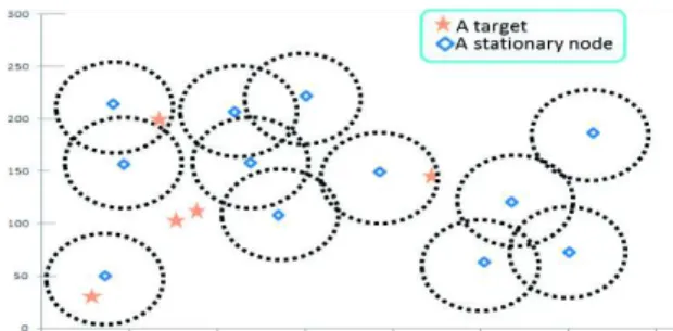
An example of randomly deployed sensor networks is shown in Figure 1. There are twelve sensors deployed in a rectangular detection field. The density of sensors on the left side of the field is higher than that on the right one. Therefore, the detection field is not fully covered by the sensors.

Figure 1. An example of area coverage using randomly deployed sensors

3D Node Deployment Strategies Prediction in

Wireless Sensors Network

Nejah NASRI

, Sami MNASRI

, Thierry VAL

Department of Electrical Engineering, School of Sfax, University of Sfax, Sfax, Tunisia

(nejah.nasri@isecs.rnu.tn)

2

University of Toulouse, UT2J, CNRS-IRIT-IRT, Toulouse, France

(

val@irit.fr

)

3

Faculty of Sciences of Gafsa,UPIM (Physics, Informatics and Mathematics Unit), Gafsa, Tunisia

(

Sami.Mnasri@fsgf.rnu.tn

)

Finding the optimal node distribution is a difficult problem to solve and it is considered NP-hard for most formulations. This problem is proven to be optimally solved in 2D environments while it has been proven NP-difficult if it is generalized to 3D environments [3]. Figure 2 shows an example of 2D deployment and another for 3D deployment.

2D deployment 3D deployment

Figure 2. 2D deployment vs. 3Ddeployment

When sensors are deployed randomly, the initial coverage area provided by the network cannot be optimal as in the case of deterministic deployment. In order to increase the covered area, redundant sensors are deployed. Redundancy makes sensor networks denser than normal ad hoc networks. However, increasing sensor density cannot provide a 100% coverage probability. Even more, it is expensive to maintain high-density WSN on a large scale. Therefore, other approaches should be used to avoid these problems and improve the coverage after the initial random deployment. Another problem that complicates the redeployment is that of the robustness of WSN. Indeed, once deployed, it is expensive and impractical, even impossible, to replace unusable sensors in most types of applications. Hence, if a particular node is no longer running, there will be an impact on the overall performance of the network. The loss of a node may be due to different causes, such as battery depletion, physical damage caused by environmental forces, or destruction by the enemy. If a sensor that covers a sensitive area dies and no other sensor can cover that area, the WSN fails its mission of efficiently distributing the sensors.

Indeed, one way to optimize the distribution strategy in WSN is to have redundant sensors that improve the performance of the network. In addition, if the detection field is vast or has limited access, the sensors may not be able to be deployed one by one in specific locations. Instead, they can be disseminated from an airplane. When the sensors are randomly deployed, the initial coverage area provided by the network cannot be optimal as in the case of deterministic deployment. In order to increase the coverage area, redundant sensors can be deployed. Redundancy makes sensor networks denser than ad hoc networks.

However, increasing sensor density cannot provide a 100% coverage probability. Even more, it is expensive to maintain high-density sensor arrays on a large scale. Therefore, other approaches should be used in order to avoid these problems and improve the coverage after the initial random deployment. Another problem that complicates the redeployment is the robustness of WSN [4]. Once deployed, it is expensive and impractical, if not impossible, to replace unusable sensors in

most types of applications. Therefore, if a particular node is no longer running, there will be an impact on the overall performance of the network.

The process of deploying the sensor nodes greatly influences the performance of a WSN. The problem of deployment or positioning nodes in a WSN is a strategy that defines the topology of the network, and therefore the number and position of nodes. The quality of monitoring, connectivity, and power consumption are also directly affected by the network topology.

The different deployment tasks can be grouped into three main phases. A pre-deployment and deployment phase (Figure 3 (a)) which is achieved by the manual placement of nodes or the spreading of nodes from a helicopter, for example. A phase of post-deployment (figure 3 (b)) is necessary if the topology of the network has evolved, for example following a displacement of nodes, or a change of the radio propagation conditions. The third phase concerns the redeployment (Figure 3 (c)) which is based on adding new nodes to the network in order to replace some failed nodes. The system can iterate on phases 2 and 3.

(a) Pre-deployment and deployment phase

(b) Post-deployment phase

(c) Redeployment phase Figure 3. Phases of deployment [22]

Different issues are encountered at the level of the deployment of sensor nodes in WSN. These studies mainly concern stationary and mobile cases, single and multi-objective cases, deterministic and stochastic aspects, and finally static and dynamic deployments [5].

Authors in [6] and [7] proposed a detailed study of deployment in the static case. They distinguish two deployment methodologies according to the distribution of the nodes (either random or controlled). The treated primary objectives can be as follows:

- The coverage, which is one of the most preponderant problems in WSN. Several types of coverage are presented: point coverage, area coverage, barrier coverage and coverage of an event or a moving target.

- The consumed energy and ensuring the energy efficiency. - The network connectivity.

- The lifetime of the network. - The network traffic. - The reliability of data.

- The cost of deployment (depending on in terms of a number of deployed nodes).

- The fault tolerance and load balancing between nodes. In the context of dynamic deployment, authors in [8]

investigate the research works proposing solutions for the sensor nodes repositioning and its related issues. Connectivity and coverage are the most used factors in determining the communication and the detection efficiency, respectively. The coverage is affected by the sensitivity of the sensors represented by the detection range (noted Rs), while the connectivity is guaranteed by the communication range (noted Rc). According to [8], the degradation of the coverage probability in some WSN applications is tolerable, whereas the degradation of the probability of connectivity could be fatal for the network.

Technological advances on the construction and manufacture of sensors have made them smaller, more affordable and more reliable. This allowed broadening the range of targeted application areas. The integration of WSN technology in industry has improved the business performance. Still more experimental work is needed to increase the reliability and efficiency of real-world WSN use. Given the variety of sensors, the applications of deployment sensors are very varied.

In ecological applications, WSNs deployments are used to optimize the use and consumption of energy resources, such as a sensor incorporated into an air-conditioning system in a building. Indeed, this network manages the air conditioning according to the location of the individuals. The air conditioning trips only if it is necessary. For example, when the sensor detects the existence of people in the Region of Interest (RoI). This is the case for a heating, lighting or ventilation systems. In traceability and localization applications, WSN deployment can be a major fault correction of Global Positioning System (GPS) systems, which are high-energy consumption. Indeed, people who ski can be equipped with sensors. These sensors will be handy to locate victims under snow in case of an avalanche. Several other traceability and localization applications with significant economic interests can be considered. Again, unlike location solutions that are based on GPS systems, WSNs allow their deployment in enclosed areas such as mines or underwater areas [9].

In industrial applications, the deployment reduces the cost of maintenance constraints. Optimal sensors deployment can enhance manufacturing activities and it is ideal for any activity that requires fixed location and limited resources. Several other constraints and restrictions can be solved using WSNs. Among others, weight restrictions (in an airplane for example) and mobility ones (tracking a moving target or detecting a robot movement). Among industrial WSN applications, we can mention the following ones: Surveillance and monitoring activities on hazardous conditions (radioactivity exposure, etc.); Monitoring polluted geographical areas or real-time monitoring of a contaminated area to draw a dynamic

geographical map; Monitoring the operation of machines; Logistics and inventory control; Process monitoring and traffic monitoring; Preventive maintenance of equipment and structures and supervision of foundations and buildings in civil engineering.

In security applications, deployment can limit the financial expenses of securing structures. Among the WSN security applications: The deployment of sensors for detecting cracks and alterations in structures and buildings, following an earthquake or just to control its aging. This deployment can anticipate the destruction of the structure. Monitoring of movements in a geographical area to set up a distributed system of intrusion detection. The distributed aspect of different systems makes it possible to cross it or put it in a state of dysfunction.

In environmental Applications: To ensure broad coverage over a large geographic area, an optimal WSN deployment can be used. We can cite several typical WSN environmental applications: Dissemination of a temperature-sensitive sensors on a forest (deployment from an airplane) to detect the outbreak of a fire; Controlling and managing the irrigation of green surfaces by detecting dry areas; The deployment of sensors on industrial sites, nuclear structures or oil refineries to capture and report the existence of leaks of toxic products (gases, chemicals, etc.) for rapid and effective intervention and the control of natural parks, sensors can be deployed to monitor animal movements and activities or to report and provide information on seasonal migrations of birds.

In medical and veterinary applications: WSN deployments are generally used to permanently monitor patients. They are deployed to collect physiological data on vital functions such as heart rate, glucose levels, respiration or blood pressure. This facilitates the real time diagnosis of diseases and the monitoring of patients' health status. These sensors can be implanted under the skin or worn by the patient.

In the military field, WSNs are often deployed to monitor or analyze strategic areas, providing information regarding the loss or damage after a battle, monitoring the enemy equipment and ammunition, detecting chemical or nuclear attacks, etc.

In smart homes and commercial applications: WSN can also be used in a commercial context. Indeed, sensors can control the operations of storage and delivery and provide (in real time) information about conditions, directions or positions of the goods. We can also follow production chains in factories and control the entire production process. Another very practical commercial WSN use is that of smart homes (Figure 4). Figure 5 illustrates the intelligent home of the IUT of Blagnac in Toulouse in which our experiments are carried out. This application mostly targets people with disabilities or elderly to ensure their safety. Among the services offered in this context, the automatic control of doors and curtains (closing and opening), the control of household appliances (activation or shutdown), the triggering of the watering of plants in the garden or the management of air-conditioning and heating systems.

Figure 4. Illustration of a smart home

Figure 5. Our smart home (Blagnac, Toulouse)

Table 1 illustrates different recent deployment applications: TABLE I. RECENT DEPLOYMENT APPLICATIONS

Paper Application(s)

Boubrima et al. [10] Mobile WSN,air surveillance

applications Shehu et al.[11]

Signal detection

Segmentation of grayscale images by multi-level thresholding Han et al.[12] disaster management, localization Mostafaei et al.[ 13] Border surveillance

Gjanci et al.[14] Acoustics WSN; submarines WSN Adame et al.[ 15] Surveillance of the elderly persons and

smart homes Kumar et al.[ 16] Precision agriculture

The originality of this study is that it relies on different angles of views: a global analysis of the deployment problem is suggested by discussing the common models and assumptions, then detailing the approaches adopted in the literature. Indeed, the main contributions of this survey can be

summarized as follows:

-This survey gives a comparative study with a sophisticated classification, which relies on the type of modeling, and gives the recent art state of the deployment resolution approaches. -Comprehensive definitions of connectivity and coverage with their different variants are given. For a better understanding, the connectivity and coverage problems are defined together then separately in this survey.

-Current trends and open issues of the deployment are discussed and summarized.

-Using the 3D deployment problem as an example, this study proves the efficiency of the optimization algorithms in solving complex real world problems.

The rest of the paper is organized as follows. In Section II,

we present an overview of 3D WSNs deployment. Specifically

we define deployment strategies, types of deployment and different sensing model for WSNs. Section III, explores 3D multi-objective deployment, particularly we define primary objectives for 3D deployment. In section IV, we present a

comparison and a review of recent studies over WSNs deployment. Section V illustrates numerical results of the recent approaches resolving the WSN deployment. Section VI gives a discussion of trends and present open deployment issues. Finally, section VII gives a conclusion and a set of perspectives.

II. OVERVIEW OF 3D DEPLOYMENT IN WSN

When designing deployment strategies, several factors must be considered such as the monitoring area, the sensor capabilities (detection range and transmission range), the zone coverage, and the lifetime of sensors. The following questions should also be considered when establishing a deployment strategy: How many sensors should be deployed? How to place sensors in the monitoring area? Where to put the base station (BS) if we can choose its position? The number of sensors can be deduced from the lower limit of the monitoring area, sensor capacity and design requirements.

II.1 CLASSIFICATION OF COVERAGE There are three types of coverage issues:

II.1.1 Full coverage

Full coverage is achieved if every point in the 3D RoI is at least covered by a sensor. Full area coverage requires the deployment of a large number of sensors, which increases cost and complexity. However, partial coverage only guarantees a certain percentage of coverage [17]. Figure 6 illustrates different geometric layouts used in the 3D coverage.

Figure 6. Different geometric 3D coverage layouts [18]

II.1.2 K-coverage

With regard to the coverage, 3D RoI is assumed to be k-covered if there are at least k sensors that cover and monitor each point of the 3D RoI [18]. Indeed, k-coverage represents the logical extension of the case of 1-coverage. In the case of k-coverage, the distance between the detection nodes is minimized with the appearance of overlaps between the detection spheres. In general, when achieving the k-coverage optimally (K>1), the complexity of the coverage algorithm will increase.

II.1.3 Surface coverage

In the case of surface coverage (shown in Figure 7), the sensors can only be deployed on the surface of the RoI. Many real applications require this kind of surface coverage where the RoI is a complex surface that is not a complete 3D space or a 2D plane. Mathematically, the detection field can be modeled as several small simplified triangles as single-valued function z = f (x,y) with two node distribution models: a planar surface Poisson point model and a space surface

Poisson point one [2]. In [19] authors address the problem of surface coverage of 3D terrains in Mobile Wireless Sensor Networks.

Figure 7. 3D surface coverage [1]

II.2 TYPES OF DEPLOYMENT

Deployment in WSN can be classified based on the placement strategy, applications and deployment domain. However, existing schema of deployment can be categorized under multiple criteria.

II.2.1 Single Objective Deployment vs. Multi-Objective Deployment

The criteria and objectives, on which the deployment is optimized, are often contradictory. This is the case of coverage and energy consumption or survivability and fault tolerance. Therefore, we cannot find a deployment that optimizes all objectives simultaneously. Hence the need for an optimal trade-off between the different objectives. According to the used type of deployment (single or multi-objective), we can either optimize each objective alone or use an aggregation function that combines all objectives in a single function with weights that represent the importance of each objective.

II.2.2 Deterministic deployment vs. stochastic deployment

The selection of sensor positions is possible and determined beforehand, this is referred to as the deterministic deployment. When sensors can be dropped from an aircraft, for example, this is referred to as the non-deterministic or stochastic deployment. This last type of deployment cannot be optimal as long as it can result in very dense areas and others less dense or even disconnected. Deterministic deployment provides an optimal network configuration. However, because of the size and density required to provide adequate network coverage across large geographic areas, careful node positioning is not practical. In addition, many WSN applications should operate in hostile environments, which make the deterministic deployment impossible in some cases. As a result, stochastic deployment becomes the only possible alternative. As an example, the work of [20] aims to determine the number of needed randomly deployed nodes for target detection by optimizing the deployment cost and the area coverage. They propose the path exposure as a metric to evaluate the performance of the network and to measure the probability of detecting targets.

II.2.3 Stationary deployment vs. mobile deployment

Considering the mobility of nodes as a criterion, two deployment strategies can be distinguished: static deployment where the nodes do not change their positions and mobile deployment where the nodes have a mobile capacity and can move and reposition themselves after initial deployment. Indeed, after the initial deployment, some regions of the network may become uncovered due to occurred events in the

RoI or depletion of sensor batteries. A solution to remedy this is to move some mobile nodes to these regions. Various examples of mobile node applications can be cited such as target tracking, rescue or underwater and military surveillance. Authors in [21]classify nodes according to their mobility into three classes: static nodes, mobile ones and mobile sinks. Figure 8 describes other characteristics of mobility: passive nodes are often attached to or carried by moving entities while active nodes have automotive capabilities. Besides, the degree of mobility varies from a continuous movement to an occasional movement with long periods of immobility.

Figure 8. Mobility Taxonomy

However, it is necessary to optimize the movement of nodes, because according to certain studies, moving a node one meter can consume more than 30 times of energy than transmitting a block of data having a size of 1 kB. Despite this, mobility provides better coverage and connectivity and increases the network adaptability.

II.2.4 Homogenous deployment vs. heterogeneous deployment

The nature of the service provided by the WSN determines the types of sensors to deploy: are they homogeneous or having different roles thus characterizing a heterogeneous architecture. A wireless network is said to be heterogeneous if the distribution of the nodes in the RoI is heterogeneous.

Indeed, the first visions of the WSN consider homogeneous devices, generally identical from software and hardware point of view. However, different recent applications require a variety of devices that differ in number, type and role-played in the network [1] (some nodes may function as cluster heads or gateways to other communication networks such as GSM networks or satellite ones).

II.2.5 Static deployment vs. dynamic deployment

Static deployment assumes that there is no mobility after the first positioning of nodes in the network. In the case of static deployment, the best node locations are chosen based on the optimization strategy, then no changes will occur during the lifetime of the network. Static deployment can be either random or deterministic. In fact, the positions of nodes have a considerable influence on the performance of the WSN and its operation. On the other hand, metrics which are independent of the state of the network and assuming a fixed operation scheme are often used to choose the locations of nodes. The distance between nodes is one of these static metrics. Moreover, the initial configuration of the network does not take into account the dynamic changes during the operation of the latter such as the mobility of targets. This explains the interest of dynamically repositioning nodes during the network operation.

batteries, other sensors can be moved. Dynamic deployment is a solution for the problem of no guarantee of optimality during the initial deployment. It assumes that nodes can move in a coordinated way in the RoI. However, the relocation of nodes during the network operation is often expensive and requires the continuous monitoring of the state of the network and the events occurring in the neighborhood of the node. In addition, solutions must be found to the problem of data manipulation and delivery during the relocation process [22].

II.3 SENSING MODELS

In this section, we have introduced four fundamental sensing models: Binary model, probability model, tracking detection model and coverage/connectivity model in a WSN. Sensing model reflecting how wireless sensor field of interest is covered and communication connectivity describing how reliable the sensing information can be transmitted at the BS.

II.3.1 Binary model

In the binary model, the detection field of each node is considered as a circular area and a target can be either detected or undetected. In this model, there is no transition period and a slight displacement of the target may lead it to be outside the detection field. This model aims to simplify the analysis of detection. Unfortunately, it does not realistically reflect the detection capabilities of nodes. It only takes into consideration the distance between the sensor and the target

[23]. This model is illustrated in Figure 9.

Figure 9. Binary Sensing Model

Mathematically, if the node S is at the location (xs, ys), the detection field of S is a circular area of radius Rs centered in (xs, ys). In the binary model, S detects the target in its detection field with a probability of 1 because the distance between the target area and the node is less than Rs. It cannot detect this target outside its range detection (a probability of 0). Hence, the probability Psb of detecting a target T at the position (xt, yt) by S in the binary model is as follows:

1

0

D

R

P

Otherwise

£

ì

= í

î

The distance between T and S, denoted DTS, is

calculated as follows:

2 2

(

)

(

)

TS s t s t

D

=

x

-

x

+

y

-

y

II.3.2 Probability model

In the probabilistic model, there is a transition period between the ability of a node to detect a target and its non-ability. Hence, the target is detectable with a probability that varies between 0 and 1. By deploying a WSN, the distance that

separates the target to be monitored from the node and the characteristics of the node itself influence the perception of the node and its ability to detect the target. Indeed, the probability of detection of an event is inversely proportional to the distance separating the node from this event.

However, in this model, the geometric distance is not the only factor used to determine the coverage. Other factors come into play such as noise, environment, interference, and signal attenuation. The probabilistic detection model, shown in Figure 10, reflects a concept of fuzzy coverage that represents a changing regularity of sensor detection capability.

Figure 10. Probability Sensing Model

According to figure 10, we assume the existence of two critical distances for each node. A detection distance Rs (same parameter as the binary model) where the target is detected with a probability of 1 if the distance between the target and the node is less than Rs. The second distance is Ru which

represents an uncertain detection range. The probability of detection of the target by the node depends on the distance that separates them if the distance between them is between Rs and Rs+Ru. The target is not detectable by the node if the distance

between the target and the node exceeds Rs+Ru.

Mathematically, this probability can be defined as follows:

1

0

D

R

P

e

R

D

R

R

R

R

D

-£

ì

ïï

=

_í

<

£

+

ï

ï

+

<

î

Knowing that a = DTS - Rs ,λ and β are constants that

depend on the sensors’ hardware properties [24].

II.3.3 Tracking detection model

As an extension of the probabilistic model of event detection described in the previous section, authors in [25] proposed a new model that highlights the duration of the event. They assume that the probability of detection of an event is increased when this event occurs for a long time at the same point. This model is ideal in the case of a tracking application. They propose a variable t that quantifies the duration of an event at a specific point. Let T be a period at the end of which the detection algorithm is executed and a decision is made if an event occurs. Hence, the probability of detection of this event will be calculated as follows:

/ 0 ( ) 1 1 s p s p _s t T p P if t T P t P êë úû if t T ì < £ ï = í é ù - - > ï _{ë û} î (4)

II.3.4 Coverage and connectivity model

Coverage diagrams describe the topology of the sensor network to ensure perfect and optimal detection while connectivity schemes are related to the transmission and reception of messages in the network. Coverage and connectivity schemes include:

- "Connectivity-first" or "Guaranteed-connectivity" scheme (figure 11 (a)): it aims to guarantee connectivity. Thus, sensors are at a distance equal to rc. According to[17], the efficiency

of this deployment mode is guaranteed when Rc≤

3

R

the communication range and Rs is the detection one.

- "Coverage-first" or "Guaranteed-Coverage" scheme (Figure 11 (b)): This deployment scheme tries to reduce the number of sensors by minimizing the intersections and overlaps of the coverage. In this scheme, nodes are at a distance of

3

R

3

R

-Hybrid coverage scheme: it is a combination of the two previous schemes. Coverage is guaranteed to a certain distance until it becomes probabilistic.

Figure 11. Guaranteed-connectivity scheme (a) and guaranteed-coverage scheme (b)

Other models exist such as the model that aims to ensure better energy consumption during detection or that which aims to extend the lifetime of the network.

III. 3D MULTI OBJECTIVE DEPLOYMENT

Approaches that have been proposed to enhance lifetime of WSN can be classified according to their objective:

III.1 PRIMARY OBJECTIVES FOR3D DEPLOYMENT

III.1.1 The Number of deployed nodes, cost and scalability

More than half of the papers dedicated to resolve the optimal deployment of nodes aim to reach the defined goals with a minimum cost. This is based on the assumption that low-cost detection devices embedded inside the sensors are used to monitor phenomena such as temperature, pressure, humidity, light, sound or magnetism. However, if we consider the deployment of hundreds or thousands of sensors, the overall cost of deploying the network must be taken into consideration. Thus, the number of sensors deployed is one of the essential measures that must be taken into account in the WSN deployment process. Indeed, in some specific applications, it is not realistic to consider low cost sensors because the more sensors used, the higher cost becomes. Hence, the cost of a sensor strongly depends on the target application and the monitoring environment. For example, in

the case of oceanographic applications such as offshore exploration, the cost of the sensor will be much higher because the detection device is much more sophisticated in order to detect specific phenomena and withstand the influences of the environment.

The cost of a WSN starts from the construction phase of nodes. This cost may be variable depending on the application and the included detection devices. Nodes can be equipped with other equipment such as GPS that can increase the final cost of the node. Some applications do not take into account the cost of the node because of the low price of the used nodes. In this case, random deployment is an excellent way to deploy nodes in the RoI. A forest, an ocean or a battlefield are some examples of these applications. In other applications, the node costs are quite high and must be included in the node deployment strategies. Besides the node construction cost, deployment and maintenance costs are also applied to the total cost of a network. When the deployment is not random and is done by hand or with the help of particular automated robots, the cost of placing nodes must be taken into account. Indeed, the more the network needs nodes, the more its construction, deployment and maintenance will be high.

To monitor and detect events, some WSNs require a number of deployed nodes in the order of hundreds or thousands. In some specific applications, this number can even reach an extreme value of millions. Scalability is an important metric when designing the deployment scheme as it will affect the network coverage, cost and performance. High-density areas increase the cost of networking and computing. While low-density areas can cause the problem of coverage holes or network partitions. The distribution of the nodes may be uniform or non-uniform. Indeed, sensors that are near the base station are more likely to be used in data transmission. Thus; the density of nodes near the base station must be higher than other areas. In this case, the density of the nodes is said to be non-uniform. Uniform density of nodes decreases the likelihood of nodes clustering and the appearance of cover holes. The number of nodes must be minimized while ensuring maximum coverage.

III.1.2 Coverage problem

Coverage and deployment issues are fundamentally related. In order to achieve deterministic coverage, a static network must be deployed in a predefined form. Thus, optimal deployment of sensors will also provide good coverage of the monitored area. The coverage can be defined as follows: if each point in the region is at a maximum distance of Rs (detection range) from at least one sensor, then the network guarantees full coverage. Depending on the application for which the network is deployed, different levels of coverage may be implemented. Some applications accept a deterioration of coverage. While some other critical applications require full coverage over the lifetime of the network and failure to meet this requirement can lead to network failure. The ratio of the area covered by the detection nodes to the global application area is defined as the coverage. The ideal value of this parameter is 100%, which means that the entire surface is

covered by nodes.

In addition, the degree of coverage of a point in the RoI is defined as the number of nodes covering that point. Based on this definition, the degree of coverage of a WSN is defined as the minimum of the degrees of coverage in all the RoI. Each node has a communication range (Rc) that defines the field in which another node can be placed to receive data. This is different from the detection range (Rs) that defines the area that a node can observe. Rc and Rs may be equal but are often different.

The coverage in WSN is widely discussed in the literature, especially in the 2D case. Generally, the considered coverage issues are area coverage, point/target coverage, energy optimization coverage, and k-coverage. The percentage of the deployment area in which an event can be monitored by at least one sensor is expressed as 1-coverage. In an ideal deployment, the coverage must be 100%. Unfortunately, sensors are subject to failure, measurement errors, damages and energy depletion. Therefore, a more general case has been defined: the k-coverage (k ≥ 1), where each point of the monitored area must be monitored by at least k sensors [5].

The most studied coverage problem is that of area coverage. The primary objective of the sensor network is to cover and monitor an area (also called region). Figure 12 shows an example of several types of sensor deployments to cover a square-shaped area.

Figure 12. Coverage Types [22]

In the area coverage problem, each sensor covers a particular sub-area, and the total area of the sensor network is constituted by all the covered sub-areas. Maximizing the total coverage area of the WSN is the primary objective of the coverage area problem. Area coverage problem is closely related to the targeted application, such as target detection and tracking, battlefield monitoring, personal protection, and animal behavior tracking [1].

The most commonly used model for coverage is the disk detection model. It is based on the idea that all the points located in a centered-on-sensor disk, are supposed to be covered by the sensor. However, in the literature, many types of research assume a fixed detection range and an isotropic sensor detection capability. The detection capability of a sensor can be classified as a binary or probabilistic. Some published articles, use the ratio of the covered area and the overall deployment area as a metric to measure the quality of coverage. However, other works focused on the worst-case coverage. In addition, another less used method is based on measuring the probability of movement of targets or the probability of an event that is happening without being

detected.

Most coverage problems in WSN are related to the quality of area monitoring or event tracking. When the nodes are randomly deployed, the position of the nodes is no longer controlled. Therefore, some places in the target region remain uncovered. These areas are known as coverage holes. In some applications, nodes are equipped with mobile units to be able to move and cover these holes. To measure the coverage, we can just divide the RoI following a grid of small squares where each one represents a sensitive zone. Each square containing a node is considered as covered while each square that does not contain a node is considered as uncovered. Using this measurement method, the percentage of covered squares of all squares is known as the coverage rate. The circular detection model can be also adopted. It is also known as a binary disk model where each point inside the cover disc centred on the node is covered, and every point that is outside that disc is uncovered. Due to the characteristics of the real world, this model was unrealistic and the researchers proposed a more realistic model based on probability. According to these models used to represent the detection capabilities of each node, the detection coverage for the entire network can be determined. The probabilistic circular model is the most realistic model but it is more complicated [17].

III.1.3 Connectivity problem

In addition to the coverage, it is crucial for a WSN to maintain connectivity. Connectivity can be defined as the ability of nodes to reach the base station. If there is no available channel from any node to the base station, then the data collected by that node cannot be processed. Regardless of the used communication model, network connectivity is often measured by a connectivity graph. If this graph is fully connected, the network is assumed to be connected; otherwise it is considered as partitioned. That is, a network is said to be connected if active nodes can communicate together and a path can be established between each sending node and a presumed receiver one. Otherwise, we may not be informed of the events occurring in the RoI. This communication can be indirect using other nodes as relays. If a sensor detecting a fire cannot send this information to the base station, it will be more challenging to extinguish this fire. Therefore, the network topology must be connected and able to give information about any evolution of the monitored events [17].

Network connectivity is a problem to consider when designing the WSN. Indeed, in different studies; contrary to the coverage that is often considered a constraint or an objective when positioning nodes; the network connectivity has been neglected assuming that a good coverage will always give a connected network (when the communication field exceeds the detection one). Despite this, a limited communication field results in a reduced connectivity unless there is a substantial redundancy of coverage.

The connectivity also makes possible the adjustment of the communication between the nodes of the network if a part of the network becomes disconnected due to breakdowns or energy exhaustion of a set of nodes. Connectivity is also

needed to ensure the message propagation to the base station. The loss of connectivity often involves the end of the network lifetime. Assuming that there are several distinct paths between every two nodes, the degree of connectivity can be defined as the minimum number of paths between every two nodes in the network. If we should be connected with more than one sensor, this is referred to as the k-connectivity [26]. As well as the coverage, various research works describe based-on k-connectivity algorithms that construct k distinct paths between each node and sink. K-connectivity introduces more reliability in data transmission by guaranteeing k-1 other paths if a path fails. Moreover, using different paths facilitates the design of distributed mechanisms such as the traffic load balancing which helps to reduce power consumption and extend the network life [5].

III.1.4 Coverage with Connectivity

Coverage and connectivity are related and the locations of nodes affect them both. Any optimal deployment strategy must simultaneously ensure a globally connected network and an optimal coverage. In [27], authors formulate sufficient conditions to ensure coverage and connectivity in WSN. These conditions are influenced by the node locations, the detection range (Rs), and the communication range (Rc). They prove that if Rs ≥ √3Rc and the RoI are fully covered, then the communication graph is connected. Thus, it is necessary to combine the achievement of coverage and connectivity in a single deployment planning.

- Relation between 1-coverage and connectivity: [27] and

[28] are the first papers that integrate the scheduling of activities in detection and communication. Both studies state that if a convex region is covered entirely by sensors, the corresponding communication graph will be connected when Rc≥ 2Rs. That is, if Rc≥ 2Rs, the network can guarantee both

coverage and connectivity.

- Relation between k-coverage and connectivity: Based on the condition Rc≥ 2Rs for coverage to imply connectivity, in [29], authors study the relationship between the degree of coverage and the connectivity. They prove the following findings for a convex region A covered by K nodes if Rc ≥

2Rs: i) These nodes form a connected communication graph K. ii)Interior connectivity is 2K. iii) It is possible to disconnect a

boundary node from the rest of the communication graph by removing K sensors.

III.1.5 Energy efficiency

Generally, nodes in WSN have limited energy. The initial deployment scenario is usually based on a set of nodes and a smaller number of base stations. Indeed, a mobile node has different components such as memory, battery, processor, detection devices and mobility ones. These components use the battery power. After deployment, it is not always possible to recharge and maintain the node battery. Therefore, it is beneficial to know the energy consumed by each of these components to optimize their energy consumption. In this respect, authors in [30] investigate the energy consumption of different types of node’s hardware for different applications with different microprocessor platforms and communication

protocols. In [31], researchers have also proposed a mobile device for moving nodes and calculated the energy consumed by nodes when moving straight or turning.

The energy consumed by nodes is not uniform. In general, the nodes near the BS consume more power than nodes far from BS or at the border of the RoI, because they are used as relays to transmit the packets to other nodes. In many practical scenarios, the placement of sensors can be controlled so that the density of nodes can be changed by the variation of the energy consumption. In this way, the lifetime of the network can be increased. In a small WSN, nodes can be arbitrarily placed. As for a large WSN, it is possible to deploy several sensors in areas where the energy consumption is much higher. For example, in the case of aerial deployment, by merely dropping sensors on a set of selected areas. Thus, it is necessary to establish a correlation between the density of nodes and the energy consumption. This density must correspond to the distance between the sensors and the BS.

Indeed, the waste of energy can be caused by several reasons: i) The phenomenon of collision: if a node receives more than one packet at the same time, these packets must be discarded and a process of retransmissions must be initiated.

ii)The over-listening where the node receives packets that are destined to other nodes. iii) The control packet overhead.

The energy consumption is often considered interchangeable with the lifetime. Indeed, due to the limited energy resources in the node batteries, it is necessary to effectively deploy and use the nodes in order to increase the lifetime of the network.

III.1.6 Network lifetime

As mentioned above, the limitation of the energy resources affects the overall operation of the WSN. Therefore, it is important to optimize the energy consumption to maximize the network lifetime. This latter, can be defined as the time after which the network is partitioned in a way that makes data collection impossible from a part of the network. Another definition of the network lifetime uses the time after which the first node becomes non-operational. Indeed, according to the application of the WSN, the lifetime varies from a few hours to several years.

It has a significant impact on the energy efficiency and the robustness of the nodes. In order to increase the lifetime of the network, different ways exist such as the relocation of nodes, the incremental deployment (adding new nodes after identifying defective ones), the balancing of loads and energy consumption between nodes to minimize the risk of node failure.

III.1.7 Network traffic

Another factor that directly affects the lifetime is the message traffic. Indeed, the consumed energy is proportionally dependent on the number of delivered messages. Hence, the message traffic must be minimized in WSN. Two types of messages exist. i) Network messages that contain information such as viewing angle, status, residual energy, detection range, and node position. ii) Application-related messages that contain data detected from the environment. To optimize the

lifetime in WSN, the distribution of redundant messages must be avoided or minimized. To achieve this, we often use the in-network processing in the case of application messages.

Regarding network messages, they are exchanged during the initial configuration where each node determines its position and those of its neighbors by using specific network messages. Repositioning strategies aim at calculating the final position of nodes. These strategies are iterative, which implies excessive message traffic. Two repositioning approaches exist: repositioning with physical movement and with virtual movement. Inversely with the virtual movement strategy, in the physical movement strategy, the sensor nodes physically change its position after each step. In terms of network lifetime, the physical movement strategy is less efficient than the virtual one.

III.1.8 Data fidelity

Data fidelity is another important factor to be considered when deploying and designing WSN. This factor aims to ensure the credibility of the collected data. WSN determine an evaluation of the detected phenomena by collecting readings from different independent nodes often heterogeneous. The merging of these data decreases the likelihood of false alarms and increases the reliability of the reported incidents. From the point of view of signal processing, the merging of these data aims to minimize the effect of distortion by including the ratios of different nodes in the evaluation of the detected phenomena. Redundancy of nodes in the RoI increases the accuracy of the merged data, but it has the disadvantage of requiring an increased density of nodes which causes additional costs.

III.1.9 Fault tolerance and load balancing

As noted above, excessive power consumption causes the malfunction of nodes that lose their energies and becomes useless. Hence, the WSN must be fault tolerant. In this regard, fault-tolerant deployment strategies are used to prevent individual failures that minimize the overall network lifetime. Different deployment strategies can be used to make the network more fault-tolerant. Among others, the distribution of loads between nodes, the deployment of new nodes and the relocation of them. More details on the problem of fault tolerance are discussed in [32].

III.1.10 Latency

Latency mainly concerns the delay in the aggregation, transmission or routing data. It is measured by the time elapsed between the departure of data packets from the source node and the arrival of these packets to the destination. Indeed, one of the causes of the emergence of latency is the use of alternative paths which are often longer than the main path.

This leads to a higher consumption of energy. Moreover, some applications merge data to reduce the network traffic, which causes latency in the network.

III.2 OPEN 3D DEPLOYMENT ISSUES

Although many types of research have been provided in the field of optimization of nodes positioning, various research

challenges remain to be solved. In what follows, we identify open research problems in the 3D sensor deployment.

III.2.1 Underwater WSN

Underwater WSN is a network of sensors deployed underwater. Given the cost of installing these nodes, we must minimize their number. In order to communicate under water, these networks use acoustic waves that meet different issues such as fading signal, high latency, long propagation delay and limited bandwidth. The submarine nodes must be adapted to the extreme conditions of the environment and be self-configured. Batteries installed in these nodes must be energy efficient as they are non-replaceable and non-rechargeable. Different underwater applications can be considered, including earthquake and pollution monitoring, underwater exploration and disaster prevention.

Indeed, deployment problems in underwater environments are quite different from those of the WSN. In this regard, the work of [33] provides an overview of the latest developments in submarine deployment algorithms. The authors categorize deployment algorithms into three categories, based on the mobility of sensor nodes: static deployment, self-adjustment deployment and assisted motion deployment. Future research problems with submarine deployment algorithms may focus on the following ideas:

- How to design a mobility model that solves the problem of displacement of underwater sensors with water flow? This can make submarine deployment algorithms more efficient. - Current deployment algorithms often deal with small scale networks while many monitored underwater areas are large scale. How to design failed node recovery mechanisms and deployment algorithms with a minimal number of redundant nodes that can be used to avoid network partitioning.

- To our knowledge, in order to extend the overall lifetime of an underwater acoustic sensor networks (UASNs), little research has focused on the deployment of cyclical nodes dynamically working.

- Given the dynamism and complexity of underwater environments and the high cost of deploying submarine nodes, it is interesting to design efficient deployment algorithms for heterogeneous UASNs taking into account nodes with different ranges of communication and detection.

Figure 13 illustrates a deployment of an underwater WSN.

Figure 13. Deployment of an underwater WSN [34]

III.2.2 Underground WSN

Underground WSN is a network of sensors deployed in mines or caves to monitor underground events. In order to communicate data collected from underground nodes to the

base station, additional sink nodes can be deployed above the ground. Because of the attenuation and signal loss, underground wireless networks are often more expensive than terrestrial ones because of the specific equipment used to ensure reliable communication across rocks and ground.

Even more, as well as underwater networks, buried node batteries are often difficult to replace and recharge. This requires the design of deployment algorithms and communication protocols that are energy efficient. Different applications of underground networks can be cited such as military border surveillance, agriculture and minerals.

III.2.3 Multimedia WSN

Multimedia WSN is a network of sensors deployed at low cost and equipped with microphones and cameras used to detect, store and process multimedia data such as audio, images or videos. When deploying such a network, different issues need to be considered, such as high power consumption, the need for different compression and data processing techniques and the demand for high bandwidth. Moreover, it is essential to guarantee a minimum quality of service to ensure the supply of reliable content. In general, multimedia networks are used to enhance existing WSN applications, such as monitoring and tracking.

III.2.4 Coordinated multi-node relocation

Different contexts require that nodes coordinate between them to efficiently manage the application requirements while having the ability to synchronize inter-relocation [35]. This is the case for the exploration of inaccessible fields or the detection of landmines.

III.2.5 Heterogeneity

The majority of WSN studies assume that nodes are homogeneous. In this respect, and knowing the simplicity of collection networks in IoT, it is necessary to design and further study networks with heterogeneous nodes that can be simultaneously shared by several applications with conflicting objectives.

III.2.6 Simulation vs. real experimental deployment

Often, studies on node deployment are validated by performance analyses relying on simulations. The contribution of the simulation is that it is simpler and more controllable. However, it does not reflect the modelling of real application scenarios and may be less accurate than tests based on real prototypes.

It is therefore attractive to design and implement real prototypes for the analysis of network performances under realistic experimental conditions and the real validation of the proposed models for deployment and coverage. Our contributions in this paper are validated by real experiments. The results of these real experiments are then compared to simulations to draw more consistent and applicable findings in different contexts.

III.2.7 Mechanisms for detection and repair of coverage holes

Despite the fact that different works have addressed the problems of connectivity and coverage, the issue of coverage

holes has not been well highlighted. In this context, the problem of the coverage holes in the detection field is related to the deployment. Indeed, coverage holes are usually caused by failures of sensor nodes, by hostile environments (battle areas or volcanic regions) or by the random deployment of stationary nodes in hybrid WSN composed of static and mobile nodes. Mobile sensor nodes are often added after the initial deployment to overcome the problem of coverage holes. However, because of the low power of mobile nodes, an effective management of their movements to maintain the network coverage and connectivity while minimizing the power consumption becomes a challenge. In this context, paper [13] solved the coverage problem in directional WSN. Indeed, directional nodes are often equipped with ultrasonic sensors, video sensors or infrared sensors.

They differ from traditional omnidirectional nodes in different parameters such as viewing angle, the direction of operation and field of view. In [36], authors classify existing approaches solving the problem of coverage holes and determine their complexities, specificities and performances. They classify coverage optimization methods into four main classes: targeting-based, coverage-based, coverage guaranteeing connectivity-based and extending lifetime-based. They define the detection models, the challenges envisaged for DNS and their (dis)similarities to WSN. In [37], authors develop an adaptive algorithm named AHCH (Adaptive Hole Connected Healing), to solve holes problems with the guarantee of network connectivity without the need to find new deployment schemes. Indeed, this algorithm adapts the existing deployment scheme to avoid coverage holes.

To prove the effectiveness of this algorithm, authors compare, for different time intervals, the optimal solution with the estimation of the adaptive approximation ratio of this algorithm, with a complexity in O(log|M|), M is the number of mobile sensors. Then, they extend this algorithm in the general case by establishing two other versions to solve the same problem. The first version is In AHCH (Insufficient AHCH) which is used to solve the problem of holes if the number of mobile sensors is insufficient to guarantee the k-coverage for all the holes. The second version is GenAHCH (General AHCH) which is a generalization of the specific cases treated by the AHCH algorithm.

III.2.8 Three-dimensional node positioning

The two-dimensional coverage problem has been solved in

[35]using an algorithm with a polynomial time in terms of the number of sensors. On the other hand, concerning the Three-dimensional problematic, it is much more complicated to solve; and the use of random deployment is often inefficient in the case of real 3D networks. Moreover, compared to 2D coverage, the complexity of 3D coverage algorithms exponentially increases compared to the number of sensors

[35].

So far, most researchers on node positioning strategies are limited to the two-dimensional networks. Similarly, for networks with multimedia applications, the focus has been on coverage by managing the angular orientation of the nodes in

a 2D plan. Indeed, most deployment and coverage algorithms used in 2D spaces become NP-Hard in a three-dimensional space [38]. Yet, with the emergence of WSN applications in underwater and aerial surveillance, solving issues related to connectivity and 3D coverage has become a necessity. Hence, sensor deployment optimization strategies in large-scale 3D WSN applications is one of the most emerging research topics currently. In this paper, we propose to solve this problem using evolutionary optimization algorithms. In this regard, different related works are detailed in table2.

III.2.9 Set MultiCover Problem

The Set MultiCover Problem (SMCP) is a generalization of the Set Cover Problem in which each element i must be covered by a minimum number of sets ri. This involves

covering all elements some times while minimizing costs. The SMCP problem can be reduced to a PP (Positioning Problem) as follows: Given an instance of the SMCP problem, we can build an instance of the PP such that an optimal solution of the PP is also an optimal solution of the SMCP.

III.2.10 Art Gallery Problem

There is also a great resemblance between the problem of sensor positioning and the problem of the Art Gallery Problem (AGP). The AGP has been defined and treated by [39]. This involves placing agents or surveillance cameras in an art gallery represented by a non-convex polygon of n vertices in such a way that each point of the gallery is visible to at least one agent or camera. The AGP problem has been solved for a 2D surface and has been demonstrated to be NP-hard for a 3D surface.

Different variants of the AGP problem have been studied. An interesting version of the AGP problem is that after a random initial deployment, how agents move so that each point is visible to at least one agent, this is the Distributed Art Gallery Deployment Problem. However, in some positioning problems, the sensors can be heterogeneous unlike the AGP problem where cameras have the same characteristics. In [40], researches study the problem of energy optimization for the coverage problem in WSN. They detail the WSN design factors and present coverage issues similar to those of coverage in WSN. They are particularly interested in AGP, Ocean Coverage and Robotic Systems Coverage. The addressed energy optimization issues are based either on energy efficient area coverage or on energy efficient point coverage.

IV. COMPARISON AND REVIEW OF RECENT STUDIES ONWSN DEPLOYMENT

A set of academic problems has a close relationship with the problem of sensor deployment. For example, the problem of warehouse location which consists of setting up a set of warehouses to serve a certain number of demand points while minimizing costs. The k-center problem is one of the problems of warehouse localization and more specifically of the minimax location-allocation type [41]. Many works have concentrated on studying different versions and their complexity.

The k-center problem defines an objective function of minimizing the maximum distance between a demand point and the nearest warehouse. The decision version of this problem is that of determining whether a set of request points can be covered by k centers at a distance equal to r. Another similar problem is that of k-median. Formulated by Hakimi in 1964, the k-median problem is one of the minimum localization-allocation problems [41]. It is a question of determining k centers among a set of n centers such that the sum of the distances between each point of the request and the nearest center is minimum.

In literature, different works aim at resolving the problem of deploying sensors in WSN exist. Table 2 illustrates a comparison between the recent optimization approaches used to resolve the deployment problem in WSN. The non-consideration of the many-objective case of the deployment problem is the main drawback of these studies. Even more, the majority of these studies did not test the proposed approaches on real-world problems that are more complicated.