HAL Id: pastel-00716146
https://pastel.archives-ouvertes.fr/pastel-00716146
Submitted on 10 Jul 2012
HAL is a multi-disciplinary open access
archive for the deposit and dissemination of sci-entific research documents, whether they are pub-lished or not. The documents may come from teaching and research institutions in France or abroad, or from public or private research centers.
L’archive ouverte pluridisciplinaire HAL, est destinée au dépôt et à la diffusion de documents scientifiques de niveau recherche, publiés ou non, émanant des établissements d’enseignement et de recherche français ou étrangers, des laboratoires publics ou privés.
Développements et applications de nouvelles techniques
de modélisation pour la conception optique
contemporaine
Gabor Erdei
To cite this version:
Gabor Erdei. Développements et applications de nouvelles techniques de modélisation pour la concep-tion optique contemporaine. Optique [physics.optics]. Université Paris Sud - Paris XI, 2002. Français. �pastel-00716146�
ORSAY N° D’ORDRE:
UNIVERSITÉ DE PARIS-SUD XI
U.F.R SCIENTIFIQUE D’ORSAYSouth-Paris University, Orsay, France
THÈSE
présentée pour obtenirLE GRADE DE DOCTEUR EN SCIENCES DE L’UNIVERSITÉ DE PARIS XI ORSAY
BUDAPESTI MŰSZAKI ÉS
GAZDASÁGTUDOMÁNYI EGYETEM
TERMÉSZETTUDOMÁNYI KAR
Budapest University of Technology and Economics, Budapest, Hungary
PH.D. DISSZERTÁCIÓ
Ph.D. dissertation by
ERDEI Gábor
Subject
D
EVELOPMENT AND
A
PPLICATION OF
N
EW
M
ODELLING
T
ECHNIQUES IN
C
ONTEMPORARY
O
PTICAL
D
ESIGN
Supervisor: Dr. Pierre CHAVEL, Directeur de recherche Consultant: Dr. Hervé SAUER, Maître de conférences
Laboratoire Charles Fabry de l’Institut d’Optique unité mixte de recherche CNRS/IOTA/UPS UMR8501,
Centre Scientifique, Bât. 503, 91403 Orsay Cedex, France
Supervisor: Pr. RICHTER Péter, Head of department Consultant: Dr. SZARVAS Gábor, Technical director
of the Optilink Hungary Corp.
Budapest University of Technology and Economics Department of Atomic Physics
H-1111 Budapest, Budafoki út 8., Hungary
Defended at Budapest on 11th February 2002 in the presence of the Referee Board:
M. JANSZKY József, Dr. Chairman
M. PRIMOT Jérôme, Dr. Referee
M. VARGA Péter, Dr. Referee
M. BAKOS József, Dr. Secretary
M. CHAVEL Pierre, Dr. Member
M. FRIGYES István, Dr. Member
TABLE OF CONTENTS TABLE OF CONTENTS ... 2 PREFACE... 3 ACKNOWLEDGEMENTS... 4 THESES ... 5 PUBLICATIONS... 9
OTHER, RELATED PUBLICATIONS... 9
I GENERAL INTRODUCTION... 11
II OVERVIEW OF COMMERCIAL OPTICAL DESIGN PROGRAMMES... 13
1 MAIN FEATURES OF OPTICAL DESIGN PROGRAMMES... 13
2 EXTENDING THE CAPABILITIES OF COMMERCIAL SOFTWARES... 15
III MODELLING AND DESIGN OF HYBRID WAVEGUIDE/BULK SYSTEMS... 17
TABLE OF CONTENTS... 17
1 INTRODUCTION... 18
2 FUNDAMENTALS... 19
3 PRELIMINARIES (FORMER CONSIDERATIONS CONCERNING ANISOTROPY AND PRISM-OUTCOUPLED BEAMS)... 23
4 RESULTS (EFFICIENT METHOD TO DESIGN WAVEGUIDE LENS SYSTEMS, AND THEIR OPTIMISATION)... 24
5 APPLICATION EXAMPLES... 29
6 VERIFICATION... 34
7 CONCLUSION... 35
IV DESIGN OF BEAM TRANSFORMATION SYSTEMS... 36
TABLE OF CONTENTS... 36
1 INTRODUCTION... 37
2 FUNDAMENTALS... 39
3 PRELIMINARIES (FORMER METHODS FOR THE DESIGN OF BEAM-SHAPERS)... 42
4 RESULTS (NEW METHOD FOR THE DESIGN OF BEAM-SHAPERS)... 45
5 APPLICATION EXAMPLES... 50
6 VERIFICATION... 55
7 CONCLUSION... 57
V ACCURATE MODELLING OF HYBRID DIFFRACTIVE/CONVENTIONAL OPTICAL SYSTEMS ... 58
TABLE OF CONTENTS... 58
1 INTRODUCTION... 59
2 FUNDAMENTALS... 61
3 PRELIMINARIES (STANDARD MODELLING TECHNIQUE, AND THE IMAGING PROPERTIES OF DOES) ... 65
4 RESULTS (NEW DOE MODELLING TECHNIQUE AND ITS EFFICIENT IMPLEMENTATION)... 72
5 APPLICATION EXAMPLES... 75
6 VERIFICATION... 82
7 CONCLUSION... 86
VI GENERAL CONCLUSIONS... 87
REFERENCES ... 88
APPENDIX A – USERS’ GUIDE TO “RS_DIFFR.EXE” ... 95
APPENDIX B – EFFECTS OF SAMPLING ON THE ACCURACY OF “RS_DIFFR.EXE”... 100
APPENDIX C – PROGRAMME LISTING OF “RS_DIFFR.EXE” ... 103
APPENDIX D – GIBBS PHENOMENON AT MULTIPLE DIFFRACTION ORDER SUMMATION... 107
APPENDIX E – GLOSSARY ON DEFINITIONS AND ABBREVIATIONS... 110
APPENDED JOURNAL PAPERS... 111
PREFACE
Recent technologies start to utilise light as a new tool for solving technical problems. The range of optical applications widens rapidly, while the engineering tasks continuously multiply and become more and more complex. This trend, together with the low efficiency of former design methods inspired optical engineers to “upgrade” their design tools. For a few decades superior optical design programs have been available commercially at relatively low prices. Being able to efficiently model not only accustomed optical systems but even exotic ones (such as those containing toroids, aspherics, diffraction gratings, multi-faceted surfaces, inhomogeneous materials, optical fibres etc.), these programmes became the main design tool of optical engineers in a short while. Keeping these programmes up-to-date for the modelling of currently available modern optical devices is an important undertaking of software makers for two reasons. First, the selection of optical devices such a programme is able to handle for the analysis and synthesis of optical systems counts one of its strongest cards on the market of design softwares. Second, exotic optical devices play an increasingly important role in contemporary optical design, thus their models are essential to be included in optical design softwares so that optical engineers are able to utilise them.
My work joins the evolution of commercial optical design programmes in that I made software extensions to them for the modelling of a range of modern optical components/systems that have been absent from their collection (viz. anisotropic waveguide lenses, prism couplers, beam transforming systems and diffractive optics). I realised beam propagation and optical surface modelling in commercial design programmes by simultaneously taking into account several aspects: true physical behaviour, optical design requirements and design software characteristics. Development of the models for the above computer routines and application of these new “engineering tools” constitute my scientific results. I developed new procedures for the modelling of various optical devices to make their design process (analysis and synthesis) more powerful (i.e. accurate, fast, convenient, providing additional degrees of freedom, allowing easy integration into complex systems) in comparison with former methods; I made theoretical considerations for the structural modification of such devices to achieve better performance; using the new modelling procedures I designed optical systems for improved characteristics.
Now briefly about the structure of this Ph.D. dissertation. Since I performed my research activity in three areas of optical design, the best method for the presentation of my results seemed to group them into separate chapters. Each of these chapters are organised as follows: discussion of the results of previous research, summary of the applied models and the assumptions I made, presenting my results together with examples for their application, and finally verification of the results.
ACKNOWLEDGEMENTS
At this point I wish to say thanks to my Hungarian and French supervisors, Dr. RICHTER Péter and Dr. Pierre CHAVEL, who made it possible for me to work together with them in these interesting projects. I would also like to express my gratitude to my consultants, dr. SZARVAS Gábor and dr. Hervé SAUER, who helped me with their excellent scientific knowledge as well as a never-ceasing energy. In addition, several colleagues at both Universities gave me useful advice and a lot of their precious time to teach me for their wisdom. Just a few of them to mention: in Hungary, the Department of Atomic Physics’ dr. LŐRINCZ Emőke, dr. KOPPA Pál, Mr. VÁRKONYI Sándor, Mr. NÁDUDVARI Rudolf, the Department of Fabrication Technology’s dr. MÉSZÁROS Imre, as well as in France, the Institut d’Optique’s dr. Shamlam MALLICK; I apologize for all those not listed here. I am grateful to the Optilink Hungary Ltd., the Hungarian Soros Foundation and the Institut d’Optique for their financial support to my work, as well as SPIE for making the publishment of two articles possible in Optical Engineering. Last, but not at all least, I would like to thank to my parents and to my wife for their sacrificing tolerance and support during all the time I prepared this work.
Budapest, 17th January 2002
THESES
1 For the design of integrated optical systems I developed a new, efficient ray-tracing method, by which the process of coupling 3D beams into and out of waveguide modes can be simulated, and the optical properties of 2D lens systems implemented in anisotropic planar waveguides can be analysed and optimised [1, 2, 3].
Current commercial lens design programmes cannot usually evaluate and optimise complex integrated optical systems because of two main problems. First, such systems consist of both bulk (i.e. 3D) and waveguide (i.e. 2D) optical elements, the connection between which is usually performed by coupler prisms. Certain effects of these prisms on image quality cannot be modelled by conventional means, however their extent can be significant (see e.g. an unaccept-able amount of image line inclination in transverse direction to the waveguide plane). The second problem is that the waveguide materials are often made of optically anisotropic single crystals (∆n/n ≈ 1-4%). If this is not taken into account, large defocusing (∆f/f ≈ 8%) and ray aberration (RRMS/RAIRY ≈ 10) can occur. Thus, my aim was to produce fast computer routines for the modelling of refracting (and reflecting) surfaces in 2D anisotropic media and of the operation of in- and outcoupler prisms. These routines have been built into a general-purpose commercial optical design programme called OSLO SIX (Sinclair Optics, Inc.), using a specially developed surface model, and OSLO’s macro programming capabilities. Optical design software usually offer several methods for their extension, which are rather slow when applied as ray-tracing algorithms. By my surface model I utilize the resources of the programme in a special way, which makes my code run approximately 20-40% faster than a pure macro routine (computation speed depends on the implementation of my routines). The correct operation of the new modelling technique has been checked experimentally on the fabricated prototype of an integrated optical system designed with the help of my routines.
2 I proved by means of geometrical optics that inclination of the image line in transverse direction to the plane of a waveguide lens system is caused by the outcoupler prism; using my new modelling method (described in Thesis 1) I designed an appropriate prism for rectification of transverse image line inclination [2, 3].
In case of many integrated optical systems, the focus spot of a waveguide lens is formed in air, utilising a frustrated total internal reflection prism to couple the light out of the planar waveguide. Observations showed that, though have not explained why, the image line of such systems shows an inclination in the direction that is perpendicular to the waveguide plane. Rectification of this “curved” image line has not been solved yet, however it is an important problem when the focus spot position is to be analysed by a linear photodetector array (see e.g. integrated acousto-optical spectrum analysers). Using a conventional photodetector bar (e.g. with detector element size of 13
µm), the transverse inclination can be five times larger than the detector element size, causing off-axis spots fall off the detector preventing them to be analysed. By application of pure geometrical optics I have shown that this inclination is in primary connection with the refracting angle of the outcoupler prism. Using my software extensions I designed a new prism for TIPE:LiNbO3 waveguide, that has been fabricated and tested. According to my calculations, the transverse image line inclination reduced to 0.03% of that introduced by the traditionally used 45º prism. Experimental investigation of the designed system confirmed the rectification of the image line. 3 I developed a new automated optimisation-based ray-tracing method for the design of beam shaping elements used for
illumination by spatially coherent light; by application of the new method I designed a number of devices for different structure and beam shaping properties [4,5].
A usual illumination task is to irradiate a surface homogeneously by a collimated laser beam. The difficulty at solving such problems is caused by that lasers operate usually in the TEM00 resonator mode, i.e. the intensity profile of their output beam is Gaussian. The simplest way for reducing illumination inhomogenity on the target surface, say to ±5%, is to expand the Gaussian beam and cut the unnecessary part by an aperture. With this method about 90% of the input power is lost, implying that high illumination power can only be achieved by special beam transformation systems. For the design of such systems I developed a new approximate method based on geometrical optics. Though the method requires spatially coherent input light (like that of lasers), the intensity shaping is not limited to Gaussian-to-uniform transformation. The computation bases on the principle of automated optimisation, thus can be performed using any commercially available optical design programmes. By the new method I designed several devices of different beam shaping properties (i.e. input beam diameter, output beam diameter etc.), wavelength and structure (using spherical/aspheric surfaces). A design example, demonstrating the operation of the method, transforms the Gaussian beam of a He-Ne laser into a flat-top profile with two aspheric surfaces. The entrance pupil of the device truncates the input beam at a radius of three times the Gaussian spot-size (i.e. the 1/e2 intensity radius) to avoid diffraction effects. Ray-tracing predicts that the system has a wave aberration of about 0.07·λ RMS OPD, and 86% power transmission at ±5% inhomogeneity. The correct operation of the geometrical optically designed device has been verified by accurate diffraction calculations.
4 I proved by means of geometrical optics that a sequence of optical devices, each performing Gaussian-to-uniform beam transformation, makes up a system that also shapes a Gaussian beam into a homogeneous one with good
approximation; I used this theory for the design of an all-spherical beam shaping system of improved characteristics. [6]
Transforming a collimated Gaussian beam into a homogeneous plane wave is a well-known problem, to the solution of which several devices have been developed. Even though such systems can be designed for perfect beam shaping by established methods, the fabrication technology of the necessary optical elements (usually high-precision aspheric or diffractive surfaces) is not available for all optical engineers (either because of cost or inadequate accuracy). To substitute the above special optical elements, one possibility is to make a system of high-precision spherical components exclusively. The design of such a system is not straightforward since no analytical solution exists, but some kind of (local or global) optimum can be sought for numerically. Though my method presented in Thesis 3 can be used for the design task, the optimum is not easy to locate in case of systems comprising more than four lenses due to the large number of degrees of freedom. In addition, the achievable beam shaping power (the ratio of entrance pupil radius to the radius of the Gaussian input beam) of “designable” systems is around unity, which is not high enough in most cases, since diffraction of the input Gaussian beam on the entrance pupil spoils the irradiance profile of the output beam. I pointed out theoretically that by placing low beam shaping power systems one after the other, the beam shaping power can be increased to eliminate diffraction problems, thus maintaining output beam homogeneity. For demonstrative purposes I designed such a system exclusively of spherical surfaces to transform the Gaussian beam of a frequency-doubled solid-state laser into a collimated beam of flat-top profile. The entrance pupil of the device truncates the input beam at a radius of 2.2 times the Gaussian spot-size (i.e. the 1/e2 intensity radius) to avoid diffraction effects. The designed system has a wave aberration of 0.029λ RMS OPD and almost 70% overall power transmission at ±5% intensity inhomogeneity.
5 I developed a new procedure for the modelling of surface-relief phase-modulation diffractive optical elements (DOEs), which is fast, allows increased degrees of freedom and provides more accurate results for the analysis of hybrid (diffractive/conventional) systems than the standard DOE modelling method [7].
Phase-modulation diffractive devices constitute a large subgroup of diffractive optical elements (DOEs). Owing to their special dispersive and structural properties, as well as their high diffraction efficiency, such DOEs are frequently combined with conventional (i.e. refractive and reflective) components to reduce chromatic aberrations and thermal sensitivity of imaging systems. These so-called hybrid systems can be analysed and designed most efficiently by special ray-tracing algorithms. Since the built-in DOE model of commercial lens design programmes has certain deficiencies, the precise evaluation of hybrid systems is possible only by performing supplementary calculations. My work was aimed at calculating the optical characteristics of DOEs as precisely as
possible using a commercial optical design programme, without the need for less convenient external computations. I created a new surface model for surface-relief DOEs (the most wide-spread realisation form of phase-modulation DOEs), and a number of software extensions by which the analysis and design of hybrid systems become possible using solely a commercial ray-tracing programme. The theoretical background of the operation of my new DOE modelling technique is provided by “zone-decomposition”, a new, high-accuracy DOE modelling method developed in the scope of this work, which is also presented in the dissertation. By the new model I investigated several hybrid systems, some designed in our laboratory for research purposes as well as some found in the literature, and I compared the resulting optical behaviour to that predicted by the standard DOE model of commercial design programmes. Correct operation of the zone decomposition model has been verified by precise diffraction calculations.
PUBLICATIONS
1 G. Erdei, G. Szarvas and M. Barabás, “Anisotropic waveguide lens design with a commercial optical design program”, Proceedings of the 12th International Congress LASER 95, pp. 906-909, 1996. 2 G. Erdei, G. Szarvas and M. Barabás, “Extensions to a lens design program for the ray-optical
design of waveguide lenses and prism couplers”, Journal of Modern Optics, Vol. 44, No. 2, pp. 415-430, 1997.
3 G. Erdei, M. Barabás and G. Szarvas, “2-D anisotropic waveguide lenses”, Contributed routines to optical design program OSLO SIX Sinclair Optics Inc., 1996. (Now distributed with the main software.) 4 G. Erdei, G. Szarvas, E. Lőrincz and S. Várkonyi, “Single-element refractive optical device for
laser beam profiling”, Proceedings of the 13th International Congress LASER 97 (Sensors, Sensor Systems and Sensor Data Processing), pp. 400-411, 1997.
5 G. Erdei, G. Szarvas, E. Lőrincz and P. Richter, “Optimisation method for the design of beam shaping systems”, to be published in Optical Engineering, February 2002.
6 G. Erdei, G. Szarvas, E. Lőrincz and P. Richter, “Cascading low-quality beam-shapers to improve overall performance”, to be published in Optical Engineering, February 2002.
7 H. Sauer, P. Chavel and G. Erdei, “Diffractive optical elements in hybrid lenses: modeling and design by zone decomposition”, Applied Optics, Vol. 38, No. 31, pp. 6482-6486, 1999.
OTHER, RELATED PUBLICATIONS
8 G. Erdei, H. Sauer and P. Chavel, “Accurate modelling of diffractive optical elements by commercial optical design programmes”, to be sent for publishing to Applied Optics, 2001.
9 P. Kalló and G. Erdei, “Applications of afocal optical systems in metrology, instrumentation techniques and information technology”, Gépészet ’98 (Proceedings of First Conference on Mechanical Engineering), Vol. 2, pp. 835-842, 1998.
10 G. Erdei, G. Szarvas, P. Kalló and E. Lőrincz, “Telecentric / inverse telecentric objective for optical data storage purposes”, Optika ’98 (Proceedings of 5th Congress on Modern Optics), Vol. 3573, pp. 380-383, 1998.
11 G. Erdei, J. Fodor, P. Kalló, G. Szarvas and F. Ujhelyi, “Design of high numerical aperture Fourier objectives for holographic memory card writing/reading equipment”, Proc. of SPIE, Vol. 4093, No. 67, pp. 464-473, SPIE’s International Symposium on Optical Science and Technology 30 July - 4 August 2000, San Diego, CA.
12 G. Erdei, G. Szarvas, E. Lőrincz, J. Fodor, F. Ujhelyi, P. Koppa, P. Várhegyi and P. Richter, “Optical system of holographic memory card writing/reading equipment”, Proc. of SPIE, Vol. 4092, No. 14, pp. 109-118, SPIE’s International Symposium on Optical Science and Technology 30 July - 4 August 2000, San Diego, CA.
13 G. Erdei, E. Lőrincz, P. Richter, G. Szarvas, S. Várkonyi, Hungarian national patent, Patent Application Number P9700257, “Single element optical device for transformation of the intensity distribution of light beams”, Priority 28/01/1997. (Title freely translated from Hungarian.)
14 Hungarian national patent, Patent Application Number P9701456, “Focus-servo system for optical memory card reading head”, Priority 01/09/1997. (Title freely translated from Hungarian.)
15 Patent WIPO No. WO09957719A1, “System and method for recording of information on a holographic recording medium, preferably an optical card” , Issued 11/11/1999.
I GENERAL INTRODUCTION
“Harnessing light” – this concept appears to dominate science and industry beyond 2000, the same way as it happened with electricity in the 20th century. Several scientific surveys concluded this currently, experiencing that light is gradually used as a “tool” to solve a widening range of technical problems [32]. The roots of modern optical devices are in the ancient desires to extend the natural limitations of the human visual detection system (in form of mirrors, eyeglasses, magnifiers, telescopes, microscopes, periscopes etc.) and to enlarge the capacity of our visual memory (see photographic still and cinematographic cameras). Except for some rare cases (e.g. the application of focusing mirrors and lenses to make fire), it happened only during the past 40 years that further benefits of optical solutions (non-contact, pollution-free, high-precision, high-resolution, high-energy, high-speed etc.) became well-known, inducing industrial and scientific application of optics in areas other than those connected to human vision: such as micro-lithography, telecommunications, data storage, metrology, production testing, printing, material processing, medical surgery, cosmetics, biosensing etc. This was made possible by the simultaneous development of material sciences (making high-purity glasses, non-linear and anisotropic crystals, liquid-crystals, light-weight but rugged plastics, inhomogeneous materials, special adhesives, photo-sensitive materials, light-emitting polymers etc.), and fabrication technology (injection-moulding, ultra-precision single-point diamond-turning, vacuum-evaporation, micro-machining, asphere generators, replication techniques etc.), due to which new, high-precision optical elements became available at relatively low prices (fibre optics, waveguides, graded-index lenses, diffractive optics, aspherics, lens arrays, microlenses etc.).
The flourishing of optics in science and industry – after the already existing lens designer and optical engineer – gave birth to the profession of optical designers. Their tasks cover those of the former two: they create complex optical systems from light source to detector, including the design of imaging/illumination/interferometric systems, lasers, thin-film coatings, waveguides etc. Optical modelling has ever required heavy computations (since the early beginnings of lens design), so it is not surprising that today’s optical designers need rather efficient tools if they want to achieve results relatively rapidly. Calculation of the optical properties of lens systems was one of the first applications of digital computers (from the 1960’s), but optical design softwares running on widely-available personal computers (PCs) started to commercialise only in the 1980’s. Nowadays, these complex programmes offer the most efficient tools for optical designers. Though there exist several types of optical design programmes (specialised to thin-film calculations, diffraction modelling of beam propagation, field calculation in waveguides etc.), in my dissertation I will deal only with those developed especially for solving problems in the field of optical imaging and illumination systems.
Quite often, the modelling abilities of optical designers are limited when they need to use certain modern optical devices in their systems. This means that either there is no commercial design method for a particular device at all, or the existing method is complicated, imprecise, inefficient or non-user-friendly. These reasons gave me inspiration to get acquainted with the fundamental tool of optical designers, the commercial optical design programme, in order that I can adapt it to the latest achievements of optics research and development (R&D), especially in the field of the design of optical imaging and illumination systems. During my work, I developed new procedures for the geometrical optical description of beam propagation through special optical surfaces and media. I realised these “engineering tools” in the form of efficient software extensions built into commercial optical design programmes. These computer routines can be easily used for both the high-precision analysis and the design of optical systems. Since commercial design programmes use mainly ray-tracing for beam propagation modelling, my new procedures have also been realised within the approximation of geometrical optics. The correct operation of my ray-tracing methods, I confirmed either experimentally or by precise diffraction calculations.
The following part of the dissertation is divided into four main chapters. Chapter II discusses the most important features of commercial optical design softwares, which I think useful for the easy understanding of the subsequent chapters. Chapter III, IV and V present my results in the following sequence: efficient modelling and design of hybrid waveguide/bulk systems, design of beam transformation systems, and accurate modelling of hybrid diffractive/conventional systems. After the main part, five appendices follow giving some more detailed explanation on specific topics not elucidated in the main text. I highlight here Appendix E, which gives a glossary on the most frequently used abbreviations, definitions and nomenclature applied throughout the dissertation.
II OVERVIEW OF COMMERCIAL OPTICAL DESIGN PROGRAMMES
1 Main features of optical design programmes
Optical design programmes have five main functions: acquisition of optical systems (lens entry or description), calculating optical properties of the system (optical evaluation or analysis), automatically modifying the system parameters to improve optical performance (optimisation), determining the effects of fabrication errors on optical characteristics (tolerancing) and making documentations of the design for fabrication and presentation purposes. Below, the most important items of these tasks are discussed briefly, further details can be found in [95], [79] and [92].
Such programmes consider optical systems to be constituted of surfaces, and store all optical and geometrical properties (refractive indices of materials, lens thickness, radii of curvature, aspheric coefficients etc.) assigned to these surfaces. The choice of surface types that optical design programmes can model is quite large: it extends from simple spherical refractive/reflective surfaces through Fresnel lenses and aspheric surfaces to diffractive optics and gradient index lenses. From these surfaces, (pratically) arbitrarily complex, three-dimensional (3D) optical systems can be built.
The design of optical systems requires efficient modelling of light propagation through the different optical components, otherwise the design procedure would take an unacceptably long time interval. For this reason, commercial lens design programmes do most part of the modelling job on geometrical optical basis, i.e. by application of ray-tracing methods. In commercial desing programmes the main tool for all optical investigations is exact ray-tracing, where the rays proceed starting from a point source selected in object space. By the help of precise geometrical optical calculations, the different optical characteristics of optical systems could be determined in image space (such as focus spot size, spot diagram etc.). The simpler paraxial approximation is used to calculate the effective focal length, paraxial magnification etc. of optical systems. Since the shape of the wavefronts (i.e. equi-phase surfaces) of the light beam exiting from the optical system can be determined by geometrical optics, optical design programmes are also able to calculate the diffraction pattern of the focus spot. To do so, the programmes calculate the Optical Path Lengths (OPLs), measured from a reference surface (usually a plane, or a sphere centered on the current object point and intersecting the entrance pupil at the optical axis) along several rays to the exit pupil. This way, a phase-map of the exit pupil is created, which accurately describes the output wavefront. Taking account of aberrations at imaging the entrance pupil onto the exit pupil (the so-called pupil aberrations), the amplitude distribution of the input field, as well as the phase-map in the exit pupil, a complex ampitude distribution is determined over the exit pupil. From this complex amplitude-map, the image distance, and the shape of the exit pupil, the Point Spread
Function (PSF) can be calculated in the image plane by directly performing diffraction integrals (see e.g. the Huygens-Fresnel theory), or using the technique of Fast Fourier Transformation (FFT). An equally often used indicator of system performance is the Modulation Transfer Function (MTF), which can also be directly derived from the wavefront given in the exit pupil. Commercial optical design softwares can do sequential and non-sequential ray-tracing. Sequential ray-tracing is usually used for those optical systems, inside which all the rays traverse each surface according to a given, well-known sequence (see e.g. a photographic camera). Non-sequential ray-tracing is applied in cases when the sequence of traversing must be determined for all rays separately (see e.g. a corner cube reflector, where there are three surfaces a ray can hit). Nevertheless, this method is much slower than the previous one. In both cases, rays have one starting, and one endpoint inside the optical system, splitting (on e.g. a semi-reflecting mirror) is not possible.
Maybe the most important functions of commercial design programmes are the built-in powerful optimisation algorithms. The essence of these methods is that the programme automatically improves specific properties (called operands) of the current optical system by changing its construction parameters (called variables) given by the designer. There exist several kinds of optimisation algorithms, the basic types of which are automatic and automated optimisation. In case of both methods, the designer creates an error function (also called a merit function) from the sum of the squared and weighted values of the specified system characteristics minus their nominal values, which the program attempts to minimize. In case of automatic optimisation, the programme changes the variables quasy-stochastically (see e.g. Simulated Annealing or Genetic Algorithm) within a given range, to minimise the error function. This method is also called global optimisation, since it seeks for the absolute best solution for the prescribed characteristics. In case of automated optimisation, the programme attempts to minimize the error function by deterministic algorithms, such as the Damped Least Squares method, Powell’s method or the Downhill Simplex method. These methods are also known as local optimisation methods, referring to their local minimum seeking nature. In special cases, an exact solution can also be found for particular properties of the optical system (a necessary condition for this is that there must be at least as many or more variables than constraints to be met). In these cases e.g. the method of Lagrangian multiplicators is used (this is often mixed with the use of an error function). To chose the proper optimisation method, to provide a sufficient number of adequate degrees of freedom (variables), and to determine the operands and their weigths usually requires an highly experienced optical designer.
Most optical design softwares provide the user some kind of macro programming language. This way, the main programme can be altered by customising the user interface, by adding new functions to the programme for optical analysis and optimisation, and also by creating user defined surfaces (see Section II.2) for modelling new optical elements. In macro routines, all the built-in commands of the
main programme can be used together with the ability of making loops, conditional branching, function calls, I/O and file procedures etc. Different programmes offer different levels of macro programming in the form of interpreted, compiled and executable codes, providing (significantly) different efficiency.
Finally, I present a “map” of currently (i.e. in the year 2000) available commercial design programmes in Tab. II.1. The list may not be complete, but I believe that the most significant and most wide-spread softwares are all indicated in it. Many of these programmes provide tools for data export/import to/from each other and mechanical CAD softwares. Their productivity is improved in a large extent being compatible with Production Test Interferometers (such as a Zygo interferometer, USA) and light-source characterisation systems (e.g. that of the Radiant Imaging company, USA).
Manufacturer Optical design Illumination analysis Other
Optical Research Assosiates (USA) CODE V LIGHT TOOLS -
Sinclair Optics, Inc. (USA) OSLO - -
Focus Software (USA) ZEMAX OPTICAD LENSVIEW
Radiant Imaging (USA) - ZELUM (with ZEMAX) -
Optis (France) SOLSTIS SPEOS OPTICALC
O++ (France) - APILUX -
Wolfram Research, Inc. (USA) OPTICA (with MATHEMATICA) - -
Lambda Research Corporation (USA) - TRACEPRO -
Breault Research Organization (USA) SYNOPSYS ASAP -
Linos (Spindler & Hoyer) (Germany) - - GLASS MANAGER
Tab. II.1. Summary of commercial optical design softwares on market in the year 2000.
2 Extending the capabilities of commercial softwares
The most flexible optical design softwares allow the user to make extensions to the main programme, by which its surface modelling capabilities can be tailored according to the user’s needs. Basically, there are two such possibilities: user defined surfaces and user defined ray-tracing (different programmes use slightly different names for them). In case of the first one, the surface shape could be given by the user, providing a tool for creating arbitrary refracting/reflecting surfaces not contained among the programme’s range of surface models. When user defined ray-tracing is chosen, not only the surface shape can be prescribed by the user, but even the “law of refraction”. This way, the deflection of a ray can be controlled at any arbitrary point in space corresponding to the user’s needs.
The realisation of both previous cases is carried out through the macro programming abilities of the main programme: the user writes a code containing his/her requirements in the form of a macro routine that is called each time a ray hits the surface during all optical evaluation procedures. At these calls, the main programme passes several parameters to the user-written routine, e.g. the coordinates of the currently traced ray on the previous surface, coefficients that contain information given by the user
describing that surface etc. When the routine finished its operation, it returns to the main programme passing back the ray coordinates after traversing the surface. For user defined surfaces (used in Chapter V), below I briefly summarize the operation of the algorithm performed by the main programme to determine the intersection point of a ray with the surface. (In case of user defined ray-tracing, used in Chapter III, this computation is customized, i.e. it is also made by the user routine.)
To use a user defined surface in ray-tracing, one has to define the required surface shape, from which the programme determines the intersection points of rays with the surface and calculates the direction of refracted rays automatically. The profile ‘F’ of any arbitrary (even discontinuous) user defined surface must be given to the programmes in the following form [97]:
0 ) , , ( F x y z = , (II.1)
where (x, y, z) denote a point with its coordinates in a Cartesian system. In order to find the intersection point of a ray with such a surface, we should take notice of that any point P along that (straight) ray can be described by a location vector r(x, y, z):
s
⋅ + =r k
r 0 , (II.2)
where r0 is the location vector of a reference point Q positioned anywhere on the ray, k is the wave vector that shows the ray direction, and s is a scalar parameter proportional to the distance between P and Q. Writing this relation into (II.1), we obtain a scalar equation F(s) = 0, which has to be solved by the programme. So that the refracted ray direction can be found, the programme also needs to know the first partial derivatives of F(x, y, z). It is useful, if possible, to give the analytic form of the derivative functions to enable fast computation of the surface normal vector; otherwise the program uses the less precise and slower method of finite differences to calculate these derivatives.
III MODELLING AND DESIGN OF HYBRID WAVEGUIDE/BULK SYSTEMS TABLE OF CONTENTS TABLE OF CONTENTS... 17 1 INTRODUCTION ... 18 2 FUNDAMENTALS... 19 2.1 PRESUMPTIONS... 19
2.2 MODEL OF RAY-TRACING IN PLANAR WAVEGUIDES... 19
2.3 MODEL OF ANISOTROPY... 19
2.4 MODEL OF IN- AND OUTCOUPLING... 20
2.4.1 Incoupling of an infinite plane wave... 21
2.4.2 Incoupling of a “synchronised” beam of finite cross section ... 21
2.4.3 In- and outcoupling of a finite beam with a prism ... 22
2.5 DEFINITION OF “TRANSVERSE INCLINATION”... 22
3 PRELIMINARIES (FORMER CONSIDERATIONS CONCERNING ANISOTROPY AND PRISM-OUTCOUPLED BEAMS).... 23
3.1 INTRODUCTION TO ANISOTROPIC ABERRATIONS... 23
3.2 OUTCOUPLING PHENOMENA USING COUPLER PRISMS... 23
4 RESULTS (EFFICIENT METHOD TO DESIGN WAVEGUIDE LENS SYSTEMS, AND THEIR OPTIMISATION) ... 24
4.1 BUILDING THE MODEL OF ANISOTROPY INTO OSLO SIX ... 24
4.2 MODELLING METHOD OF COUPLER PRISMS FOR OPTICAL DESIGN... 25
4.2.1 Model of incoupling... 25
4.2.2 Model of outcoupling ... 26
4.2.3 Building the models into OSLO SIX ... 26
4.3 SYSTEM DESIGN FOR REDUCED TRANSVERSE IMAGE LINE INCLINATION... 27
4.3.1 Geometrical optical interpretation – first approximation... 27
4.3.2 Geometrical optical interpretation – second approximation ... 28
4.3.3 Minimising image line inclination... 29
5 APPLICATION EXAMPLES ... 29
5.1 LENS 1.1: PLANAR DOUBLET IN ISOTROPIC MEDIA... 29
5.2 LENS 1.2: PLANAR DOUBLET IN ANISOTROPIC MEDIA... 30
5.3 LENS 1.3: PLANAR DOUBLET IN ANISOTROPIC MEDIA WITH OUTCOUPLER PRISM... 30
5.4 LENS 2.1: PLANAR QUADRUPLET IN ANISOTROPIC MEDIA... 31
5.5 LENS 2.2: PLANAR QUADRUPLET IN ANISOTROPIC MEDIA WITH OUTCOUPLER PRISM... 31
5.6 LENS 3.1: PLANAR SINGLET IN ANISOTROPIC MEDIA WITH 45º OUTCOUPLER PRISM... 31
5.7 LENS 3.2: PLANAR SINGLET IN ANISOTROPIC MEDIA WITH SEMI-OPTIMISED OUTCOUPLER PRISM... 33
5.8 LENS 3.3: PLANAR SINGLET IN ANISOTROPIC MEDIA WITH OPTIMISED OUTCOUPLER PRISM... 33
6 VERIFICATION... 34
1 Introduction
Integrated optical devices always require accurate waveguide lenses. The special structural features of such systems make them inconvenient to be analysed by conventional optical design softwares. I developed an appropriate design environment in the popular optical CAD programme OSLO SIX [92] to facilitate the evaluation and optimisation of hybrid integrated optical lens systems (those containing both 2D, i.e. planar waveguide and 3D, i.e. bulk optical elements). The motivation for me to develop a new tool for the design of hybrid waveguide lens systems was that all the existing usual methods for the design of integrated optical systems have some deficiencies, furthermore, none of them can treat in- and outcoupling (i.e. the connection of 2D and 3D systems) [30]. To calculate 2D mirrors embedded in waveguides [74] one also needs a model of 2D anisotropic reflection which is missing from lens design codes. In summary, an appropriate software for the design of integrated optical waveguide lens systems must be able to handle:
a) 2D lens systems with extended (i.e. far-from-zero) field angle and numerical aperture (∗), b) 2D lens systems comprising a large number of surfaces with general profiles (∗),
c) 2D refracting/reflecting systems in anisotropic media,
d) 2D lens systems coupled to 3D systems by frustrated total internal reflection prisms. e) Besides, it must be user friendly and fast enough to allow automated optimisation (∗).
My objective was to fulfil the above requirements by a design environment in which all the phases of lens design (lens entry, evaluation, optimisation and tolerancing) are supported. I decided to use OSLO SIX because it inherently satisfies the requirements signed with a (∗) symbol above, and it accepts user-written extensions (at so-called “User Defined Surfaces”) to handle the unconventional ray-tracing laws needed for the modelling of anisotropic refraction/reflection as well as in- and outcoupling. For this purpose, I prepared a set of routines (software extensions), which form a kind of tool-kit with the following “devices” in it:
a) Ray-tracing routines for refraction/reflection on 2D surfaces of arbitrary shape in anisotropic waveguides, and for coupling 3D laser beams into/out of waveguide modes by coupler prisms. b) Routines that automatically set up the necessary “User Defined Surfaces” and store those special
lens data (e.g. the ordinary effective refractive index) the previous routines require. c) Routines facilitating 2D lens evaluation (with 2D spot diagrams, ray distribution curves). d) Additional routines for the entry of 2D lens systems and the operands for their optimisation.
The above extensions were written in the C-like compiled macro language (CCL) of OSLO SIX [92]. The ray-tracing routines have also been transformed into executable format (viz. DLL) by Sinclair Optics, Inc. to enhance efficiency.
In the following I present the geometrical optical model of waveguide lens systems, as well as the method I used to build it into OSLO SIX. Through design examples and measurement results I demonstrate the usage and benefits of my integrated optical design environment. I also give the geometrical interpretation of transverse image line inclination (an effect that spoil image quality when using a prism to couple light out of the waveguide), and a method for its correction.
2 Fundamentals
2.1 Presumptions
At the Department of Atomic Physics of the Budapest University of Technology and Economics we deal with planar waveguide lenses [64, 105, 77, 74, 30, 113, 111, 65, 84, 56, 103] made on LiNbO3, which is optically uniaxially anisotropic, and use frustrated total internal reflection prisms for coupling a laser into and out of the waveguide. My aim was to shape the design environment so that it will be able to handle especially this kind of structure. To investigate anisotropic crystals from optical point-of-view, the orientation of the anisotropic axes should also be given. According to the most usual crystal orientation, the axis of anisotropy of LiNbO3 lies in the plane of the waveguide (in an otherwise arbitrary position), which I also assume in my model.
2.2 Model of ray-tracing in planar waveguides
Mode propagation in planar waveguides can be described by 2D ray-tracing [108]. Rays in the waveguide represent the direction of energy flow in the mode. I will call these rays “surface rays”, since they propagate in 2D, parallel to the substrate surface of the waveguide. In order to calculate refracted ray directions and optical paths, one needs the refractive indices in the different waveguide regions – for this purpose I use the effective refractive indices of a given waveguide mode [66, 108].
2.3 Model of anisotropy
In this subsection, a summary of the model I applied in my computer routines is given; theoretical background of anisotropy can be found in [11], [103], [54], [55], [115] and [17]. Since the substrate material used in our laboratory is LiNbO3, I apply the model of uniaxial anisotropy corresponding to the optical properties of this crystal. I approximate the inverse velocity curve (i.e. the 2D “surface” of wave-vectors) with an ellipse [56] as described in [1]. In case of waveguides, anisotropy means that the effective index is direction dependent, which affects ray tracing in two respects. First, to calculate the
angle of refraction of the wavefront normal (wave vector), the direction dependent refractive indices must be substituted into formally the same expression as that of Snell’s law. The second effect is the deviation of the direction of the wave vector from that of the ray vector (which is parallel to the Poynting vector). In geometrical optical approximation the intensity distribution of a beam is determined by the Poynting vector (see spot diagrams), therefore one must use the “non-Snellian” refraction law of the rays instead of the one related to wavefront normals. There is a third phenomenon too: wavefronts emitted by a point source in a uniaxial material are of elliptical shape. Consequently, the algorithm (based on isotropic Fourier optics), by which OSLO computes the diffraction pattern of the focal spot, should also be altered. However, as the change of the intensity distribution due to wavefront ellipticity – and to uniaxial anisotropy in general – was shown [17] to be negligible in most cases of practical interest, the original algorithm can be used.
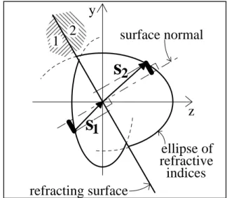
In case the optical axis of a uniaxially anisotropic substrate material lies in the plane of the waveguide (which is exclusively subject to my consideration here), the curve of (effective) refractive indices can be best approximated by an ellipse [56]. Fig. III.1 shows the connection between the directions of the wave vector and the ray vector in such an anisotropic medium. Fig. III.2 depicts the condition of phase matching for wave vectors at the border line (corresponding to a conventional refractive “surface”) of two adjacent anisotropic regions having different refractive indices.
y z
n
on
es
t
ellipse of refractive indices tangent to the ellipseFig. III.1. Connection between the wave vector s and the ray vector t in a two-dimensional medium of uniaxial anisotropy.
z y
s
1s
2 surface normal refracting surface 1 2 ellipse of refractive indicesFig. III.2. The condition of phase matching at a line separating uniaxial regions of different refractive indices (s1=incident wave vector, s2=refracted wave vector). 2.4 Model of in- and outcoupling
In this subsection, I overview the phenomena that served as a basis to my simple model developed for the purpose of optical design (see Section III.4). Detailed discussion about the the-oretical background of frustrated total internal reflection prisms can be found in [109], [106] and [66].
2.4.1 Incoupling of an infinite plane wave
The incident angle of an incoming plane wave must exceed the critical angle of total reflection at the waveguide/substrate interface, otherwise the wave refracts into the substrate. The mode-intensity vs. incident angle function has a local maximum in the waveguide, if the incident wave falls onto the waveguide surface in the so-called “synchronous direction” of a waveguide mode. In this case the condition of phase matching between the desired mode and the incident beam is fulfilled:
β
sin =
⋅ Θ
k , (III.1)
where k is the wave vector of the incident ray and β is the modified propagation constant of the waveguide mode. The propagation constant modification is a consequence of frustrated total reflection in the waveguide at its interface with the coupler prism. The narrower is the air gap (see Fig. III.3), the higher is the change in the propagation constant.
Due to the presence of the low refractive index region of the air-gap between the high-refractive index waveguide and the even higher index coupler prism, the different waveguide modes can be excited separately, with high intensity. The wider is the gap size, the smaller is the angle interval in which incoupling is possible (around synchronous directions). Since the air gap size can never decrease to zero, a small phase-shift also occurs when light traverses from the prism to the waveguide.
2.4.2 Incoupling of a “synchronised” beam of finite cross section
A collimated incident beam of finite cross section falling in according to a synchronised direction excites an exponentially increasing and then decreasing field in the waveguide (Fig. III.3). The limiting
value of mode intensity corresponds to the intensity excited by an infinite plane wave, see previous subsection. The field profile of the mode in the “Z” direction can be characterized by the coupling length (see Fig. III.3). The coupling length is by definition the distance, at which mode intensity increases to (1-1/e2) fraction of its maximum value at the beginning of the incident beam, and decreases to its 1/e2 fraction at the end of it. The coupling length increases exponentially (i.e. coupling becomes weaker) with gap size.
0 z Mode amplitude Coupling length 1. Air gap c. b. a. 2. 3. Illumination length
Fig. III.3. Field profile in the waveguide due to a collima-ted, finite incident beam. White arrows show energy propagation in the incident (1.), guided (2.) and reflected (3.) waves. (a. prism; b. waveguide; c. substrate.)
2.4.3 In- and outcoupling of a finite beam with a prism
If waveguide leakage is stopped at the end of the incident beam, the mode will propagate further in the waveguide without attenuation (neglecting losses caused by scattering on inhomogeneities etc.). This is satisfied if the incoming beam is positioned at the edge of the incoupler prism (see Fig. III.16).
Outcoupling takes place the opposite way (see Fig. III.4). As the mode reaches the edge of the outcoupler prism, its intensity gradually decreases to zero because of mode leakage. The mode profile in the “Z” direction will be the same as the decreasing part of an incoupled finite beam. The outcoupled beam is phase-matched to the waveguide mode. The small phase-shift through the air-gap and the propagation-constant modification here also occur.
2.5 Definition of “transverse inclination”
The image points formed by a waveguide lens are always situated on a single line in the case of a collimated input beam (see Fig. III.16). This is obvious, since the input beam direction can only be varied in 2D, i.e. in the plane of the waveguide (see integrated optical spectrum analyzers, beam deflectors [66]). According to former observations [106] and my calculations presented in Section III.4, the image line is not straight but curved if observed in air through an outcoupler prism. I call this phenomenon “transverse image line inclination”, which nomenclature intentionally implies that this effect is physically independent from the lens aberration known as curvature of field.
Phenomena behind transverse image line inclination can be traced back to the transverse inclination of single rays. To alleviate further explanations, I define “meridional planes” for the outcoupler prism (see Fig. III.4): a beam of parallel surface rays coupled out perpendicularly to the prism edge forms a plane in the prism and a plane in the air. I term these planes “meridional planes” because of their similarity to meridional planes used in classical geometrical optics. Surface rays that are not perpendicular to the prism edge cannot lie in the meridional plane after outcoupling (see Fig. III.4), i.e. they incline from it “transverse” direction. In case of single surface rays, I characterise transverse inclination by the distance between the outcoupled ray and the meridional plane, measured perpendicularly to the waveguide surface (see Fig. III.4). In case of beams, the displacement of the focus spot from the meridional plane in the air is of main interest. I describe the spot position by the transverse inclination of the ray that passes through its center (Fig. III.14 in Section III.5 was drawn in correspondence with this definition).
Surface ray of arbitrary direction
Surface ray (perpen-dicular to prism edge) Transverse inclination
Surface rays Meridional planes are perpedicular to the plane of paper
Side view Top view
O
O P
P
Fig. III.4. Explanation of meridional planes and definition of transverse image line inclination. Point “P” denotes intersection with prism edge, point “O” represents intersection with prism surface. (See also Fig. III.9 and Fig. III.10.)
3 Preliminaries (Former considerations concerning anisotropy and prism-outcoupled beams)
3.1 Introduction to anisotropic aberrations
Effects of optical anisotropy on the imaging properties of planar waveguide lenses have been investigated by several authors. These papers reveal large defocusing and focal spot deterioration (similar to spherical aberration) in optical systems designed with the usual approximation that characterise anisotropic lens materials with isotropic refractive indices. The main types of methods (all of which having some deficiencies) used for correction of anisotropic aberrations are listed below. a) The simplest way is to calculate analytically the necessary lens profile. Due to the approximations
incorporated, this is sufficient only for small field-angle 2D isotropic singlets [113, 111].
b) 3D design programmes (without modification) can simply treat 2D isotropic systems. In this way wide field-angle (aplanatic, etc.) lens systems can be designed [65, 84].
c) If anisotropy has to be taken into account, the designer must develop his own design software [56, 103]. The length of time required to write such a program is usually not acceptable.
d) Non-ray-tracing methods. Beam propagation methods [52, 79, 18] can analyze only low numeri-cal aperture lens systems with a narrow field-of-view, and they are also too slow for optimisation. 3.2 Outcoupling phenomena using coupler prisms
Certain papers investigating planar waveguides report that scattered light (always present due to waveguide inhomogeneities as well as surface defects) forms curved lines (each corresponding to one waveguide mode) after coupling a laser beam out of a waveguide using a coupler prism. These lines are known as m-lines, the curvature of which has not yet been explained. Experiments and calculations I made also supports the previous observation. In applications where a prism is used to couple out the image spots of a planar waveguide lens, the image line inclines just as m-lines of scattered light. As usually a CCD bar is used for the analysis of the outcoupled image, it is necessary to maintain straightness to avoid off-axis image spots wander off the CCD detector pixels.
4 Results (Efficient method to design waveguide lens systems, and their optimisation)
Since OSLO was written with three-dimensional optical elements in mind, it is not quite obvious how planar lenses should be modelled by the programme. For purely ray optical simulations one must trace rays only in one plane, however for diffraction analysis a planar lens must be replaced by a cylindrical one (because the wavefront leaving the exit pupil is always considered three-dimensional by commercial optical design programmes). The other difficulty arises from the fact that the built-in ray tracing routine of OSLO can use only one single refractive index per medium, so we must also adapt it for handling anisotropic media that have direction-dependent refractive index.
4.1 Building the model of anisotropy into OSLO SIX
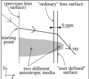
My aim was to solve anisotropic refraction/reflection at 2D surfaces of arbitrary shape, as well as to make as fast routines as possible. Therefore, I applied two coinciding surfaces instead of one User Defined Surface at each anisotropic lens surface (see Fig. III.5). These two surfaces consist of an ordinary lens surface (i.e. a conventional refractive surface) having the prescribed shape, and a User Defined Surface with the same profile. The distance between these surfaces are set to zero.
Ray-tracing is carried out in the following manner, regarding the path of a single ray started from the object point (Fig. III.5). The original OSLO algorithm first traces the ray to the first lens surface, which is an ordinary surface even in the case of an anisotropic medium. Hence, the intersection point coordinates are determined at the surface automatically by OSLO. These coordinates are then passed to my CCL routine at the User Defined Surface, which calculates the refracted ray directions together with the correct optical path and passes these back data to OSLO. After finishing it, OSLO continues to trace the ray towards the next lens surface. By application of two surfaces at the place of one anisotropic-to-anisotropic boundary I could economise on computation time by letting the fast built-in OSLO routine determine the intersection point of the ray and the surface, as well as the surface normal at this position. This way, my algorithm (run at the User Defined Surface) has to correct only the optical path, measured from the previous lens surface, and determine the direction of the refracted ray.
y z
(previous lens
surface) "ordinary" lens surface
"user defined" surface 0 mm two different anisotropic media ray starting point
Fig. III.5. Schematic view of a user defined surface and a ray.
The entry of an anisotropic waveguide lens begins with setting up the isotropic version of the lens system (using the extraordinary indices as refractive indices, as usual). To add the above-described User Defined Surfaces and to read-in the data that describe the anisotropic properties (e.g. the ordinary indices) of the lens, I wrote an auxiliary routine that performs these operations automatically, alleviating the designer’s task.
4.2 Modelling method of coupler prisms for optical design 4.2.1 Model of incoupling
Because of phase-matching, only those rays are allowed to couple into a waveguide, whose angle of incidence falls into a given interval around the synchronous direction of the selected mode. After a ray has been incoupled, it will propagate further as a surface ray in the plane of incidence (Fig. III.6). The criteria for coupling a ray into the waveguide are shown in Fig. III.8. Only those rays that hit the waveguide surface close to the prism edge are allowed to incouple. The distance limit is the coupling length. In the programme I realized this by placing a narrow aperture (i.e. a slit of size of the coupling length in “z” direction, and size of the input beam in “y” direction, see Fig. III.6) on the waveguide surface at the prism edge, parallel to the waveguide. Theoretically both the above mentioned angle interval and the coupling length could be calculated from the air-gap size (see Fig. III.3) and the refractive indices. However, as it is much more difficult to measure directly the refractive index and the air-gap size than the angle interval and the coupling length, these latter must be given to the programme by the user. Rays under the critical angle of total reflection are refracted into the substrate. The rest of the rays, those neither incoupled nor refracted into the substrate, are totally reflected on the prism base. The small phase shift between the incident beam and the excited mode (caused by the air gap) is neglected, since it is constant for each ray.
Waveguide Substrate User defined surface y z x
Fig. III.6. Coupling an incident beam into surface rays with a coupler prism. 4.2.2 Model of outcoupling
In my model all rays couple out at the line of the prism edge (see Fig. III.7) as if the coupling length were zero. The divergence angle of the outcoupled beam (in transverse direction to the waveguide plane) can be determined from diffraction on a coupling-length sized aperture (Fig. III.7). Outcoupled rays in the prism are phase-matched to the corresponding surface rays. The phase shift in the air gap is neglected as well as in the case of incoupling.
Waveguide Diffracted beam
Substrate User defined surface
Fig. III.7. Coupling out surface rays using a coupler prism. 4.2.3 Building the models into OSLO SIX
To calculate the intersection point of the incident ray at the waveguide surface, as well as the direction of the incoupled surface ray I place a User Defined Surface at the edge of the incoupler prism (Fig. III.6). The CCL routine at this surface follows the block diagram shown in Fig. III.8 to decide what to do with a particular ray (totally reflect, refract etc.). Another User Defined Surface is placed at the edge of the outcoupler prism (Fig. III.7) to determine the outcoupled ray direction.
The incident ray... ...hits the prism base? STOP at the prism edge. Incoupled ray. ...is in synchronous direction and within coupling length? Stop by total reflexion. STOP in the substrate. ...refracts into the substrate? Y Y Y N N N
Fig. III.8. Block diagram of the criterium system for incoupling a ray. 4.3 System design for reduced transverse image line inclination
“Transverse image line inclination” is a well-known effect, which has already been presented in [106], but it has not been explained yet. In this subsection I give the geometrical optical interpretation of this effect, and also show a method for its minimisation.
4.3.1 Geometrical optical interpretation – first approximation
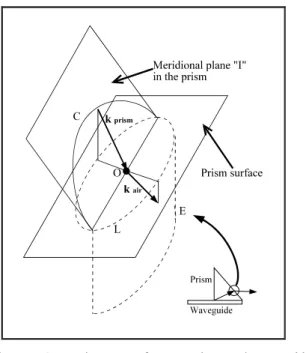
Below I prove indirectly that outcoupled rays of different direction cannot lie in the meridional plane in air, assuming that all the rays couple out of the waveguide into the prism in the meridional plane (see plane “I” in Fig. III.9). Let us suppose that the outcoupled rays pass through point “O” on the prism surface (Fig. III.9). From the law of refraction it directly follows that rays in the air must be phase-matched to the corresponding rays in the prism. In addition, the endpoints of all possible wave vectors kprism form a circle “C” in the prism. The orthogonal projection of this circle is an ellipse “L” on the prism surface. All the wave vectors in the air (kair) that are phase-matched to rays in the prism must be on a cylinder “E”, the cross section of which is ellipse “L”. On the other hand, the tips of the possible kair vectors form a sphere, the radius of which equals the length of the wave vector in air. Consequently, the refracted rays must be on the intersection curve of these two surfaces. If these rays were in the same plane, this curve would be a circle, but it is impossible, since cylinder “E” has only one circular cross section “C”, the radius of which equals the wave vector length in the prism. It is possible only in the case of normal incidence that all kair vectors lie in the meridional plane (i.e. when ellipse “L” reduces to a straight line).
Fig. III.9. Explanation of image line inclination (I). Outcoupled rays traverse from prism (kprism) to air (kair). 4.3.2 Geometrical optical interpretation – second approximation
In the previous subsection I assumed that all the outcoupled rays are in the meridional plane in the prism; now I examine the position of these rays in the prism, after outcoupling. For simplicity, let us suppose that all the surface rays pass through point “P”, situated on the prism edge “L” (see Fig. III.10). Since all these rays couple out under the same angle with respect to the waveguide plane (corresponding to the synchronous direction), the surface that these kprism wave vectors form in the prism is a cone, denoted by “K” in Fig. III.10. The assumption in the previous subsection that this surface can be approximated by a plane is thus strictly valid only for situations when the surface rays are nearly perpendicular to the prism edge. Although this is often the case, in reality the two effects shown above superimpose to determine the direction of outcoupled rays after the prism, i.e. in air.
Fig. III.10. Explanation of image line inclination (II). Surface rays (ββββ) couple out into the prism (kprism).
4.3.3 Minimising image line inclination
From Subsection III.4.3.1 it follows that the appropriate element for outcoupling would be a prism having a surface, which is perpendicular to the meridional plane in the prism (instead of the usually used 45° prism). However, according to Subsection III.4.3.2, outcoupling from the waveguide slightly changes the previously specified prism geometry. Since the prism surface can produce image line inclination in both up and down directions, by proper selection of the prism angle, the curve of the image line can be stretched into almost a straight line. The best prism shape can be detemined by automated optimisation (see Lens 3.3 in Subsection III.5.8). It must be noted here, that the optimal angle depends on, among other things, the waveguide effective index and the distance between the image and the outcoupler prism!
5 Application examples
In this section I present eight different waveguide lenses designed to work in different circumstances. Through these examples one can compare the changes in the operation of integrated optical lens systems if they are not used in that environment where they were designed to work (see also [103] and [1]). The main imaging properties of the lenses presented below are summarized in (Tab. III.1). Since these lenses were designed to work on a LiNbO3 substrate, the anisotropy is uniaxial and the optical axis lies in the plane of the waveguide (see Fig. III.16). The anisotropic effective refractive indices of the low-index and high-index waveguide regions are also listed in Tab. III.1 for the fundamental TE mode of the waveguide. All these lenses work at the vacuum wavelength of 632.8 nm and have a field angle of 2.5°. In each case when a coupler prism is used, only the prism angle α (see Fig. III.16) is changed; the prism base is 5 mm in length and the prism material is Bi12GeO20 with a refractive index of 2.55, in each arrangement.
Effective focal
length [mm] f-number (f#) Image NA ne / nLow index o
High index ne / no Lens 1.1 23.00 3.3 0.34 2.213 2.213 2.320 2.320 Lens 1.2 " " " 2.213 2.293 2.320 2.268 Lens 2.1 22.55 3.2 0.34 2.208 2.293 2.297 2.268 Lens 3.1 16.22 6.2 0.08 2.208 2.293 2.297 2.268
Tab. III.1. Main imaging properties of the discussed lenses and the effective refractive indices of the waveguide layers. 5.1 Lens 1.1: planar doublet in isotropic media
This doublet (Fig. III.11) was designed to work in an isotropic waveguide, without an outcoupler prism. The isotropic waveguide in this case is an approximation of the anisotropic LiNbO3 waveguide: the effective refractive index equals nextraordinary (for definition see Fig. III.16 and [54, 55, 115, 17]) in
every waveguide region, since the ordinary axis is perpendicular to the optical axis of the lens system. The lens was corrected to be diffraction limited in full image field by the usage of 10th order acircular surfaces [92, 103]. The focal properties can be read in Tab. III.2.
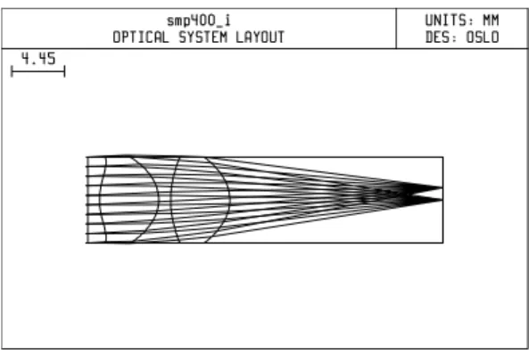
Fig. III.11. Layout of Lens 1.1. 5.2 Lens 1.2: planar doublet in anisotropic media
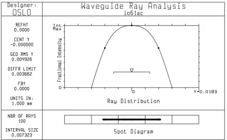
This lens contains the same surfaces as Lens 1.2 (i.e. it was not re-optimized), but the waveguide is now anisotropic. The effects of anisotropy can well be seen in the second line of Tab. III.2. It shows that anisotropy causes a huge focus shift (see “image distance”), and spoils the focus spot (see “RMS spot size” values and Fig. III.12).
Fig. III.12. On-axis spot diagram and ray distribution curve of Lens 1.2. (The symbol in the middle represents the centroid position and RMS size of the focus spot.)
5.3 Lens 1.3: planar doublet in anisotropic media with outcoupler prism
In this arrangement the outcoupler prism is also placed onto the waveguide surface of Lens 1.2; the prism angle is 45°. The result can be seen in the RMS spot size cells of Tab. III.2. The outcoupler prism acts like a plane parallel glass plate, since the outcoupled rays are almost in the same plane (see Subsection III.4.3). Consequently, the focus spots now contain a large spherical aberration.
Image distance [mm] On-axis RMS spot size [µm] Off-axis RMS spot size [µm] Airy radius [µm]
Max. image line inclination [µm]
Lens 1.1 18.00 0.1 0.2 0.9
Lens 1.2 19.51 10.3 14.7 0.9
Lens 1.3 (10.93) 42.1 99.1 0.9 7
Tab. III.2. Main focal properties of the doublet. 5.4 Lens 2.1: planar quadruplet in anisotropic media
This lens is a diffraction limited quadruplet, designed to work in an anisotropic waveguide (see Fig. III.13). The lens was corrected in full field using acircular surfaces of the 10th order. The focal properties are shown in Tab. III.3.
Fig. III.13. Layout of Lens 2.1. 5.5 Lens 2.2: planar quadruplet in anisotropic media with outcoupler prism
This is the same lens as 2.1 with the only difference that a 45° outcoupler prism is placed onto the waveguide surface. The large spherical aberration can well be seen again from the increment of the focus spot sizes in Tab. III.3.
On-axis RMS spot size [µm] Off-axis RMS spot size [µm] Airy radius [µm]
Max. image line inclination [µm]
Lens 2.1 0.2 0.7 0.9
Lens 2.2 3.3 4.0 0.9 0.1
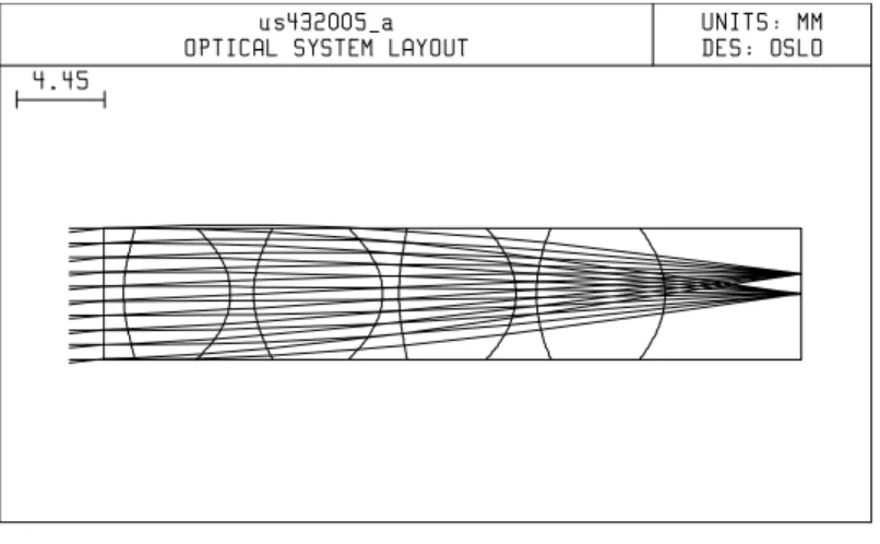
Tab. III.3. Main focal properties of the quadruplet. 5.6 Lens 3.1: planar singlet in anisotropic media with 45º outcoupler prism
This singlet (see lens in Fig. III.16) was designed to work in anisotropic waveguide in the presence of the outcoupler prism. Although it is a biconcave type lens, it focuses the light, since the low refractive index region is situated between the lens surfaces.