Hierarchical scene categorization : exploiting fused local & global features and outdoor & indoor information

(1)

Hierarchical Scene Categorization : Exploiting Fused

Local & Global Features and Outdoor & Indoor

Information

Thèse

Mana Shahriari

Doctorat en génie électrique

Philosophiæ doctor (Ph. D.)

(2)

Hierarchical Scene Categorization:

Exploiting Fused Local & Global Features

and Outdoor & Indoor Information

Thèse

Mana SHAHRIARI

Sous la direction de:

(3)

Résumé

Récemment, le problème de la compréhension de l’image a été l’objet de beaucoup d’attentions dans la littérature. La catégorisation de scène peut être vue comme un sous-ensemble de la compréhension d’image utilisée pour donner un contexte à la compréhension d’image ainsi qu’à la reconnaissance d’objet afin de faciliter ces tâches. Dans cette thèse, nous revisitons les idèes classiques de la catégorisation des scènes à la lumière des approches modernes. Le modèle proposé s’inspire considérablement de la façon dont le système visuel humain comprend et perçoit son environnement.

À cet égard, je soute qu’ajouter un niveau de classificateur extérieur – intérieur combiné à des caractéristiques globales et locales de scène permet d’atteindre une performance de pointe. Ainsi, un tel modèle requiert ces deux éléments afin de gérer une grande variété d’éclairage et points de vue ainsi que des objets occultés à l’intérieur des scènes.

Le modèle que je propose est un cadre hiérarchique en deux étapes qui comprend un classifica-teur extérieur – intérieur à son stade initial et un modèle de scène contextuelle au stade final. Je monte ensuite que les fonctionnalités locales introduites, combinées aux caractéristiques glo-bales, produisent des caractéristiques de scène plus stables. Par conséquent, les deux sont des ingrédients d’un modèle de scène. Les caractéristiques de texture des scène extérieures agissent comme caractéristique locale, tandis que leur apparence spatiale agit comme caractéristique globale. Dans les scènes d’intérieur, les caractéristiques locales capturent des informations détaillées sur les objets alors que les caractéristiques globales représentent l’arrière-plan et le contexte de la scène.

Enfin, je confirme que le modèle présenté est capable de fournir des performances de pointe sur trois jeux de données de scène qui sont des standards de facto; 15 – Scene Category, 67 – Indoor Scenes, et SUN 397.

(4)

Abstract

Recently the problem of image understanding has drawn lots of attention in the literature. Scene categorization can be seen as a subset of image understanding utilized to give context to image understanding also to object recognition in order to ease these tasks. In this thesis, I revisit the classical ideas, model driven approaches, in scene categorization in the light of modern approaches, data driven approaches. The proposed model is greatly inspired by human visual system in understanding and perceiving its environment.

In this regard, I argue that adding a level of outdoor – indoor classifier combined with global and local scene features, would reach to the state-of-the-art performance. Thus, such a model requires both of these elements in order to handle wide variety of illumination and viewpoint as well as occluded objects within scenes.

The proposed model is a two-stage hierarchical model which features an outdoor – indoor classifier at its initial stage and a contextual scene model at its final stage. I later show that the introduced local features combined with global features produce more stable scene features, hence both are essential components of a scene model. Texture-like characteristics of outdoor scenes act as local feature meanwhile their spatial appearance act as the global feature. In indoor scenes, local features capture detailed information on objects, while global features represent background and the context of the scene.

Finally, I have confirmed that the presented model is capable of delivering state-of-the-art performance on 15 – Scene Category, 67 – Indoor Scenes, and SUN 397, three de-facto standard scene datasets.

(5)

List of Tables

1.1 Comparison between three main approaches i.e. region and shape based

tech-niques, deep scene features, and bag of visual words in scene categorization. . . 53

2.1 The scene categorization performance on 15 – Scene Category dataset. LLC represents the results without considering background or contextual features whereas CLBP + LLC represents the results with the proposed CSI model. For all the results, the value of Threshold is fixed and is T = 5 × 10−3. For

single-level CLBP parameters, (P,R) pair are set to (8,1). . . 70

3.1 The categorization performance and the percentage increase of 15 – Scene Cat-egory dataset. LLC represents the results without considering background fea-tures. CLBP + LLC reports the results with the proposed CSI model when considering both foreground and background features. Living Room category stands at the highest with 24% increase in performance. Forest category stands

at the lowest with 0.31% percentage increase. . . 72

4.1 Confusion Matrix of the proposed HOI model on 15 – Scene dataset, having the Industrial category considered as an indoor scene. The entry located in ith row and jthcolumn in confusion matrix represents the percentage of scene category

i being misclassified to scene category j. . . 90

4.2 Confusion Matrix of the proposed HOI model on 15 – Scene dataset, having the Industrial category considered as an outdoor scene. The entry located in ith row and jth column in confusion matrix represents the percentage of scene

category i being misclassified to scene category j. . . 90

4.3 The overall performance of the proposed HOI + CSI model on 15 – Scene Category with respect to threshold T. LLC presents the performance in the absence of contextual or background features. Whereas LLC + CLBP presents the performance in the presence of both foreground and background features. To report results on LLC encoding, we have used 16384 visual words. For the proposed CSI model, we have used both single-level and multi-level CLBP analysis, i.e CLBP8,1+16,2+24,3. In addition Industrial class is taken as an Indoor

category.. . . 92

4.4 Final categorization results on 15 – Scene Category dataset using the proposed HOI + CSI model. The threshold value for experiments in this table is T = 7.5 × 10−3. Also the codebook size on high-contrast regions is 4096 and the

(8)

4.5 The overall performance of our proposed model on 67 – Indoor Scenes with respect to threshold T. LLC presents the performance in the absence of the contextual or background features. LLC + CLBP presents the performance in the presence of both foreground and background features, i.e. the proposed CSI model. For the proposed CSI model, we have used both single-level and

multi-level CLBP analysis i.e. CLBP_{8,1+16,2+24,3}. . . 98

4.6 Final categorization results on 67 – Indoor Scenes dataset using the proposed CSI model. The threshold value for experiments in this table is T = 5 × 10−3. Also the codebook size on high-contrast regions is 8192, and the multi-resolution

CLBP scheme CLBP_{8,1+16,2+24,3} is applied. . . 98

4.7 The performance of the proposed HOI model over 221 scene categories of SUN397 dataset. The names in the table are sorted in alphabetical order. Note that, the performance is reported at 16K codebook size for this datasets,

with 21 SPM regions. . . 105

4.8 Final categorization results on SUN 397 dataset using our proposed HOI + CSI model. The threshold value for experiments in this table is T = 5 × 10−3. The codebook size on high-contrast regions is 8192, and the multi-level CLBP

scheme CLBP8,1+16,2+24,3 is applied. . . 107 4.9 The overall performance of our proposed model on SUN 397 with respect to

threshold T. LLC presents the performance in the absence of contextual or background features. LLC + CLBP presents the performance in the presence of both foreground and background features i.e. the proposed CSI model. To report results on LLC encoding, we used both single-level and multi-level CLBP

analysis i.e. CLBP8,1+16,2+24,3. . . 107 5.1 Brief comparison of engineered or handcrafted features driven by model driven

approaches and deep features driven by data driven approaches for the scene categorization problem. There is a tradeoff between the performance of deep networks and robustness, simplicity, and interpretability of engineered features

(9)

List of Figures

0.1 Eight examples of outdoor scene categories. The labels from left to right and top to bottom are Inside City, Broadleaf Forest, Desert, Lake, Snowy Mountain,

Hay Field, Butte, and Strait. . . 2

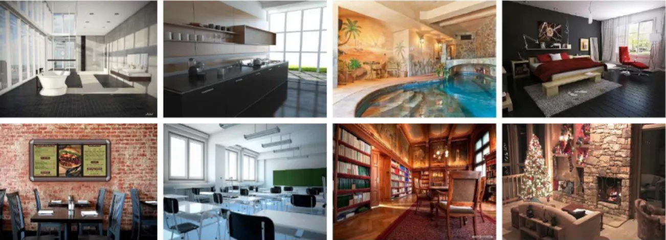
0.2 Eight examples of indoor scene categories. The labels from left to right and top to bottom are Bathroom, Kitchen, Swimming Pool, Bedroom, Restaurant,

Classroom, Library and Living Room. . . 2

0.3 The story that this image is telling is known as scene understanding (photo

credit Twitter) . . . 3

0.4 The main components of scene understanding. The image is reproduced from

[Balas et al., 2019]. . . 5

0.5 The relation between scene categorization and other domains. Scene

catego-rization can be used to ease these tasks by giving context to them. . . 7

0.6 An example of a scene with removed objects. Even though objects are removed, the perception of this scene is complete which comes from surfaces, line distri-butions, textures, and volumes. The photo is taken from [Biederman et al.,

1982] . . . 10

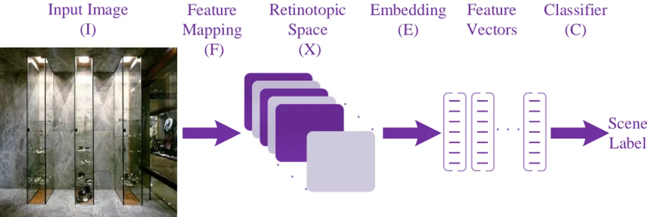
1.1 The general architecture of a scene categorization model is presented here. The input image is first mapped to a retinotopic space (X). Later, the feature vectors are built by embedding the representations in X space. The final step is the classifier C which classifies the feature space to have a scene label as the final

output of the algorithm. The idea is adopted from [Dixit et al., 2015]. . . 16

1.2 The general flowchart of a Bag of Visual Words (BoVW) framework. It starts by extracting several key-points (patches) from an input image, follows by describ-ing and clusterdescrib-ing them into the codebook. The final image-level representation is obtained by pooling the coding coefficients of encoded local descriptors. The

idea is adopted from [Huang et al., 2014]. . . 18

1.3 Harris corner detector: classification of image points using eigenvalues of M . . 20

1.4 An example of a living room scene and some of the detected Hessian interest

points. . . 21

1.5 Estimating Laplacian of Gaussian with difference of Gaussian). The image is

adopted from [Lowe, 2004] by David Lowe.. . . 23

1.6 An example of a living room scene and some of the detected Difference of

Gaussian interest points. . . 24

1.7 An example of a living room scene and some of the detected Harris Laplacian

interest points. . . 25

1.8 An example of a living room scene and some of the detected Hessian Laplacian

(10)

1.9 An example of a living room scene and some of the detected Estimated Affine

Covariate Shape interest points.. . . 28

1.10 An example of a living room scene and some of the Dense interest points. . . . 30

1.11 An example of a living room scene and some of the Random interest points. . . 31

1.12 SIFT key-point descriptor calculated over 4×4 image subregions. The descriptor proposed by David Lowe is computed over 16 × 16 set of samples. The image

is adopted from [Lowe, 2004] by David Lowe. . . 33

1.13 The main building blocks of a Convolutional Neural Network (CNN). The ar-chitecture has three main components; convolutional layers, pooling layers, and

fully connected layers. The image is taken from [Murugan, 2017]. . . 41

1.14 An illustration of the architecture of AlexNet. The network’s input is 150,528-dimensional, and the number of neurones in the network’s remaining layers is 253,440 - 186,624 - 64,896 - 64,896 - 43,264 - 4096 - 4096 - 1000. The image is

taken from [Andrew Ng, Kian Katanforoosh, Younes Bensouda Mourri, 2017]. . 42

1.15 96 convolutional kernels of size 11 × 11 × 3 learned by the first convolutional layer on the 224 × 224 × 3 input images. The filters are taken from AlexNet [Krizhevsky et al., 2012] on ImageNet dataset [Deng et al., 2009, Russakovsky

et al., 2015]. . . 45

1.16 Diagram of three possibilities of transfer learning form a pre-trained CNN model. From left to right fixed feature extractor, fine-tuning, and initializa-tion techniques are shown. The diagram is taken from [Khademi and Simon,

2019]. . . 46

1.17 With only one example, a human observer can say pretty easily which one of these is character 1 and which one is character 2. This ability, however, is not affected by how the handwritings differ, how complex the characters are, and where the characters appear in the image. The image is taken from a research

by [Lake et al., 2015]. . . 48

1.18 Data augmentation of a cat image. The image is taken from a review by

[Gandhi, 2018]. . . 49

1.19 Sample images from Syn2Real dataset [Peng et al., 2018]. The top two rows are source images synthetically rendered; the middle two rows are validation target images cropped from COCO dataset [Lin et al., 2014b] and the last two rows

are test target images cropped from YouTube-BB dataset [Real et al., 2017]. . . 50

2.1 The general flow chart of the proposed modelling approach. The model is built on the idea of BoVW; it starts by extracting key-points and describing them. Later the feature vector is formed by encoding descriptors. In our proposed model, foreground and background features are encoded separately and are

fused to form the final image-level representation. . . 56

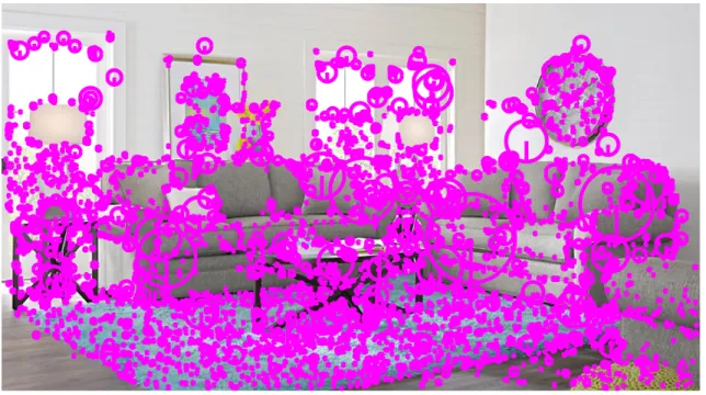
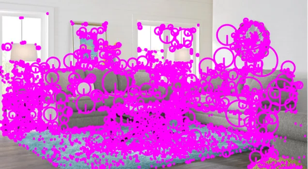
2.2 Visualization of regions with non-stable Dense SIFT descriptors with regions whose norm is smaller than Threshold T (kxnk ≤ T ). Two sample images from 15 – Scene Categories, from ‘Open Country’ and ‘Store’ classes are chosen. ‘Open Country’ belongs to an outdoor scene whereas ‘Store’ belongs to an indoor class. For a better visualization of these regions we only plotted them in one scale and the sampling step of dense features is set to be equal to double

(11)

2.3 Visualization of regions with non-stable Dense SIFT descriptors with regions whose norm is smaller than Threshold T (kxnk ≤ T ). Two sample images from 67 – Indoor Scenes, from ‘Hair Salon’ and ‘Closet’ classes are chosen. Both ‘Hair Salon’ and ‘Closet’ belong to an indoor scene. For a better visualization of these regions, we only plotted them in one scale and the sampling step of

dense features is set to be equal to double the spatial grid of SIFT features. . 59

2.4 Visualization of regions with non-stable Dense SIFT descriptors with regions whose norm is smaller than Threshold T (kxnk ≤ T ). Two sample images from SUN397 dataset, from ‘Chalet’ and ‘Dorm Room’ classes are chosen. ‘Chalet’ belongs to an outdoor class whereas ‘Dorm Room’ is an indoor scene. For a better visualization of these regions, we only plotted them in one scale and the sampling step of dense features is set to be equal to double the spatial grid of

SIFT features. . . 60

2.5 Contextual or background features extraction as proposed in this thesis. Non-stable regions i.e. low-contrast regions are encoded to represent features on

background regions or f_B (see Equation 2.1). . . 61

2.6 The general flowchart of the proposed modelling approach when descriptors form stable regions (X_High) and non-stable regions (XLow) are encoded in a

local and global manner respectively. . . 62

2.7 The general flowchart of the proposed modelling approach. Global and local

scene features are concatenated to form the final image-level representation. . . 64

2.8 Flowchart of LLC encoding process. The image is reproduced from [Wang et al.,

2010]. . . 65

2.9 Flowchart of CLBP coding. The image is reproduced from [Guo et al., 2010]. . 66

2.10 The general flowchart of the proposed Contextual Scene Information approach

when XHigh is encoded by LLC and XLow is encoded by CLBP. . . 67 3.1 Visualization of sample images from scene categories of Coast, Highway, Inside

City, Mountain, Open Country, Street, Suburb and Tall Building. Background regions for the threshold value of 5 × 10−3are depicted. For all these categories, the CSI model has not shown a significant improvement in performance. The categorization performance has shown an improvement of less than 2% in these

categories when the CSI model is employed. . . 74

3.2 The general scheme of our proposed Hierarchical Scene Classification (HSC) model. As the model suggests in the first stage, we do not have a binary

classifier, rather several outdoor scene labels in addition to the indoor label. . . 75

3.3 The general scheme of our proposed model for Outdoor – Indoor classification. We use both global and local features to in order to classify the indoor and

outdoor labels. . . 77

3.4 The 40 Gabor-Wavelet filters used in this thesis. Three are in 5 scales (equally spaced from 0 to π) and in 8 orientations, and are l1 normalized for scale

invariance.. . . 79

3.5 The detailed flowchart of building the visual words along with building scene models. Any of the model descriptors are assigned to the closest visual word which is obtained by clustering training descriptors. The final scene models are

(12)

3.6 Toy example of constructing a three-level spatial pyramid. Three types of fea-tures are shown in the image. For different spatial regions, the number of each type of feature is counted. The distribution histograms are collected according to the weight. The final histogram is concatenation of histograms from each

spatial region. The image is reproduced from [Lazebnik et al., 2009]. . . 81

3.7 The detailed flowchart of the Outdoor – Indoor model and how local and global

features are fused to form the final image-level representation. . . 82

3.8 The detailed flowchart of the Hierarchical Outdoor – Indoor (HOI) scene

cate-gorization model proposed in this Chapter. . . 83

3.9 The detailed flowchart of our scene categorization model (HOI+CSI). The model itself consists of two main blocks; (i) a hierarchical classifier for classifying all outdoor labels vs. one indoor class, which incorporates both local and global features (green flowchart) (ii) categorizing indoor classes by encoding high-contrast regions using LLC as local features and low-high-contrast regions using

CLBP as global features (blue flowchart). . . 84

4.1 15 example images from 15 – Scene Category dataset in alphabetical order. One sample image from each class is selected. The dataset includes 9 outdoor scene categories which are Suburban, Coast, Forest, Highway, Inside City, Mountain, Open Country, Street, and Tall Buildings; 5 indoor scene categories which are Kitchen, Bedroom, Living Room, Office, and Store; and 1 category of mixed

indoor and outdoor images which is Industrial. . . 88

4.2 Classification performance of the proposed HOI model on 15 – Scene Category when varying the size of codebook. The size of codebook varies from 16 to 16384 for this dataset, and 8 SPM regions are used. The results are reported as the mean and standard deviation of the performance from running the experiment

for 10 individual times. . . 92

4.3 Categorization performance of the proposed CSI model on 15 – Scene Cate-gory when varying the size of codebook from 16 to 16K on high-contrast re-gions. The number of neighbours and the radius of neighbourhood for single-level CLBP are set to (8,1),(16,2),(24,3). The results on multi-level CLBP i.e. CLBP_{8,1+16,2+24,3} is also provided. The threshold value is fixed to be T

= 7.5 × 10−3 in this table. . . 94

4.4 21 example images from 67 – Indoor dataset in alphabetical order. Since there exists 67 classes in the dataset, only one sample category from each letter of

alphabet is selected. . . 96

4.5 Summary of 67 – Indoor Scenes; the dataset is divided into 5 scene classes:

Store, Home, Public Spaces, Leisure, and Working Place.. . . 97

4.6 Categorization performance of the proposed CSI model on 67 – Indoor Scenes when varying the size of codebook from 16 to 16K on high-contrast regions. The number of neighbours P and the radius of neighbourhood R in CLBP are set to (8,1),(16,2),(24,3). In addition, the results on multi-resolution CLBP is provided here. For a better understanding of the results, the threshold value is

fixed to T = 5 × 10−3. . . 99

(13)

4.8 23 example images from SUN 397 dataset in alphabetical order. Due to the extensive number of classes in the dataset, only one sample class from each letter of alphabet is chosen. There exists 220 outdoor categories, 175 indoor

categories and 2 categories with the mixed outdoor and indoor images. . . 102

4.9 Classification performance of the proposed HOI model on SUN 397 Category when varying the size of codebook. The size of codebook varies from 16 to 16384 for this dataset and 21 SPM regions are used. The results are reported as the mean and standard deviation of the performance from running the experiment

for 10 individual times. . . 104

4.10 Selected outdoor scene classes from SUN 397. The top two row are classes with the highest performance and the two bottom rows are classes with the least performance. Column (A) shows samples of training images for each class, (B) the correctly classified images, (C) the examples of images from other classes falsely labeled as true, and finally (D) the examples of test images from each of

the corresponding classes that are predicted with the wrong label.. . . 105

4.11 Categorization performance of the proposed CSI model on SUN 397 when vary-ing the size of codebook from 16 to 16K on high-contrast regions. The number of neighbours P and the radius of neighbourhood R in CLBP are (8,1), (16,2), (24,3). In addition, the results on multi-resolution CLBP is given. The

thresh-old value is fixed to T = 5 × 10−3. . . 108

5.1 The left image shows real graffiti on a Stop Sign, something that most humans would not think is suspicious. The right image shows a physical perturbation applied to a Stop Sign. The systems classify the sign on the right as a Speed

Limit: 45 mph sign. Image is taken from the research by [Brown et al., 2018]. . 114

5.2 As a future work and in order to overcome the shortcomings of BoVW and CNN, we can fuse engineered features and deep scene features for scene categorization.

(14)

List of Abbreviation

BoVW Bag of Visual Words

CLBP Completed Local Binary Pattern CNN Convolutional Neural Networks CSI Contextual Scene Information HOI Hierarchical Outdoor Indoor HSC Hierarchical Scene Classification LLC Locality-constrained Linear Coding SIFT Scale-Invariant Feature Transform SVM Support Vector Machines

(15)

To Babayi, my first man, my lifelong mentor, my hero, and my friend, whose world was immense though the world was too tiny for him. This thesis is dedicated to the memory of an outstanding and big hearted dad whose lose left a huge scar in my life. Sadly he could not stay long enough to see it completed ...

(16)

A picture is worth a thousand words.

(17)

Acknowledgments

It is a pleasure to thank those who made the completion of this thesis possible. A sincere thank you to my supervisor, Professor Robert Bergevin, who gave me invaluable assistance, advices, and ideas. He was not only a supervisor to me, he was supportive, patient, compassionate, and taught me precious life lessons.

Special thanks to all members of Laboratoire de Vision et Systèmes Numériques de l’Université Laval (LVSN), to Annette Schwerdtfeger and Denis Ouellet for their helping attitude and supports. It was a great experience and my pleasure to be part of them. My gratitutes to other members of département de génie électrique et de génie informatique (GEL-GIF), Nancy Duchesneau and André Desbiens in particular. Nancy, you have always been there with a big smile on your face; helping me, answering my questions, solving my issues or anything that could concern me. André, you saved me.

I would also like to take this opportunity to thank many individuals for their help, guid-ances, motivations, and encouragements throughout my graduate studies. Abhichek, Arsene, Atousa, Azadeh, Brooke, Farnoosh, Hassan, Julien, Karen, Keyhan, Kyarash, Lyn Yan, Mo-jgan, Najva, Negar, Nivad, Reyhaneh, Saara, and Soroosh; this thesis would have not been accomplished without the help and support from you. My deepest gratitude to Mamany and Babayi, my main supporters and incentives, for their unconditional love and ongoing support, you raise me up to more than I could be. I am blessed to have so many amazing people in my life. If it was not because of you, I would have not been here. I could not be more grateful, you are the most valuable things I have in my life.

Last but not least, I appreciate all the moments and the experiences I have had during my PhD. This was a journey with lots of ups and downs, it had happy and sad moments, it was satisfying yet not easy, it was fantastic and at the same time tough. It was not only a professional journey, but a self-discovery journey. It was a life lesson I learnt at an expensive price, but it definitely worthen it. I do believe PhD studies gave me capabilities and the mindset of becoming a better version of myself. Yes, it was a fulfilling journey, an amazing experience, it had little bit of everything in it, and I enjoyed every bit of it. And now at the very end of this journey I am holding my head up high; I am happy I did it for myself and I am so proud of myself.

(18)

Introduction

We present in this thesis a hierarchical approach for scene categorization based on computer vision techniques. Before entering technical details, we first review scene categorization defi-nitions to explain what our motivations are and how we are inspired to develop the proposed method. In which follows, we start by providing a general overview and description for human vision, computer vision, and scene understanding. We continue then with further discussions on objects, scenes, and scene perception from human perspective as we use it through the context of this thesis. We then briefly explain the existing scene categorization approaches in computer vision the respective shortcomings. We finally define the general and specific objectives, the proposed methodology, and describe the outline of the following chapters.

Scene Understanding in a Human Vision Context

Vision is a process that produces, “from images of the external world, a description that is useful to the viewer and not cluttered with irrelevant information” [Marr and Nishihara, 1978]. It is effortless for humans to understand the three-dimensional structure of the world with apparent ease. In other words, they can perceive the world through noise, shadows, color variations, depth and motion ambiguities.

Given an arbitrary photograph or picture we first would like as a human to describe what scenes are. Scenes are described in the literature as the views of the world. Scenes refer to a set of environments that share visual similarities which may lead to similar interactions and activities. Scene can also be the answer to the question “I am in the place”, or “Let’s go to the place”. Sometimes, scenes are defined by objects. Nevertheless, objects are compact and acted upon, whereas scenes are extended in space and acted within [Xiao et al., 2014]. Hence, unlike objects, scenes do not necessarily have clear segmentable boundaries. Figures 0.1and

0.2 depict some examples of scenes from outdoor and indoor classes respectively.

Scene understanding on the other hand is recognizing the complex visual world and describing what is happening in the image [Torralba and Sinha, 2001, Brandman and Peelen, 2017, Li and Fei-Fei, 2007]. In scene understanding, we want to know what the image is about and what story it is trying to tell; it is telling the what, where, and who the story behind an image

(19)

Figure 0.1: Eight examples of outdoor scene categories. The labels from left to right and top to bottom are Inside City, Broadleaf Forest, Desert, Lake, Snowy Mountain, Hay Field, Butte, and Strait.

Figure 0.2: Eight examples of indoor scene categories. The labels from left to right and top to bottom are Bathroom, Kitchen, Swimming Pool, Bedroom, Restaurant, Classroom, Library and Living Room.

is about.

Every story occurs in a context. This is known as the category or the label of scene. Then comes the characters such as people, animals, robots, and things. These are known as the objects in the scene. Next, is the relationship between the objects with respect to each other and the scene category. This is known as the actions of a scene. Actions themselves can lead to events which are the collection of actions. We can go further than this and finish the story by describing the feeling and thoughts of a person into it. This is known as understanding the scene.

An example of a scene understanding process is given in Figure 0.3. In this figure, the story happens in a rural area (the scene category). The characters of the scene are young kids (the

(20)

Figure 0.3: The story that this image is telling is known as scene understanding (photo credit Twitter)

objects). These kids are standing, smiling, and one is holding a rubber slipper in his hand (the actions). These children, five to be specific, are posing for a selfie (the event). However, this is not the end of the story. This selfie does not involve a camera or smartphone. This photo can be a set-up by a thoughtful mind behind the camera which helped us to see the actual photo (scene understanding). Some other thoughts that may be noticed is that four of these kids do not have slippers on their foot. Only one of them had one which he is using to take the selfie.

Scene understanding exists on a continuum; at one end it is a very fast and seemingly effortless extraction of scene category or label names. At the other end, it is the slower and often effortful attachment of deeper meaning to the scene i.e. understanding it [Zelinsky, 2013]. Scene understanding can also be defined as predicting the scene category, scene attributes, the 3D enclosure of the space, the objects in the image, and whether there is text in the image and how this text is related to other objects of the image.

(21)

Scene Understanding in a Computer Vision Context

Many efforts have been made to make computers the powerful tools to simulate and eventually imitate some of the human capabilities. The main motivations, depending on the context, could be speed and discharge of the labor force from repetitive and tiresome tasks, eliminate human-to-human bias in processing data, uniformity, and repeatability in results. The main enablers in this regard is the ever-increasing connectivity and processing capabilities with less costs.

Humans acquire most of their daily information from their visual system. Thus, many re-searches have been made in (i) understanding the process of visual understanding in humans and (ii) imitating this procedure by computers. This is known as computer vision. Com-puter vision is an interdisciplinary scientific field which involves comCom-puter science, artificial intelligence, neuroscience, psychology, applied mathematics, physics, engineering, philosophy, art, etc. It seeks two goals; one from biological point of view and one from engineering and computer science point of view:

i Studying biological vision requires an understanding of the perception organs like the eyes, as well as the interpretation of the perception within the brain [Szeliski, 2010]. Accordingly, from biological point of view computer vision aims at coming up with computational models of the human visual system [Huang, 1996].

ii From the engineering and computer science perspective, we seek to automate tasks that the human visual system can do. Thus, from this point of view, the goal is building autonomous systems that attempt to reproduce the capability of human vision.

Both of these goals are related i.e. properties and characteristics of the human visual system often give inspiration to engineers who are designing computer vision systems. Conversely, computer vision algorithms can offer insights into how the human visual system works [Szeliski, 2010].

It is well known that humans can perceive and understand a scene quickly and accurately with little or no attention [Fei-Fei et al., 2007]. This is true even under poor viewing conditions such as brief exposure duration, dim lighting, and biasing the image by adaptation of noise [Kaping et al., 2007]. Given the fact that scene perception is effortless for most human observers, it might be thought of as something easy to understand. However, the exact nature of the processes involved in scene perception is still largely unknown in human vision.

Compared to human vision and perception, scene understanding has introduced unique chal-lenges to computer vision and remains limited in terms of accuracy and performance. The main difficulty arises from the fact that computers inherently work well to solve tightly con-strained problems, not open unbounded ones like visual perception as we know it from human

(22)

Scene

Understanding

Visual Question Answering Face Recognition Scene Categorization Caption Generation Depth Estimation Object Recognition Scene Text Detection

Figure 0.4: The main components of scene understanding. The image is reproduced from [Balas et al., 2019].

perspective [Brownlee, 2019]. Based on what we explained up to now, by seeing one does not mean to simply record images and pictures, but rather to detect objects, detect relationships between the objects, understand the scene and comprehend the context or in other words, to convert pictures and images into information and knowledge. Scene understanding is telling the story that is attached to a collection of pixels.

From the provided definitions, scene understanding process can be split and broken into its building components that are namely object recognition, scene text detection, depth map estimation, face detection and recognition, scene categorization, caption generation, and visual question answering (Figure0.4). These components are inter-connected and form the essential elements in the framework for complete understanding of a scene [Balas et al., 2019]. We focus, in the following, on scene categorization as the subject under study in this research thesis as a building block in scene understanding with diverse applications in forthcoming emerging technologies based on computer vision technology.

Scene Categorization as a Driving Factor in Scene

Understanding

Due to the importance of scene categorization in scene understanding, many researchers have actively been working on this topic for the past twenty years such as CSAIL at MIT, Prince-ton Computer Vision and Robotics Labs, Stanford Vision and Learning Lab, Inria Grenoble

(23)

Rhone-Alpes. In scene categorization, we aim at determining and attributing the content labels that describe a given image which are called scene labels.

For both humans and machines, the ability to learn and categorize scenes is an essential and important functionality. Torralba and Sinha [Torralba and Sinha, 2001] argued that scene categorization can be seen as the first step in scene understanding. Let’s then take one step back and revisit scene definition from another angle. A “scene” in the dictionary is defined as “the place where an incident in real life or fiction occurs or occurred, a landscape, an incident of a specified nature” [Stevenson, 2015]. By scene we mean a place in which a human can act within, or a place to which a human being could navigate [Xiao et al., 2014]. Scene perception and categorization is not trivial for humans, as it is the “gateway to many of our most valued behaviors, like navigation, recognition, and reasoning with the world around us” [Xiao et al., 2010]. The same strains can easily be extended to machines and in computer vision context. Scene categorization is therefore defined as the semantic category of an image also known as scene labels (see Figures 0.1 and 0.2). This definition is valid for both human and computer vision. The goal of scene categorization in computer vision is to make machines perform like humans i.e. to understand the semantic context of visual scenes. In this context, scene categorization algorithms aim at analyzing the content of an image and label it among a set of semantic categories automatically. A scene category is more than only a label and it mostly comes in bundled with expectations of objects, locations, events, etc. Some of the related fields to scene categorization in computer vision can be named as (see Figure 0.5):

i Scene Graph Scene categorization can be seen as a subset of scene graph [Chen et al., 2019, Gu et al., 2019]. In scene graph, the goal is describing what is happening in the image, what are the elements of the image and its content, and how do they relate to each other. In constrained environments where an image belongs to one of the considered classes, image features can be used to distinguish between conceptual image classes [Brandman and Peelen, 2017, Gu et al., 2019]. However, scene graph in unconstrained environments remains an open and challenging issue in computer vision.

ii Autonomous Driving & Indoor Positioning and Navigation Scene categorization provides imperative and complementary information for simple interactions such as nav-igation and object manipulation. Scene detection is also used for visuo-motor operations such as reaching or locomotion and accurate localization for indoor and outdoor position-ing. For an intelligent system, which is navigating in an environment, knowing the place it is located and the place in which main objects appear in the scene is very important. Knowing the place improves the decision-making process for further actions. Knowing the scene helps the autonomous agent to understand what might have happened in the past and what may happen in the future. It also helps to understand the cause of events [Xue et al., 2018].

(24)

Scene

Categorization

Object Recognition Autonomous Driving Indoor Positioning & Navigation Event Description Surveillance Application Image Enhancement Scene Graph

Figure 0.5: The relation between scene categorization and other domains. Scene categorization can be used to ease these tasks by giving context to them.

iii Object Recognition Another key feature of scene categorization is to assist in identifying possible and realistic locations for each of the objects in an image or a picture [Lauer et al., 2018]. The scene category provides an appropriate level of abstraction for the recognition system to improve the performance for rapid recognition and segmentation of objects in addition to spotting inconsistent objects in the picture. Given the scene category, the system can avoid going through long and complex list of objects and a description of their spatial relationship [Zhou et al., 2014, Henderson, 1992]. Thus, objects that are semantically related to their scene context are detected faster and more accurately than objects that are unpredicted by the context [Biederman et al., 1982]. Also, an object within a semantically related scene is recognized more quickly than the same object presented in a semantically unrelated scene.

iv Surveillance Application and Event Description Like objects, particular environ-ments will trigger specific actions such as eating in a restaurant, drinking in a pub, reading in a library, and sleeping in a bedroom [Li and Fei-Fei, 2007, Xiao et al., 2010]. Thus, depending on the specifics of the place, we would act differently. This is critical for artifi-cial vision systems to discriminate the type of environments at the same level of specificity as humans [Xiao et al., 2014]. As it helps to determine the actions happening in a given environment, also to spot inconsistent human behaviors for a particular place.

(25)

context-sensitive image enhancement, augmented reality applications, detecting image orien-tation, optimizing the shutter speed, aperture, brightness and contrast to best suit scenes in digital cameras, image retrieval, and intelligent image processing systems. The main goal of scene categorization would then be the establishment of a stable context for various aspects of visual processing such as object recognition, event classification, and scene graph.

Object Recognition, Scene Categorization, and Scene

Perception

Before describing the problem statement in the context of this thesis let’s revisit the definition of “scene” and its relation to “object”. We call a scene, a meaningful and realistic composi-tion of a series of objects which can vary in pose, illuminacomposi-tion, and occlusions, arising from other objects or from cast shadows. Although we can think of scenes as distinct combina-tions of objects, we should also note that there are far fewer scene categories than there are possible combinations and configurations of objects. This is because not all distinct object configurations give rise to different scene categories [Zhou et al., 2014,Xiao et al., 2014]. An example is a bedroom scene with different bed types, curtains, or decorations. Meanwhile, some objects are crucial for categorizing scenes for instance a bed for a bedroom and paintings for art gallery. These objects are referred to as informative objects in the literature [Cheng et al., 2018]. Contrarily to informative objects, some other objects can be removed from scenes without affecting their meaning. Examples are birds flying in a sunset scene or a towing and transportation trucks in an airport scene (see Figure 0.6).

Experiments on humans based on naming and categorization of images also confirms that a small set of objects and scene properties is enough to provide us, as humans, with scene perception and categorization process. During a rapid sequential visual presentation (less than 150 milliseconds per image), a novel scene picture is indeed instantly understood by the people participating in experimental studies [Fei-Fei et al., 2007, Zelinsky, 2013]. This is about the same time it takes for the human visual system to identify a single object such as a car, a bird, or a house [Potter, 1976,Henderson, 1992,Kaping et al., 2007]. The key point concluded from these experimental results is that perception of two or three key objects, distribution of line orientation, texture and color, perceptual properties of space and volume such as mean depth, perspective, symmetry, and clutter, and other simple image-based features complements the first impression of the scene leading to final scene category.

These conclusions are well-aligned with another study performed by Rensink [Rensink, 2000] in early 2000’s. He categorizes the scene perception in human into three processing levels i.e. low-level, mid-level, and high-level. Low-level processing uses the incoming light to extract simple image-based features such as color and size or more complex scene-based properties such as three-dimensional slant and surface curvature. As the volatile, ever-changing

(26)

repre-sentations of low-level vision cannot support the stable perception we have of a scene. The low-level perception must be accomplished by a different set of representations. These appear to be object structure, scene layout, and scene category which are obtained through mid-level processing. In high-level processing, we are then more concerned about the issues of meaning or perception of the scene.

The meaning of a scene is a highly invariant quantity from a human perspective. It remains constant over many different eye positions and viewpoints, as well as over many changes in the composition and layout of objects in an environment. In this sense, scenes are more flexible than objects. It is this loose spatial dependency that we believe, makes scene categories different from most object classes. On the other hand, this invariance allows the long-term learning of a scene to results in an interlinked collection of representations that describes what objects appear together and how they might be positioned relative to each other.

Scene categorization is also different from conventional object recognition with respect to the accuracy. As observed in human experimental results, accurate object recognition is not necessary in scene categorization. In this regard, object recognition is spontaneous during the scene categorization. Figure 0.6shows an example of a scene where all objects are removed, yet it is still easy for a human observer to determine the category of the scene.

The above results and observations from human vision perception are the basis of the proposed method and the main drivers to mimic human vision system in scene categorization solution in this thesis.

Existing Approaches in Scene Categorization in Computer

Vision and Problem Statement

There exist two broad approaches for scene categorization in computer vision. The first approach is modelling the scene based on its content i.e. scene entities such as objects and regions. Here, the categorization relies on building the reasoning on the collection of image regions. To this end, meaningful image regions are extracted at the super-pixel level, object part, or object level using segmentation methods. Later, reasoning is built based on these regions. In the second approach, however, the segmentation and processing of individual objects and regions is bypassed to categorize the semantic context of the image. Previous research has shown that statistical properties of the scene considered in a holistic fashion without any analysis of its constituent objects would yield a rich set of cues to its semantic category.

The approaches based on segmentation heavily rely on a good segmentation algorithm. How-ever, the second type of approach, uses engineered features or learned features. Engineered or hand-crafted features are model driven; these features are designed by the expert knowledge

(27)

Figure 0.6: An example of a scene with removed objects. Even though objects are removed, the perception of this scene is complete which comes from surfaces, line distributions, textures, and volumes. The photo is taken from [Biederman et al., 1982]

of designers. Learned features are data driven; these features are automatically extracted by a deep neural network. Even though the learned features have shown improved performance on object recognition, in scene categorization, the expected performance has not yet been attained. This is because the objects in the scene are diverse and can appear in any spatial arrangement. Another issue is that due to very high variations in the spatial layout of objects, the structure preserving property of deep networks becomes a hindrance for scene categoriza-tion. Any scene category can be built in an exponential number of ways, by selecting objects from an object dictionary and placing them in different configuration. This makes it tough to build a dataset which covers the diversity of scenes. Thus, in this thesis the feasibility of reaching state-of-the-art performances in scene categorization with a handful training exam-ples is investigated. By large and very-large scale dataset we mean the training examexam-ples to range from hundreds of thousands to millions per category, whereas by a handful number of examples we mean the training set to be limited to the maximum of 100 images per category. Human’s visual system is able to categorize scenes in such a way that the processing of indi-vidual objects and regions are ignored that still over-performs existing machine and computer vision approaches [Oliva, 2014,Fei-Fei et al., 2007]. This natural intelligence capability is our main motivation in this research thesis to attempt to model human visual system behavior for

(28)

interpreting a scene and categorizing it using spatial cognition and semantics information. In this regard, we revisit the engineered features for scene categorization and explore this option which can be considered as an alternative to the segmentation approach issue.

Thesis Objectives

Based on the discussions in this introduction, we define the general objective of this research thesis to develop a vision system that automatically categorizes an image into a semantic scene category. To achieve the general objective, three following specific objectives are defined: First Objective The first specific objective is to address information loss on low-contrast image regions through proposing local and global scene features detection for indoor scenes. Second Objective The second specific objective is to address spatial information loss through proposing local and global scene features for outdoor scenes.

The first and the second specific objectives are originally inspired by the general idea of local and global features in both indoor and outdoor scenes. In the literature, some techniques use local distinctive features while others work at the global level. We propose to use both types of cues as both are required for an efficient scene categorization system. Accordingly, the final model is the fusion of local and global scene features for both indoor and outdoor scenes. Third Objective The third specific objective is to merge the models from specific objective one and two and propose a a hierarchical scene model that is built based upon the idea of outdoor – indoor classification and local and global scene features.

Proposed Methodology

To achieve the research objectives, the key issue is finding suitable image features to be discriminative while stable in the presence of inter-class and intra-class variations. To avoid unnecessary complexity, we propose to skip objects and color and very large-scale training dataset. Bypassing object recognition in scene categorization is inspired by the studies by [Oliva, 2014,Fei-Fei et al., 2007], and has support from both psychological and psychophysical studies [Biederman et al., 1974, Henderson, 1992, Kaping et al., 2007,Zelinsky, 2013]. This means that scene categorization will be done without detailed analysis of individual parts of the scene i.e. without going through segmenting the image into scene entities. As an example, a landscape is labeled without first being segmented into sky and field, or a beach without seeing sand and sky. As for color, studies by Thorpe et al [Thorpe et al., 1996,Renninger and Malik, 2004] show that color does not affect the speed of processing, and identifying scenes without using colors in human visual system. Their experiments suggest that humans can

(29)

rapidly identify scenes even if they are presented with gray-scale images and the decision is reached within 150 milliseconds.

To achieve the first specific objective, we propose the Contextual Scene Information (CSI) model. This model deals with information loss on low-contrast image regions in indoor images and acts as the global scene feature. The local representation captures fine details and global representation captures their background information. This model is explained in more details in Chapter 2.

In contrast to indoor scenes, the spatial layout is non-trivial for outdoor categories. Therefore, to achieve the second specific objective and to present global features relative to local features, we propose to use the Hierarchical Outdoor Indoor (HOI) model. In this model, spatial information matching acts as global representation and texture as local representation. The model is explained in more details in Chapter3.

To achieve the third specific objective, a hierarchical two-stage scene model is proposed. The traditional outdoor versus indoor scene categorization model is adapted to our application. Unlike the traditional model, our model outputs any of the outdoor scene categories or a generic indoor class. We call this model Hierarchical Scene Classification (HSC) model. The proposed model is explained in details in Chapter 3.

The second and the third objectives are merged together to form our proposed Hierarchical Scene Classification (HSC) model presented in Chapter 3.

The proposed scene model will then be validated on three de-facto standard scene datasets; 15 – Scene category [Oliva and Torralba, 2001, Fei-Fei and Perona, 2005, Lazebnik et al., 2006], 67 – Indoor Scenes [Quattoni and Torralba, 2009], and SUN397 benchmark [Xiao et al., 2010,Xiao et al., 2014]. These datasets are the most referred datasets in scene categorization and most of the state-of-the-art researches have been using either one or all three of these datasets. The results to validate the proposed model using the stated datasets are presented in Chapter 4.

Thesis Layout

The rest of this thesis is organized as follows; we will start with the literature and will review three main groups of approaches in scene categorization in the last two decades in Chapter

1. Having reviewed the literature, the Contextual Scene Information model is introduced in Chapter 2. In this Chapter, we will discuss the issue of information loss, and will introduce background information in the domain of indoor scene categorization. We will give some initial results at the end of this Chapter to demonstrate the need for further CSI model improvements. This will lead us to Chapter 3, in which we present the hierarchical model for outdoor – indoor scene classification. Global and local features for outdoor scene categorization, and the

(30)

final scene categorization model will be given later on. The details on the three datasets in this thesis as well as setting up the experiments, the results, the analysis of the results and discussions based on the results will be given in Chapter 4. The final Chapter (Conclusion), will be devoted to a summary of discussions on our model and the possible future works based on the proposed models.

(31)

Chapter 1

Literature Review

Understanding the world in a single glance is one of the most accomplished feats of the human brain. It is remarkable how rapidly, accurately, and comprehensively we can recognize and understand the complex visual world. Humans are extremely proficient at perceiving scenes and understanding their contents under all kinds of variations in illumination, viewpoint, expression, etc. Additionally, scene perception is effortless for humans; almost everyone can summarize a given scene without probably paying too much attention.

As mentioned in the previous Chapter (Introduction), the ultimate goal of a computer vision system is to make computers interpret the world from images or some sequence of images. The goal of a scene categorization systems is therefore categorizing scenes based on their semantic content by assigning them scene labels. In recent years, scene categorization has been actively pursued given its numerous applications in image and video search, surveillance, and assistive navigation. Additionally, scenes strongly facilitate object recognition and tracking at attended location, improve navigation and interaction of intelligent agents in the dynamic world. Categorizing scenes, however, is not an easy task owing to scene variability, ambiguity, and the wide range of illumination and scale conditions that may apply. Compared to some other computer vision tasks such as face detection and object recognition that have had remarkable progress, performance at scene categorization has not attained the same level of success. Before going to more details, a general review of scene categorization approaches is provided.

1.1 Scene Categorization in the Literature

The problem of scene categorization in computer vision has been explored from a variety of angles since mid 1990s. In this regard, researches and studies have been given on extracting scene labels from low-level, mid-level, and high-level scene information. Low-level properties are thought to involve the representation of elementary features such as pixel intensity, local color, luminance or contrast, and scene statistics. Mid-level properties are shape features,

(32)

textures, 3D depth cues, and spatial properties of scenes while high-level features are hence considered to reflect the visual input into categorical or semantic representations which enable scene categorization [Groen et al., 2017].

Since scene images contain rich textural and color information, capturing texture and color information are widely adopted in early approaches. The very first attempts apply statistical pattern recognition techniques together with a set of image attributes such as color, texture, shape and layout to do the categorization. Some examples of such approaches use color content of the pictures such as the color histograms in different color spaces such as Ohta, RGB, shift-invariant DCT and frequency information [Torralba et al., 2008, van de Sande et al., 2010, Saarela and Landy, 2012]. Later approaches have focused on extracting these features on sub-blocks of the image. The image is tessellated into sub-blocks and the final features are the combination or averaging of the features of corresponding sub-images [Gorkani and Picard, 1994,Renninger and Malik, 2004,Szummer and Picard, 1998,Hong Heather Yu,

]. Since these approaches could not bring substantial gain in performance, they are abandoned after more than a decade.

The lack of ability to predict semantic category from low-level features (pixel-level) and the fact that pixel-based image classifiers suffer the increase of within-class variation with improved spatial resolution [Zhang et al., 2015] and could not bring discriminative features, approaches focused on extracting mid-level and high-level features were introduced. They are divided into three groups: (i) Region and Shape Based Techniques, (ii) Bag of Visual Words, and (iii) Deep Scene Features. While the first approach is based on extraction of meaningful regions, the second and third are mostly motivated by the human visual system where they aim at categorizing a scene without segmenting it into its constituent parts, objects, and object parts. There exists a common architecture which is followed by all scene categorization models. It starts with extracting a set of features from training data and follows by deriving a classifier to label test data. This architecture can represent the visual layout of scenes flexibly and is always needed for scene categorization since it enables the classifier to be highly selective (see Figure 1.1) [Dixit et al., 2015]. The architecture is as follows; a feature mapping F maps an image to the retinotopic space, namely X. This feature mapping aims at facilitating the understanding of the image content. The mapping is either linear or non-linear and is local convolution of the input image with a group of filters. These filters may be edge detector filters like the ones used in [Zuo et al., 2014,Perronnin et al., 2010,Dixit et al., 2015], object part filters [Parizi et al., 2012, Lin et al., 2014a, Li et al., 2010, Li et al., 2013], or learned filters from deep neural networks [Zhou et al., 2014, Bolei et al., 2015]. Later, a non-linear embedding E maps this intermediate representation to a feature vector on the feature space into a non-retinotopic space D. The embedding phase seeks two main goals; (i) to provide a compact image representation that avoids redundancy and (ii) to add robustness by providing invariant features to the scene layout. The final stage is the classifier C, in which the scene

(33)

Feature Mapping (F) Embedding (E) Input Image (I) Retinotopic Space (X) Feature Vectors Classifier (C) Scene Label

Figure 1.1: The general architecture of a scene categorization model is presented here. The input image is first mapped to a retinotopic space (X). Later, the feature vectors are built by embedding the representations in X space. The final step is the classifier C which classifies the feature space to have a scene label as the final output of the algorithm. The idea is adopted from [Dixit et al., 2015]

labels are obtained using the provided feature vectors. The categorization is achieved by scoring the strength of association between the image and a particular concept, such as scene category.

The coming sections are devoted to reviewing, in more details, these three main types of scene categorization approaches mentioned above.

1.2 Region and Shape Based Techniques

Several researchers have focused on categorizing scenes by extracting meaningful regions from images [Li et al., 2010]. These informative regions, also known as scene entities, are obtained by either segmenting the input image into objects (object-based approaches) or other meaningful regions such as sky and grass (region-based approaches). Region-based methods are either applied to find homogeneous regions to localize junctions on their boundaries or to directly use these regions as features [Liu and Tsai, 1990,Corso and Hager, 2005]. Shape and object-based approaches aim at discovering shapes and objects in each image and to use their distribution to perform scene categorization. Since these methods share certain similarities, they are used simultaneously in order to capture high variability of scenes. In both region and shape-based techniques high-level reasoning about the region and objects and their relation is made to categorize scenes [Li et al., 2013,Sun and Ponce, 2013].

As mentioned earlier, scene categorization not only relies on low-level features but also needs medium-level and high-level attributes as well. In other words, we also need classes of objects, shapes, regions, the 2D location of the objects within the scene, and their orientation. The image is therefore decomposed into regions that are semantically labeled and placed relative to

(34)

each other within a coherent scene geometry. This process gives a high-level understanding of the overall structure of the scene, allowing the researchers to derive a notion of relative object scale, height above ground, and placement relative to important semantic categories such as road, grass, water, buildings or sky [Gould et al., 2009]. These approaches traditionally used the 2D representation of objects in the given images. With the introduction of 3D sensors such as Kinect, the most recent methods now rely on the 3D volume of the objects.

The region and shaped based approaches highly depend on the quality of segmentation. Thus, unlike low-level based approaches spatial information of image regions (segments) could be modelled. Also, due to the semantic phenomena known as synonymy and homonymy (also known as the complex relation between words and concepts), they cannot fully capture the semantic information [Zhu et al., 2016,Bratasanu et al., 2011]. As a result, these approaches have not received much attention in the literature and most researches adopt more prominent approaches such as Bag of Visual Words (Section 1.3) or Deep Scene Features (Section 1.4), in which scene categorization could be achieved without using the objects and surfaces within the scenes.

1.3 Bag of Visual Words Framework

In the Bag of Visual Words framework also known as BoVW, objects are not coded individually and an image is represented by a large set of local descriptors as an orderless collections of visual features. The frequency of occurrence of the visual words allows categorization. Here, the context of an image is represented by the histogram of occurrences of vector-quantized descriptors i.e. the local visual features. In comparison to deep scene features, which we will review in the next Section, these features are hand-crafted or engineered. Local features became popular since they could provide robustness to rotation, scale changes, and occlusion. In addition, local features bridge the gap between low-level features and the high-level semantics by building a mid-level feature representation of image regions across image patches.

To compute these features form local descriptors, various approaches are proposed. However what all these approaches have in common are the following steps:

i step one: key-point or interest point detector – which samples local areas of images and outputs image patches (see Section 1.3.1);

ii step two: key-point or region descriptors – in which image patches are described via statistical analysis approaches (see Section 1.3.2);

iii step three: codebook generation – which aims at providing a compact representation of local descriptors (see Section 1.3.3);

(35)

Keypoint Representation Keypoint Extraction Codebook Generation

Enc oding Pooling

Codi ng Coefficients Interest Poi nts Local Descriptors Codebook

Figure 1.2: The general flowchart of a Bag of Visual Words (BoVW) framework. It starts by extracting several key-points (patches) from an input image, follows by describing and clustering them into the codebook. The final image-level representation is obtained by pooling the coding coefficients of encoded local descriptors. The idea is adopted from [Huang et al., 2014].

iv step four: feature encoding – which codes local descriptors based on the codebook they induce (see Section1.3.4);

v step five: feature pooling – in which the final image-level representation (the feature vector) is produced by integrating all coding responses into one vector (see Section 1.3.5); and vi step six: classification – which is obtained from feature vectors using a support vector

machine, for instance (see Section1.3.6).

Figure 1.2depicts the general scheme of a Bag of Visual Words (BoVW) framework.

1.3.1 Step i – Key-Point or Interest Point Detectors

Not all image regions are equally interesting where the most valuable image regions can lead to optimal performance. In other words, it is agreed that the results can vary enormously depending on the detector [Schmid et al., 2000,Mikolajczyk and Schmid, 2004]. In a BoVW model, key-points or interest points are locally sampled image patches. These patches are meant to be the most informative regions of the image, and the best candidates for image classification. Interest points, also known as key-points, can be sampled either sparsely or densely.

The notion of sparse key-point extraction [Mikolajczyk and Schmid, 2002, Matas et al., 2004] (also known as saliency-based sampling) has evolved from edge, corner, gradient, circle and blob detection approaches. Sparsely sampled interest points are grouped into two sub-categories: generic interest point detectors and affine covariant region detectors [Schmid et al., 2000,Mikolajczyk and Schmid, 2002,Mikolajczyk and Schmid, 2004]. To cover all types of in-terest points, both groups have been used in the literature [Sivic and Zisserman, 2003]. Dense features on the other hand are sampled on a regular grid and can provide a good coverage of the entire image [Tuytelaars, 2010]. All types of the interest points will be covered in this Section.

(36)

Harris Detector

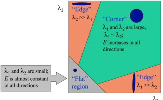
Proposed by Harris and Stephens [Harris and Stephens, 1988] (also known as Harris edge detector), this detector was originally designed to address the problem of finding edges and corners and/or junctions in a tracking system. The Harris detector did this challenge by searching for points x where the second-moment matrix M around the point x has two large eigenvalues.

As seen in Equation 1.1M is calculated as follows; first local image derivatives are computed with Gaussian kernels of scale σD (the differentiation scale) and then the derivatives are averaged in the neighborhood of point x by smoothing with a Gaussian window of scale σI (the integration scale) [Mikolajczyk and Schmid, 2002]. M is a 2 × 2 symmetric matrix, which described the gradient distribution in a local neighborhood of the point x. The matrix M is computed from the first derivatives in a window around x ( i.e. by convolving with a [-2 -1 0 1 2 ] mask), and then weighted by a Gaussian G(x, y, σ_I) kernel with σI = 2 . In other words, matrix M is computed as follows:

M = µ(x, σI, σD) = σ2D× G(σI) ∗    I_x2(x, σD) IxIy(x, σD) IxIy(x, σD) Iy2(x, σD)    (1.1)

where G(.) was the Gaussian operation and I was the image smoothed with the Gaussian function: Ix = ∂ ∂σG(σD) ∗ I(x)&Iy = ∂ ∂σG(σD) ∗ I(y) (1.2) and G(σ) = √ 1 2πσ2exp (− x2+ y2 2σ2 ) (1.3)

Let λ1 and λ2 be the eigenvalues of M, which were proportional to the principal curvatures of the local auto correlation function. If both curvatures were high, it indicates a corner or in other words if:

det(M ) − ktrace2(M ) > t; (1.4)

where det(M ) = λ1λ2 and trace(M ) = λ1 + λ2. By defining the appropriate threshold (t), X could be a corner, edge, or a flat region. Figure 1.3 explains visually how Harris corner detector works. An improved form of Harris detector was proposed later in which the first derivatives were computed more precisely by replacing the the above mask with a Gaussian function with σ = 1.

Förstner Detector

Proposed by Förstner in late 1980s [Förstner and Gülch, 1987] the algorithm aimed at fast detection and precise location of distinct points, such as corners and centers of circular image features − besides lines and area − and finally blobs. Corners ‘beside edges are the basic

(37)

Figure 1.3: Harris corner detector: classification of image points using eigenvalues of M

element for the analysis of polyhedra’ ,. . . “centers of circular features cover small targeted points and holes, disks for rings, which play an important role in one-dimensional image analysis” [Förstner and Gülch, 1987]. The algorithm computed the location of these key-points with a sub-pixel accuracy. To do so, it computed the derivatives on a smoothed image and then calculated the autocorrelation matrix M by summing up the values over a Gaussian mask with the σ = 2. The trace of the autocorrelation matrix was then used to classify region or non-region areas using an automatically chosen threshold. The detector finds the point which is the closest to all tangent lines of a corner in a sub-window of the given image. Hessian Detector

Proposed by Beaudet [Beaudet, 1978] was based on the matrix of the second derivatives or the so-called Hessian Matrix. This 2 × 2 matrix could be obtained from the Taylor expansion of the image intensity function. As the second order derivatives were very sensitive to small variations in neighboring texture and to the noise a Gaussian smoothing step with smoothing parameter σ was done prior to the derivative operation. The Hessian operator could be computed as follows: H = H(x, σ) =    Ixx(x, σ) Ixy(x, σ) Ixy(x, σ) Iyy(x, σ)    (1.5)

where I was the image smoothed with the Gaussian function, and Ixx, Iyyare the second-order Gaussian smoothed image derivatives.

(38)

Figure 1.4: An example of a living room scene and some of the detected Hessian interest points.

3 × 3 neighborhood and applying the non-maximum suppression on this window. In other words the algorithm was looking for the points that makes the Hessain maximal:

det(H) = IxxIyy− Ixy2 (1.6)

Since second-order derivatives were symmetric filters, applying Hessian detector on an image would result in detection of blob-like structure in an image. This results in the maximal to be localized only at ridges and blobs where the size of Gaussian and blob structures matched. Figure1.4shows an example of a scene and its corresponding interest points using the Hessian Detector.

Harris, Hessian and Förstner Detectors has shown to be quite robust to rotation, illumination changes and noise [Schmid et al., 2000]. Since these detectors were computed at fixed scales, i.e. σ, they were not robust to scale changes and were only repeatable to quite small scale variations. In order to detect attributes which were stable to scale changes, scale invariant region detectors such as Laplacian-of-Gaussian, Difference-of-Gaussian, etc. were introduced later.