Intégration de Connaissances aux Modèles Neuronaux pour la Détection de Relations Visuelles Rares

(1)

HAL Id: tel-02917340

https://pastel.archives-ouvertes.fr/tel-02917340

Submitted on 19 Aug 2020

HAL is a multi-disciplinary open access archive for the deposit and dissemination of sci-entific research documents, whether they are pub-lished or not. The documents may come from teaching and research institutions in France or abroad, or from public or private research centers.

L’archive ouverte pluridisciplinaire HAL, est destinée au dépôt et à la diffusion de documents scientifiques de niveau recherche, publiés ou non, émanant des établissements d’enseignement et de recherche français ou étrangers, des laboratoires publics ou privés.

Intégration de Connaissances aux Modèles Neuronaux

pour la Détection de Relations Visuelles Rares

François Plesse

To cite this version:

François Plesse. Intégration de Connaissances aux Modèles Neuronaux pour la Détection de Relations Visuelles Rares. Apprentissage [cs.LG]. Université Paris-Est, 2020. Français. �NNT : 2020PESC1003�. �tel-02917340�

(2)

Ecole Doctorale n°532 : MSTIC - Mathématiques et STIC

Thèse de doctorat

Spécialité Mathématiques

présentée et soutenue publiquement par

François PLESSE

le 27 février 2020

Intégration de Connaissances aux Modèles

Neuronaux pour la Détection de Relations

Visuelles Rares

Directeur de thèse : Françoise PRÊTEUX

Co-encadrement de la thèse :

Bertrand DELEZOIDE

Alexandru GINSCA

Jury

Patrick GALLINARI, Sorbonne Université Président Céline HUDELOT, CentraleSupélec Rapporteur Titus ZAHARIA, Télécom SudParis Rapporteur Gabriela CSURKA, Naver Labs Europe Examinateur Alexandru GINSCA, ATOS Examinateur Bertrand DELEZOIDE, CEA, LIST Examinateur Françoise PRÊTEUX, Ecole des Ponts ParisTech Directeur

(3)

1 Je souhaite en tout premier lieu remercier Françoise Prêteux, Bertrand Delezoide et Alexandru Ginsca qui ont encadré ma thèse durant ces trois années. A Alexandru de m’avoir transmis sa passion pour le Machine Learning et m’avoir apporté son aide et ses idées pour la réalisation des expériences au jour le jour et la rigueur dans la rédaction, à Bertrand qui a guidé mes recherches, m’a partagé sa vision, et relu rigoureusement ce manuscrit. Et à Françoise qui a beaucoup travaillé pour me transmettre sa concision, rigueur et pédagogie dans la présentation de mon travail. Ce fut un véritable plaisir de travailler sur ces sujets avec des encadrants experts de ces domaines à mes côtés.

Je souhaite ensuite remercier Céline Hudelot et Titus Zaharia d’avoir accepté de rapporter sur ce manuscrit, et de m’avoir permis d’améliorer la qualité du manuscrit et de ma soutenance par leurs critiques pertinentes. Un grand merci également à Patrick Gallinari et Gabriela Csurka d’avoir fait partie de mon jury de thèse. Un grand merci également à mes compagnons de thèse Nhi, Othman, Youssef, Umang, Yannick, Eden, Jessica et Dorian, pour toutes nos discussions et nos partages aux cours de ces années communes au CEA. Plus généralement, merci au reste de l’équipe du LASTI, dont Hervé, Adrian, Olivier et Olivier, Romaric, Gaël, Benjamin. Merci à Odile, la secrétaire du LASTI pour son soutien qui m’a permis de m’en sortir pour toutes mes démarches.

Merci à Nikolas, mon colocataire qui m’a soutenu pendant les moments de doutes et pour fêter les moments de réussite. Un grand merci à tous mes autres amis qui m’ont motivé à me lancer dans cette voie : Thomas, Quentin, Cécile, Vivien, Pauline, Alexandre, Martin ainsi que ceux que j’ai malheureusement oublié de mentionner... Enfin, je souhaite remercier les véritables pilliers de cette thése : ma Maman, qui nous a quittés peu avant de pouvoir célébrer ce moment ensemble, mon Papa, mes frères et soeurs et Fabien mon compagnon. Merci pour votre curiosité à chaque fois que vous me demandiez ce que je faisais en ce moment, vos encouragements et votre soutien à toute épreuve pendant ces trois années. Cette thèse vous est dédiée et je vous souhaite bon courage pour sa lecture !

(4)

Intégration de Connaissances aux Modèles

Neuronaux pour la Détection de Relations Visuelles

Rares

François Plesse Résumé

Les données échangées en ligne ont un impact majeur sur les vies de milliards de personnes et il est crucial de pouvoir les analyser automatiquement pour en mesurer et ajuster l’impact. L’analyse de ces données repose sur l’apprentissage de réseaux de neurones profonds, qui obtiennent des résultats à l’état de l’art dans de nombreux domaines. En particulier, nous nous concentrons sur la compréhension des intéractions entre les objets ou personnes vivibles dans des images de la vie quotidienne, nommées relations visuelles.

Pour cette tâche, des réseaux de neurones sont entraînés à minimiser une fonction d’erreur qui quantifie la différence entre les prédictions du modèle et la vérité terrain donnée par des annotateurs.

Nous montrons dans un premier temps, que pour la détection de relation vi-suelles, ces annotations ne couvrent pas l’ensemble des vraies relations et sont, de façon inhérente au problème, incomplètes. Elle ne sont par ailleurs pas suffisantes pour entraîner un modèle à reconnaître les relations visuelles peu habituelles.

Dans un deuxième temps, nous intégrons des connaissances sémantiques à ces réseaux pendant l’apprentissage. Ces connaissances permettent d’obtenir des an-notations qui correspondent davantage aux relations visibles. En caractérisant la proximité sémantique entre relations, le modèle apprend ainsi à détecter une rela-tion peu fréquente à partir d’exemples de relarela-tions plus largement annotées.

Enfin, après avoir montré que ces améliorations ne sont pas suffisantes si le modèle annote les relations sans en distinguer la pertinence, nous combinons des connaissances aux prédictions du réseau de façon à prioriser les relations les plus pertinentes.

Mots Clefs

Vision par Ordinateur, Interprétation Sémantique, Apprentissage Pro-fond, Réseaux de Neurones Convolutifs, Détection de Relations Visuelles, Biais de Sélection, Connaissances Externes, Modélisation Sémantique, Pertinence

(5)

Knowledge Integration into Neural Networks for

the purposes of Rare Visual Relation Detection

François Plesse Short abstract

Data shared throughout the world has a major impact on the lives of billions of people. It is critical to be able to analyse this data automatically in order to measure and alter its impact. This analysis is tackled by training deep neural networks, which have reached competitive results in many domains. In this work, we focus on the understanding of daily life images, in particular on the interactions between objects and people that are visible in images, which we call visual relations.

To complete this task, neural networks are trained in a supervised manner. This involves minimizing an objective function that quantifies how detected relations differ from annotated ones. Performance of these models thus depends on how widely and accurately annotations cover the space of visual relations.

However, existing annotations are not sufficient to train neural networks to detect uncommon relations. Thus we integrate knowledge into neural networks during the training phase. To do this, we model semantic relationships between visual relations. This provides a fuzzy set of relations that more accurately represents visible relations. Using the semantic similarities between relations, the model is able to learn to detect uncommon relations from similar and more common ones. However, the improved training does not always translate to improved detections, because the objective function does not capture the whole relation detection process. Thus during the inference phase, we combine knowledge to model predictions in order to predict more relevant relations, aiming to imitate the behaviour of human observers.

Keywords

Computer Vision, Image Understanding, Deep Learning, Convolutional Neural Networks, Visual Relation Detection, Human Reporting Bias, Ex-ternal Knowledge, Semantic Modelling, Relevance

(6)

Intégration de Connaissances aux Modèles

Neuronaux pour la Détection de Relations Visuelles

Rares

Résumé substantiel en Français

Grâce à de récents progrès qui augmentent considérablement la puissance de calcul, la vitesse de transfert [3] et le stockage de données ainsi que la diminution du prix des processeurs graphiques (GPU) [1], la quantité de données disponible croît très rapidement. 400 heures de vidéos étaient envoyées à YouTube chaque minute en 2015 et 300 millions d’images sont envoyées à Facebook chaque jour [4]. Ces données ont un impact majeur sur la vie de milliards de personnes. Il est par conséquent crucial de les analyser pour être en mesure de comprendre les changements sociétaux qui en résultent, de recommander du contenu pertinent ou d’étudier des marchés potentiels.

Le domaine dédié à l’aggrégation, au traitement et à l’analyse de ces données est appelé pour ces raisons "Big Data". Nous nous intéressons dans cette étude à cette dernière, plus particulièrement à l’analyse d’images. Celle-ci repose, de façon croissante depuis 2012, sur l’utilisation de réseaux de neurones profonds. En effet, Krizhevsky et al. [72] proposèrent un réseau de neurones, appelé AlexNet, atteignant une erreur top-5 de 15.3% sur ImageNet [27], 10.8 points inférieure à l’état de l’art. Cette avancée a suscité de très nombreuses recherches dans le domaine de l’ap-prentissage profond, pour la recommendation de contenus multimedia [21], la prise de décision, le marketing en ligne, la traduction automatique, l’extraction de contenu, etc. De nombreux champs de recherche en explorent l’utilisation pour la décou-verte d’interaction protéine-protéine [138], la génération de vidéos [20], le contrôle d’agents capables de jouer à des jeux de plateau, où les humains restaient jusqu’alors invaincus [129] ou encore de contrôler des voitures autonomes [11]...

Ces dernières avancées apportent par ailleurs une meilleure compréhension du contenu des images, avec la classification d’images [72], la détection d’objets [118,

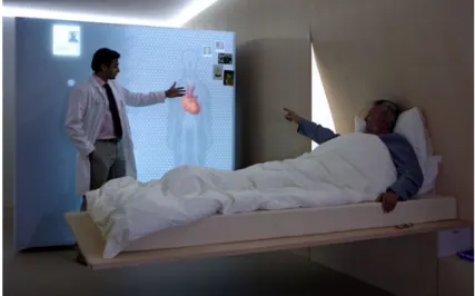
120], la réponse aux questions sur des images [39] et la génération de légendes [157]. Toutefois, les tâches nécessitant des raisonnements haut niveau resistent aux mo-dèles profonds [94]. Des applications telles que l’analyse de contenus provenant de réseaux sociaux ou la conduite autonomes pourraient bénéficier de telles capacités de raisonemment. En effet, la reconnaissance d’actions réalisées par des piétons pour prévoir leur comportement ultérieur nécessite davantage que la détection des objets, comme illustré sur la Figure0.0.1. Ces actions peuvent être déterminées notamment en tenant compte de leurs positions relatives et l’évolution de celles-ci au cours du

(7)

5

Figure 0.0.1 – La prédiction des futures positions des piétons nécessite de les dé-tecter, comprendre leurs directions, leurs intéractions avec ce qui les entoure. temps, ainsi que du contexte de la scène.

Dans cette thèse nous nous concentrons sur la compréhension de ces intérac-tions entre objets ou personnes présents dans une images, et plus généralement, aux relations qui les lient.

Definition 0.0.1 Une relation décrit la manière dont deux personnes ou objets sont connectées ; les effets d’une personne ou d’un objet sur un(e) autre.

Les graphes sont des représentations naturelles de l’ensemble des relations d’une image, les relations étant les arêtes reliant les noeuds representant les objets visibles de l’image. Nous proposons donc d’extraire les relations sous la forme d’un graphe de scène, comme illustré Figure0.0.2.

L’exécution de cette tâche requiert l’extraction automatique de concepts abs-traits à partir d’informations visuelles. Les différences d’angle de vue et de contexte, les possibilités d’occlusion ainsi que les différentes appellations, avec différents ni-veaux d’information, d’un même objet visuel sont la source d’une grande diversité

(8)

6 de représentations d’un même concept. Cela rend l’extraction de ces concepts diffi-cile. L’extraction de relations est d’autant plus ardue que leur représentation dépend non seulement de celles des objets, mais aussi de leurs positions respectives. De plus, certaines relations sont polysémiques et synonynmiques entre elles, ce qui augmente la diversité de leurs représentations visuelles.

Dans cette thèse, nous nous intéressons particulièrement à l’extraction de re-lations par des réseaux de neurones profonds. Ces réseaux sont entraînés par ap-prentissage supervisé. Celui-ci consiste à optimiser une fonction qui caractérise la différence entre les prédictions du réseau et des annotations réalisées par des annota-teurs humains. Les performances de modèles entraînés dépendent ainsi de la qualité de ces annotations, de leur nombre et de la part de l’espace des possibilités qu’elles couvrent et de la précision

Nous montrons que les annotations disponibles pour l’apprentissage de modèles d’extraction de relations ont tendance à être très déséquilibrées. Cela est la consé-quence de plusieurs phénomènes. Tout d’abord, ce problème est de nature combina-toire, le nombre de relations possibles dans chaque image augmentant quadratique-ment par rapport au nombre d’objets présents. Cela rend l’annotation exhaustive d’images très chronophage. Ainsi, les annotateurs doivent choisir des relations parmi l’ensemble des relations possibles. Ces choix ne sont pas complètement aléatoires, car ils dépedent des tailles, distances et positions des objets dans l’image, ainsi que des types d’objets concernés.

Motivés par ces observations, nous étudions l’impact de ce déséquilibre et mon-trons qu’il rend l’apprentissage de certaines classes difficile. Il limite par ailleurs l’évaluation des modèles entraînés, ne rendant pas compte de leur capacité à détec-ter l’ensemble des relations considérées. Pour y remédier, nous proposons de dimi-nuer le besoin en exemples annotés en modélisant les relations sémantiques entre les classes de relations. Cette modélisation permet de caractériser la proximité séman-tique entre relations et profiter des exemples d’une relation plus largement annotée pour apprendre à détecter une relation moins bien dotée. Enfin, la détections de paires d’objets à annoter est un aspect important de la génération du graphe de scène. Nous proposons d’entraîner un classifieur et de pondérer les scores de rela-tions par le résultat de ce classifieur, résultat que nous appelons "pertinence" de la relation. Nous montrons que cela augmente la précision de la détection de relation, augmentant le nombre de vraies relations pour un faible nombre de prédictions.

Pour évaluer les modèles de détection de relations, nous les comparons sur plu-sieurs benchmarks : VRD [89], VG-IMP [158] et deux benchmarks que nous propo-sons, dérivés de Visual Genome [71_{]. Ceux-si sont notés VG-Large, avec plus de}

10 000 classes de relations et VG-RMatters, que nous décrivons plus bas. Nous considérons deux tâches. La première, la classification de graphes de scène (SGCls),

(9)

7 consiste à classifier des régions d’une image et de détecter leurs relations. La seconde, la classification de relations (RelCls) consiste à détecter les relations à partir de régions déjà dotées de classes d’objets. La métrique utilisée est le rappel@k (R@k), où k est un nombre fixé de relations par image.

Biais de sélection de relations

Lors d’une première contribution, nous étudions le déséquilibre des classes de relation dans le benchmark le plus couramment utilisé, Visual Genome [71]. Nous montrons que ce déséquilibre (i) peut-être relié au processus d’annotation (ii) im-pacte l’apprentissage du réseau, entraînant un déséquilibre des relations prédites, très concentrées sur un faible nombre de classes (iii) empêche l’évaluation des mo-dèles de rendre compte de leurs performances dans le cas général.

Nous proposons un réseau de référence, inspiré par plusieurs travaux [41, 166,

170] qui obtient des résultats compétitifs et permet d’évaluer l’impact de ce dés-équilibre. L’extraction de relations est réalisée en plusieurs étapes. Un réseau de neurones convolutif extrait la représentation visuelle de régions correspondant à des détections d’objets et de paires d’objets. Les boîtes englobant les objets sont par ailleurs utilisées pour définir un masque binaire correspondant à la région de l’objet dans l’image, avec la valeur 1 à l’intérieur de la boîte et 0 à l’extérieur. Un nouveau réseau convolutif extrait ensuite la représentation de la configuration spatiale de chaque paire d’objet. Enfin, à partir des représentations visuelles des objets, de la paire d’objet et sa représentation spatiale, quatre branches sont entraînés à prédire des scores correspondant à chaque relation du vocabulaire.

L’apprentissage du réseau, c’est-à-dire la sélection des paramètres, est réalisé en optimisant la fonction ci-dessous par descente de gradient stochastique :

θ = arg max

θ L(θ, D)

= arg max

θ Lo(θ, D) + Lr(θ, D) (1)

où Lo et Lr sont les fonctions d’erreur pour la classification des objets et relations,

définies par l’entropie croisée entre la sortie du réseau et les annotations d’appren-tissage.

Enfin, la génération de graphe de scène est réalisée en sélectionnant les k relations avec le plus grand score, défini par le produit des probabilités de classes d’objets et de relations.

Evalué sur Visual Genome, nous mettons en évidence que le rappel des classes plus rares est très faible, et que cela n’est pas reflété dans le rappel global élevé (88.7%). Nous proposons d’évaluer les modèles sur une métrique supplémentaire :

(10)

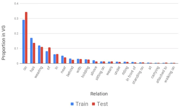
8 le rappel macro par classe, où le rappel est calculé séparément pour chaque classe puis moyenné. Enfin, nous proposons une nouvelle partition du Visual Genome, VG-RMatters, qui augmente la diversité de classes. L’extraction de relations sur cette partition est plus difficile et permet de mieux évaluer les performances des modèles dédiés à cette tâche. La Table0.0.1compare la diversité des relations entre la parti-tion de Visual Genome la plus courante, VG-IMP, et VG-RMatters. La diversité de relations est mesurée par la proportion d’exemples de la classe majoritaire ainsi que l’entropie moyenne des relations par paire de catégories d’objets.

Partition Proportion de la majorité Entropie moyenne VG-IMP [158] 0.62 0.55

VG-RMatters 0.44 0.68

Table 0.0.1 – Proportion d’exemples de la relation majoritaire et entropie dans VG-IMP [158_{] and VG-RMatters pour les 50 paires d’objets les plus fréquentes.}

VG-RMatters a une plus grande diversité de relations.

Modélisation sémantique pour l’apprentissage de

re-lations rares

Dans une deuxième contribution, nous relaxons une hypothèse couramment faite dans l’apprentissage de modèles de détection de relations. Dans de nombreux travaux récents [58,84,154,158,164,166,170], les relations sont supposées mutuellement ex-clusives de façon implicite. Ainsi nous proposons plusieurs méthodes pour apprendre la représentation de relations en considérant leur relations entre elles.

Plus particulièrement, nous entraînons dans un premier temps un réseau dédié à l’extraction de représentations de relations dans un espace métrique, c’est-à-dire un espace doté d’une notion de distance. Contrairement aux travaux qui réalisent l’apprentissage en calculant l’entropie croisée entre deux relations, nous quantifions l’adéquation entre les prédictions du modèle et les données par la distance entre deux paires d’objets correspondant à une même relation. Ainsi nous pouvons relaxer les contraintes imposées au réseau et définir un espace dans lequel les paires d’objets correspondant à des relations similaires sont proches, comme illustré Figure 0.0.3

Cela nous permet par ailleurs de montrer les limites de la représentation apprise, car la différence entre deux relations peut-être due à une différence de configuration spatiales, d’objets, de contexte, etc...

Nous comparons cette méthode à des méthodes utilisant des données textuelles externes. Pour cela, un réseau de neurones est entraîné à respecter une contrainte sémantique. Cette contrainte est définie à partir de représentations de mots, et

(11)

9

(a) Relations similaires (b) Relations spatiales différentes

(c) Actions différentes

Figure 0.0.3 – Représentation t-SNE [141] des relations dans l’espace métrique appris. Les croix correspondent à des relations de l’ensemble de test ; les cercles (mois opaques) représentent des relations stockées pendant l’apprentissage. Notre modèle est capable de regrouper des instances de la même relation, particulièrement les relations bien séparées, telles que "above" et "below ".

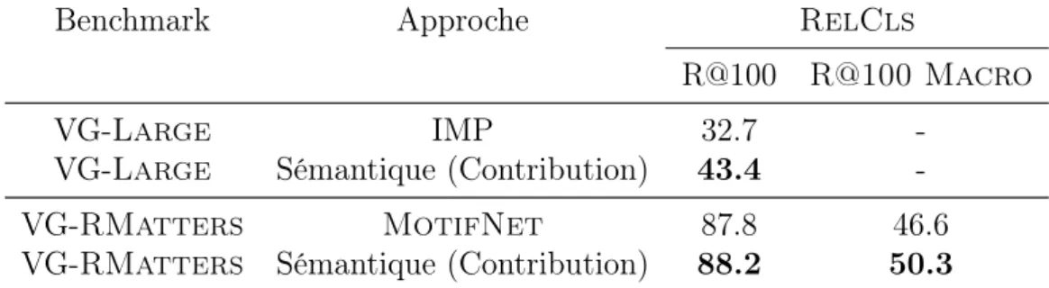
quantifie la proximité entre deux classes de relations. Ainsi le modèle est entraîné à attribuer des probabilités similaires pour des classes apparaissant dans des contextes similaires. Nous montrons la pertinence de cette approche sur un dataset avec un très grand nombre de classes de relations, VG-Large et montrons qu’elle permet d’augmenter le rappel d’une approche de référence de 32%. La Table 0.0.2 résume ces résultats avec la comparaison de notre approche à deux approche à l’état de l’art sur deux benchmarks : VG-Large et VG-RMatters.

Pertinence de relations

Dans une dernière contribution, nous faisons l’observation que de nombreuses paires d’objets sont connectées par des relations non pertinentes, parce qu’elles sont trop courantes (par ex : un arbre a de l’écorce) ou peu intéressantes, car elles concernent des objets petits, distants, etc... Par ailleurs, la faible diversité des rela-tions prédites par les modèles de détection de relation, due au déséquilibre de classes,

(12)

10 Benchmark Approche RelCls

R@100 _{R@100 Macro} VG-Large IMP 32.7

-VG-Large Sémantique (Contribution) 43.4 -VG-RMatters MotifNet 87.8 46.6 VG-RMatters Sémantique (Contribution) 88.2 50.3

Table 0.0.2 – Résultats avec notre approche de modélisation de relations séman-tiques. Notre contribution présente le plus d’intérêt, augmentant signficativement le rappel pour un très grand nombre de classes, tel que VG-Large, et pour les classes rares, comme pour VG-RMatters.

nous motive à concentrer les prédictions sur les relations pertinentes de l’image, pour en augmenter la diversité.

La prédiction de la pertinence d’une relation est difficile, car elle dépend de nombreux facteurs connus (taille, distance, objets ...) et inconnus (liés au processus d’annotation de l’ensemble d’images, liés à l’annotateur ...). Nous proposons donc d’utiliser un classifieur de pertinence, correspondant à la probabilité qu’au moins une relation est annotée. Le score du classifieur est par suite moyenné à un potentiel basé sur des données statistiques mesurées sur l’ensemble d’apprentissage. Ce potentiel permet d’utiliser les relations entre variables dans les prédictions du modèle mais augmente les biais du modèle.

Cette contribution augmente de façon significative le rappel ainsi que le rappel macro de classe, comme le rapporte la Table0.0.3

SgCls RelCls

R@20 R@20 R@20 macro MotifNet [166] 38.0 58.4 19.8

Pertinence (Contribution) 41.0 62.3 23.9

Table 0.0.3 – Résultats avec pertinence de relation sur VG-RMatters. Le rappel est mesuré sur des graphes de scène avec 20 détections de relation.

VG-RMatters est un benchmark difficle, avec des relations variées pour chaque paire d’objets. Pour les images de celui-ci, notre modèle est capable de prédire une plus grande diversité de relations que les modèles à l’état de l’art et d’accroitre le nombre de vraies relations détectées.

(13)

11

Conclusion

La détection de relations visuelles est une étape importante pour comprendre et analyser automatiquement des images. Elle dépend fortement de la qualité de la répresentation des relations. Celles-ci dépendent de la qualité de représentations des objets, ainsi que des dépendances entre représentations visuelles, spatiales et sémantiques. Elles nécessitent donc un grand nombre d’exemples annotés pour les différencier dans des contextes similaires.

Cependant, la nature combinatoire du problème et le biais de sélection de rela-tions rendent le nombre d’annotarela-tions déséquilibré en faveur d’un faible nombre de classes. Cela biaise les modèles appris sur ces données et ne permet pas d’évaluer les performances d’un modèle appliqué à de nouvelles images. Par ailleurs, la faible quantité d’annotation pour un grand nombre de relations ne permet pas d’apprendre à détecter ces relations.

Nous proposons une approche permettant d’intégrer des connaissances externes aux réseaux de neurones profonds, permettant de modéliser les relations entre classes de relations. Le modèle appris est ainsi capable de séparer les relations dans des ré-gions prenant en compte ces similarités et d’utiliser un plus grand nombre d’exemples pour l’apprentissage de chaque classe.

Nous avons par ailleurs montré que la présence de la relation dans l’image n’est pas la seule information à considérer lors de la génération de graphes de scènes. Nous proposons d’intégrer la pertinence de cette relation au processus de génération des graphes de scènes. Ce processus se rapproche ainsi davantage au comportement humain. Par ailleurs, la diversité des relations prédites dans les graphes ainsi généres augmente, concentrant les prédictions sur les relations les plus pertinentes. Cela a pour effet d’augmenter le rappel des classes les plus rares, surpassant les méthodes à l’état de l’art sur plusieurs datasets.

Ces contributions obtiennent des résulats compétitifs, comme le montre la Table

0.0.4. La modélisation de relations sémantiques est la plus pertinente dans le cas

d’un grand nombre de classes, où chaque classe est très similaire à un grand nombre d’autres classes, permettant d’apprendre chaque classe à partir d’un nombre d’exemples beaucoup plus important. Par ailleurs, l’intégration de la pertinence dans la géné-ration de graphes de scènes est l’approche la plus impactante, soulignant le fait que les modèles de l’état de l’art ne capturent pas ou peu cette information.

(14)

12

Benchmark Tâche Etat de l’Art Contribution Résultats Gain Rappel

VRD-set [89] _{RelCls R@20} 81.9 [165]* Sémantique 80.8 -1% VG-IMP [158] _{SGCls R@20} 37.6 [166] Semantique 37.2 -1% VG-IMP [158] RelCls R@20 66.6 [166] Pertinence 66.7 0%

VG-Large RelCls R@50 22.7 [158]** Semantique +_Pertinence 45.2 99% VG-RMatters SGCls R@20 38.0 [166]** Pertinence 41.0 8% VG-RMatters RelCls R@20 58.4 [166]** Pertinence 62.3 7% Rappel Macro

VG-IMP [158] _{RelCls R@100} 37.9 [166] Pertinence 44.4 17% VG-RMatters RelCls R@20 46.6 [166]** Pertinence 52.6 13% Table 0.0.4 – Principaux résultats de la thèse. * sont des réimplémentations et ** sont calculées avec des implémentations mise à disposition par les auteurs. La modélisation de relations sémantiques est la plus pertinente dans le cas d’un grand nombre de classes. L’intégration de la pertinence dans la génération de graphes de scènes est l’approche la plus impactante dans la majorité des cas. Cela souligne le fait que les modèles de l’état de l’art ne capturent pas ou peu cette information.

(15)

Knowledge Integration into Neural Networks for

the purposes of Rare Visual Relation Detection

François Plesse Abstract

Thanks to recent advances in computational power with a steep decrease in the price of Graphical Processing Units and increase in computations per second, data transfer speeds and data storage, more and more data is available. 400 hundred hours of video were uploaded to YouTube every minute in 2015 and 300 million images to Facebook every day. This data has a major impact on the day to day lives of billions of people, and it is critical to understand it in order to comprehend social changes, to recommend relevant content or recognize market opportunities. However, the amount of data makes it impossible for humans to manually extract information out of this content.

This thesis focuses on the automatic analysis of images. Recent advances in object detection have resulted in a sky-rocketting number of applications that rely on understanding the content of an image. However, a thorough comprehension of image content demands a complex grasp of the interactions that may occur in the natural world. The key issue is to describe the visual relations between visible objects. We tackle here the detection of such relations. We call this task Visual Relation Detection (VRD). Many existing methods tackle this task by training deep neural networks with annotated images. This approach is hindered by the gap between visual and semantic representations, whereby visual and spatial represen-tations of one relation have high variability. Indeed these represenrepresen-tations depend on the angle of view of the image, the context, lighting and especially the objects involved in the relation. Additionally, synonymy and polysemy of relations increases this variability.

In light of these issues, we argue that visual information is not sufficient to learn to discriminate between relations. By considering the additional knowledge of relation similarities and focusing on relevant relations, they can be alleviated. Specifically, the major contributions of this work are as follow:

— Human reporting bias in VRD datasets: We show that VRD datasets have exploitable biases that are not apparent due to the used evaluation met-rics. These biases come mostly from a high imbalance in available annotated examples, and a high dependency between objects involved in the relation and the corresponding relation class. We show how this impacts the detec-tions of a competitive baseline and propose a metric as well as a new dataset

(16)

14 to better evaluate the performance of existing methods.

— Overcoming Relation Imbalance with Semantic Modelling: a VRD model is trained so that relations that are similar have similar probabilities. Two methods are proposed: the first method relies on a k Nearest Neighbor approach to train a deep neural network, in order to improve uncommon re-lation classification and take into account the structure of rere-lations. For the second, the standard supervision is augmented with additional constraints from text data, in order to reduce the model bias and increase model gener-alization.

— Relations Relevance: A new scene graph construction method is intro-duced, integrating a learnt relevance criterion. In the absence of annotations for this criterion, two methods are proposed in order to focus on object pairs frequently related in similar contexts. The first relies on self-supervision and the second on high-level dependencies between concepts. The impact of these methods is analyzed showing that the constructed scene graphs contain more uncommon relations while keeping a high overall recall and thus reduces the impact of the reporting bias. Furthermore, we find that this additional factor allows our model to predict relations on fewer and more relevant object pairs.

(17)

4.3.3 Data Augmentation with synonymy-compatible distributions . 126 4.3.4 Rule distillation . . . 127 4.3.5 Experiments . . . 131 4.3.6 Discussion . . . 140 4.4 Conclusion . . . 140 5 Relation Relevance 142 5.1 Context . . . 143 5.1.1 Motivation . . . 143 5.1.2 Related Work . . . 145 5.1.3 Formulation . . . 146

5.2 TopicNet: Learning Relation Representations with Attention to Topic 146 5.2.1 Motivation . . . 146

5.2.2 Related Work . . . 147

5.2.3 Describing images with latent topics . . . 147

5.2.4 Visual Relation Detection with Attention to topic . . . 150

5.2.5 Experiments . . . 152

5.2.6 Discussion . . . 155

5.2.7 Conclusion . . . 158

5.3 Focused VRD with Prior Potentials . . . 160

5.3.1 Motivation . . . 160

5.3.2 Relevance Estimation with Prior Potentials . . . 160

5.3.3 Experiments . . . 163

5.3.4 Discussion . . . 170

5.4 Conclusion . . . 170

6 Conclusion and perspectives 171 6.1 Main Contributions and Associated Perspectives . . . 172

6.1.1 Human Reporting Bias in Relation Annotations . . . 173

6.1.2 Overcoming Relation Imbalance with Semantic Modelling . . . 174

(20)

Contents 18

6.2 Future Directions . . . 176

Appendices 177

A Human Reporting Bias and Class Output Probabilities 178

(21)

List of Figures

0.0.1 La prédiction des futures positions des piétons nécessite de les

détecter, comprendre leurs directions, leurs intéractions avec ce

qui les entoure. . . 5

0.0.2 Image extraite du Visual Genome [71] et le graphe de scène associé. 5 0.0.3 t-SNE embedding of relation representations learnt by ProtoNN . 9 1.2.1 Types of concepts. . . 27

1.2.2 Two images from Visual Genome [71] and their respective anno-tated scene graphs. . . 28

1.2.3 Relation "on the left of " for different viewpoints. . . 29

1.2.4 Relation "fish in" for different object pairs . . . 29

1.2.5 Examples of polysemy and synonymy . . . 29

1.3.1 Multiple relations for one object pair . . . 31

2.1.1 Schema of Neural Network with two layers . . . 36

2.6.1 Common VRD pipeline. . . 60

2.6.2 Visual relations from Visual Genome . . . 61

2.6.3 Sit on Visual Genome . . . 62

2.6.4 Relation distribution in Visual Genome . . . 65

2.7.1 Images from Stanford 40 actions dataset . . . 69

2.7.2 Images from the VRD-set dataset . . . 69

2.7.3 Images from Visual Genome . . . 70

2.7.4 Graph constraints on Scene Graphs . . . 73

3.1.1 Hundreds of true relations per image . . . 80

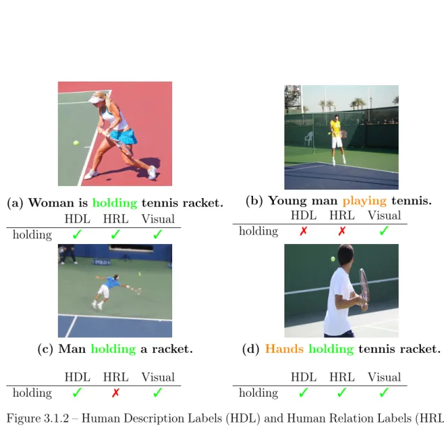
3.1.2 Reporting Bias in Visual Genome . . . 83

3.2.1 Proportion of examples in Visual Genome with the VG-IMP split 84 3.2.2 Relation distribution by pair of object categories . . . 86

3.3.1 Visual Relation Detection Baseline . . . 89

3.3.2 Evolution of cross-entropy loss over 9 epochs . . . 91

3.3.3 Performance at each epoch on the Train set . . . 92

3.3.4 Performance at each epoch on the Validation set. . . 93

3.3.5 Performance at each epoch on the Test set . . . 93

(22)

List of Figures 20

3.3.6 Histogram of Probability that any relation is true . . . 94

3.3.7 Distribution of baseline output probabilities for object pairs

an-notated with relations. . . 96

3.3.8 Confusion Matrix of our Baseline . . . 97

3.3.9 Output example 1 . . . 99

3.3.10 Output examples 2 and 3 . . . 100

3.4.1 Limitations in generation of dataset with uncommon relations . . 103

3.4.2 Comparison of distributions of relation classes in test sets . . . . 104

3.4.3 Comparison of distributions of relation classes for each object

category . . . 105

3.4.4 _{Probability of guessing the correct relation in VG-RMatters} . . 107

4.1.1 Confusion Matrix of our Baseline . . . 109

4.1.2 Several true relations describe the elected pair at different

seman-tic levels . . . 110

4.2.1 Processing pipeline of Learning Relation Prototypes . . . 113

4.2.2 Word cloud of a cluster with relations (person, clothing) pairs. . . 115

4.2.3 Word cloud of a cluster with relations entailing close positions . . 115

4.2.4 Word clouds a cluster with (animal/person, flat surface) pairs. . . 115

4.2.5 t-SNE embedding of relation representations learnt by ProtoNN . 118

4.2.6 t-SNE [141] embedding of relation representations learnt by

Pro-toNN for relation classes of VRD-set. Crosses correspond to test relations and circles (less opaque) to prototypes stored during the training phase. Our model learns to cluster semantically close

ex-amples, such as (person, relation, clothes) triplets.. . . 119

4.2.7 Examples of retrieved nearest neighbors for four test examples . . 120

4.3.1 Semantic Distillation . . . 130

4.3.2 Relation recall by the number of train examples in VG . . . 135

4.3.3 Relation recall for each relation class . . . 137

4.3.4 Confusion matrix of SK (top) and difference with the Baseline

confusion matrix (bottom). . . 138

4.3.5 Similarity matrix between relations in VG . . . 139

5.1.1 _{Confusion matrix of our Baseline on VG-RMatters} . . . 144

5.1.2 Examples from Visual Genome. The relation (tree, has, bark) is

annotated in leftmost image but not in the rightmost image. . . . 144

5.2.1 Top associated objects and images of two topics . . . 149

5.2.2 _{TopicNet framework} . . . 151

(23)

List of Figures 21

5.2.4 Top k recall for topic classification among 90 topics. Due to the

redundancy between topics, we focus on recall after several pre-dictions. At 6 predictions, the recall is at 91%. We conclude that

the network learns to classify the image topic. . . 157

5.2.5 _{Extracted scene graphs for MotifNet and TopicNet} . . . 159

5.3.1 _{FocusedVRD framework} . . . 161

5.3.2 _{Recall per relation class for MotifNet and FocusedVRD on}

VG-RMatters . . . 165

5.3.3 Image example from VG and associated scene graph . . . 168

5.3.4 Estimated Probabilities that any relation is annotated from

Rel-evance Classifier, Prior Potential and the combination. . . 169

A.0.1 Classification scores for each class . . . 179

B.0.1 Output example with and without relevance . . . 183

B.0.2 Output example with and without relevance . . . 184

(24)

List of Tables

0.0.1 Entropy and proportion of the majority relation for in VG-IMP

and VG-RMatters . . . 8

0.0.2 Summarized results with Semantic Modelling . . . 10

0.0.3 Summarized results with Relevance . . . 10

0.0.4 Résultats . . . 12

2.1.1 Object Detection Results on MS-COCO [86] . . . 39

2.2.1 Deep metric learning . . . 43

2.2.2 Few-shot learning on Omniglot . . . 43

2.3.1 Performance of Transfer Learning on Pascal VOC 2012 [32]. . . . 46

2.3.2 Multimodal learning . . . 47

2.3.3 Knowledge Distillation . . . 48

2.3.4 Hierarchical Semantic Modelling. . . 49

2.4.1 Knowledge distillation . . . 53

2.4.2 Self-supervised learning . . . 55

2.4.3 Attention . . . 56

2.5.1 Resampling . . . 58

2.6.1 Visual Relation Detection methods . . . 68

2.7.1 Characteristics of existing splits of Visual Genome. . . 70

2.7.2 State of the Art on VRD-set . . . 74

2.7.3 State of the Art on Visual Genome with constraints . . . 74

2.7.4 State of the Art on Visual Genome without constraints . . . 74

2.8.1 Visual Relation Detection methods . . . 76

3.3.1 Results Distribution with Bootstrapping . . . 94

3.3.2 Results of our baseline on VG . . . 101

3.4.1 Entropy and proportion of the majority relation in VG-IMP and

VG-RMatters . . . 103

3.4.2 _{Performance on VG-RMatters.} . . . 106

4.2.1 _{Results of ProtoNN on VRD-set} . . . 123

4.2.2 _{Results of ProtoNN on VG-IMP} . . . 124

(25)

List of Tables 23

4.3.1 Results of Explicit and Implicit models of synonyms on VRD-set

and VG-IMP . . . 131

4.3.2 _{Results of Semantic and Internal Distillations on VG-Large}. . . 132

4.3.3 _{Results of Semantic and Internal Distillations on ImMacro on}

VRD-set . . . 133

4.3.4 Results with Semantic Distillation on VG-IMP. . . 134

4.3.5 _{Results with Semantic Distillation on VG-RMatters} . . . 134

5.2.1 _{Results with 4 streams on VG-RMatters} . . . 153

5.2.2 _{Results of TopicNet with 1 and 4 streams} . . . 154

5.3.1 _{Recall of FocusedVRD on VG-IMP} . . . 164

5.3.2 _{Ablation study on VG-RMatters} . . . 166

(26)

Chapter 1 Introduction

(27)

Motivation 25

1.1 Motivation

Thanks to recent advances in computational power, with a steep decrease in the price of Graphical Processing Units (GPUs) [1], in data transfer speeds [3] and data storage, more and more data is available. For instance, four hundred hours of video were uploaded to YouTube every minute in 2015 and 300 million images to Facebook every day [4]. This data has a major impact on the day to day lives of billions of people, and it is critical to understand it in order to comprehend social changes, to recommend relevant content [21] or recognize market opportunities.

Thus deep learning models have been adopted in many different sectors, such as recommendations for multimedia services or electronic stores. They are also increasingly used for decision making, online marketing, automatic translation, con-tent extraction. Many research fields explore their use for protein-protein interaction [138], video generation [20], agents able to play games [129], to control self-driving cars [11] and so on.

However, these models present several noticeable flaws. Indeed, deep learning models are much less efficient at generalization and learning complex rules than humans, as shown in [76, 77], requiring hundreds of labeled examples to learn new concepts. In [94], Marcus shows that models trained by reinforcement learning have a very shallow understanding of the space with which the agent interacts. After being trained for several hundred hours on a single game, their performance can be thoroughly undermined with small perturbations. Furthermore, when it comes to text understanding, recurrent neural networks do not adapt well to differences in test and training test that require compositional skills. This is in part due to the representation of sentences as word sequences whereas language is intrinsically hierarchically structured, as argued by linguist Noam Chomsky [19].

These limitations are symptoms of the fact that deep learning models are very good at finding correlations between variables, whether these variables are features of images, text documents or sound... However, these correlations are not always always related causally, i.e. one variable is not the cause of the other and vice versa. For example, Ribeiro et al. [121] show evidence that, when trained on a small dataset with pictures of wolves and huskies, the wolf classifier only learns to detect snow. Features associated with snow textures are the most statistically distinguishing feature but this relationship is not causal.

Furthermore, recent studies [31, 45] suggest that some non-causal relationships learnt by deep learning models arise from a phenomenon whereby models latch on high-frequency information. They show that a model is able to recognize images

(28)

Basic Concepts and Issues related to Visual Relation Detection 26 passed through a high-pass filter, recognizing images that are nearly invisible to humans. This makes it sensitive to additive high-frequency noise, which explains why adversarial examples are so efficient at fooling deep neural networks.

The latter limitations can be tackled by adversarial training, while the former, i.e. learning spurious correlations between low-frequency features, mainly have im-plications in specific settings. Such settings tend to have small datasets or strongly differing training and testing distributions (e.g. if all wolves in train are in snowy contexts but not in test). With the advent of large datasets such as ImageNet [27] and transfer learning techniques [106], the drawbacks of small datasets can be mitigated. Many solutions have been proposed accordingly, on the one hand by integrating external knowledge, in the form of class attributes for zero-shot learn-ing [78, 108, 155] and on the other hand by bringing together symbolic and neural modelling. The latter works involve discrete operations with neural models [101], use a combination of reinforcement learning that learns to translate sentences into symbolic programs and supervised learning to learn scene representations [92] for Visual Question Answering.

Thus, despite large strides in image understanding with tasks such as image classification and object detection, neural models perform poorly at tasks that do not only require recognition but also higher level reasoning [94]. Applications such as autonomous driving and social media analysis for purposes of epidemiology or market analysis could benefit such reasoning. To recognize the action in which pedestrians are engaged in, or how many people are smoking in a picture, one needs not only detect all visible objects but also how they interact. These interactions depend on the relative positions of objects and people and their respective parts, as well as the context around them.

1.2 Basic Concepts and Issues related to Visual

Re-lation Detection

Let us introduce several basic concepts on which this work is based.

Definition 1.2.1 A concept is a general and abstract idea of a concrete or abstract object made by a human mind, allowing it to connect to it perceptions and organize knowledge.

This definition adapted from Larousse Dictionary underlines the important con-nection between perception and knowledge that are necessary to understand the

(29)

Basic Concepts and Issues related to Visual Relation Detection 27 world. Concepts can be partitioned in several categories: objects, actions, scenes and so on, as shown in Figure1.2.1.

Figure 1.2.1 – Several types of concepts may be extracted from one image. Here: objects: man, frisbee, actions: throwing frisbee, scene: outdoor sports.

The detection of a type of high-level concepts which describes interactions, rel-ative spatial configurations and possession, which we call relations, is the object of this dissertation.

Definition 1.2.2 A relation describes the way in which two people or things are connected; the effect of a person/thing on another.

Relations are the description of how objects interact, thus graphs are natural representations of these high-level concepts. Hence, we propose to extract such relations from still images in the form of scene graphs. Scene graphs are graphs comprised of object nodes, representing objects visible in the image and relation-ship edges, representing true relationrelation-ships between the objects of the image. Two examples of such graphs are represented in Figure 1.2.2.

Tackling this task requires the automatic extraction of concepts from visual information. As mentioned in [6], this raises the problem of the semantic gap, which characterizes the differences between a concept and its representations in different modalities. Visual representations of a concept have high variability due to multiple factors: membership to different sub-concepts, angle of view, occlusion, context, lighting and so on. This is especially true when it comes to the relations between objects because their representations vary depending on perspective and especially depend on the involved objects.

(30)

Basic Concepts and Issues related to Visual Relation Detection 28

Figure 1.2.2 – Two images from Visual Genome [71] and their respective annotated scene graphs.

Figures 1.2.3 and 1.2.4 show how this gap manifests for spatial relations (e.g. on the left of ) (resp. actions (e.g. fish in)) with different viewpoints (resp. differ-ent object pairs). In these examples the underlying relation concept remains the same while both low level visual representation and spatial configurations are very different.

This semantic gap manifests in a second way as shown in Figure1.2.5due to the polysemy of relations.

Definition 1.2.3 Polysemy is the phenomenon whereby a single word form is as-sociated with two or several related senses.

Polysemy of relations increases this gap by increasing the variability of the visual representation of relations. For example, with relation "in", the shape of the object one is "in" will imply very different spatial configurations as illustrated in Figure

(31)

Basic Concepts and Issues related to Visual Relation Detection 29

(a) parking meter on the left of skier (b) boy in red on the left of boy in black

Figure 1.2.3 – Relation "on the left of " for different viewpoints, i.e. where the photographer is behind the object pair (a) or in front of the object pair (b). The spatial configuration of the relation depends on the of position of the photographer relative to the objects.

(a) person fishing in sea (b) bear fishing in river

Figure 1.2.4 – Relation "fish in" for different object pairs. The visual representation of one relation is highly influenced by that of the involved objects.

(a) dog in car (b) dog in shirt (c) woman in hat (d) woman wearing hat

Figure 1.2.5 – On the one hand, a polysemous relation can have several meanings and thus have a high intra-variability, as in (a), (b) and (c). On the other hand, in several contexts, different relations can have the same meaning and have similar visual representations, as in (c) and (d): they are synonymous.

Definition 1.2.4 Synonymy is the phenomenon whereby two different words are associated with the same sense.

Synonymy does not participate in the semantic gap but increases the confusion between relations and directly ties into the problem of polysemy as relations can be synonymous in some contexts and have different meanings in others. For example

(32)

Problem statement 30 the relation "in" in dog in shirt is synonymous to "wear ". However with the pair (dog, car), this synonymy does not hold anymore.

1.3 Problem statement

Having defined these concepts, we formally define the task of Visual Relation Detection. We consider the problem of scene graph labelling, i.e. of defining a function that takes as input a real valued image and outputs a scene graph with labeled nodes and edges. Let f be a graph labelling function

f : RhI×wI _{→ Seq({0, 1}}nC_{) × Seq({0, 1}}nR₎ _(1.1) where Seq(X) denotes the spaces of finite sequences in X and hI and wI are the

dimensions of input images. The number of object and relations classes are referred to as nC and nR, respectively.

Given an image I,

f : I 7→ ({v1, . . . , vn}, {e1,1, . . . , en,n−1}) (1.2)

is a labeling of I and for all i ∈ [1 . . . n] and k ∈ [1 . . . nC]

vi,k =

  

1 if ck is a label for object i

0 otherwise.

(1.3) and for all h, t ∈ [1 . . . n], h 6= t, k ∈ [1 . . . nR]

eh→t,k =

  

1 if rk is a label for edge (h, t)

0 otherwise.

(1.4) This allows the mapping to assign multiple labels to one node or edge leading to a multi-label classification. We make this choice because several relations may be true for one pair of objects, especially spatial relations and actions, or different compatible actions as in Figure1.3.1.

Furthermore, for each object pair (h, t), one relation may be true without being annotated by a human. Thus we propose to distinguish two tasks, with different challenges, which we explore in depth in this work:

1. Relevance Classification is the task consisting in predicting whether at least one relation is annotated, i.e. there exists k ∈ [1 . . . nR] such that

(33)

Report Outline and Contributions 31 2. Relation Classification consists in predicting what relation is true, given

that at least one is annotated

Figure 1.3.1 – Image example from Visual Genome [71]. Several relations are true between the selected objects: (person, right of, frisbee), (person, holding, frisbee), (person, throwing, frisbee), (person, with, frisbee)...

1.4 Report Outline and Contributions

The obstacles presented in Section 1.2 and Chapter 3 are the main motivation for the contributions of this work, summarized as follows.

— In a first Chapter, we study how several limitations of Deep Neural Net-works impact these netNet-works and how they pertain to the issues related to VRD. Then we show how they can be tackled and how they can be applied in the context of VRD.

— In a second Chapter, we show some limitations to existing VRD methods. We show that, due to the human reporting bias, the evaluation of the loss function does not accurately represent the true relation distribution and thus models do not generalize to new images. Furthermore, we show that the loss function does not correlate with performance on the target metric. Finally, having shown that evaluation of existing models on imbalanced datasets does not completely capture their performance, we propose a new metric and a new split of the most studied VRD dataset, in order to highlight these limitations. The definition of this split has been submitted to WACV 2020.

— The foremost limitation is the poor performance of the detection of rarer relations, which we tackle in a third Chapter by modelling semantic re-lationships between relation classes. We integrate semantic knowledge into the network during the training phase in order to improve the accuracy of the relation distribution estimation. We propose two methods for modelling semantic relations, which respectively bring a 13% and 33% relative increase

(34)

Report Outline and Contributions 32 in recall averaged over classes (resp. images). These results have been pre-sented in two separate publications [113,114] and in an extended publication submitted to MTAP 2019.

— Finally, in a fourth Chapter, we show that the scene graph generation pro-cess is critical to the performance of our VRD model. Knowledge is here combined to the model predictions during inference, in order to tackle prob-lems that are not captured by the training objective. Introducing a new relevance classifier, we can significantly increase the recall of relations, espe-cially that of rarer relations, increasing the recall averaged over all classes by 13%. This contribution was introduced in our publication [113] and further proof of its impact is shown in our work submitted to WACV 2020.

(35)

Chapter 2 State of the Art

(36)

Neural Networks 34 This chapter consists of a survey of the Visual Relation Detection (VRD) field. However, this is a very young field, therefore many existing methods that have been proposed in related fields such as object detection, image classification, few-shot learning, have not been applied to VRD. As all VRD competitive methods make use of Deep Neural Networks. Before diving into this task, we give a broader introduction of the training process of Deep Neural Networks and present some of these methods.

2.1 Neural Networks

Our goal is to extract from a still image a scene graph. To achieve this, we aim to define an image labeling function that takes as input any image and outputs this scene graph. This function can then be evaluated by several measures, such as the fraction of true relations in the output graph, the fractions of true relations in the image that are present in the graph and so on.

This task is part of a greater set of problems which can be described as finding a mapping f : X → Y between an input vector space X of dimension din and an

output space Y . This mapping should satisfy a set of constraints. For example, in the case of VRD, the input space X is the set of possible images, Y the set of possible scene graphs.

Constraints on f would be that for each I in X and (o1, r, o2) in f (I), objects o1

and o2 are present in I and the relationship triplet (o1, r, o2) is true. In this work, we

consider relations between detected objects. Thus a relation between two objects is true if and only if

1. both objects are correctly classified

2. the relation between the objects holds true

2.1.1 Definition

When considering tasks such as image or text understanding, input and output spaces have several thousand dimensions. For images, this is due to the number of pixels and for texts, to the number of possible word combinations. In recent years, both the quantity of available data and computational power has increased very rapidly, making supervised learning approaches competitive in the task of deriving such mappings. These methods are based on training parametric models with an-notated data so that the models are able to reliably predict labels for unaan-notated data.

(37)

Neural Networks 35 Supervised Learning Let D, a dataset comprised of input pairs {(x1, y1), . . . , (xn, yn)}

where for each i ∈ [1 . . . n], (xi, yi) ∼ p is drawn independently and identically

dis-tributed with a distribution p : (X, Y ) → R+.

Supervised learning is a subset of Machine Learning algorithms. The aim of these algorithms is to find a mapping over a specified space of mappings F that best fits the training data. The space F is defined as {fθ| θ ∈ Rd}: a set of parametric

functions, parameterized by a vector of parameters θ.

For this, an objective function φ is defined to quantify the fit between a given sample (xi, yi) ∈ D and the output ˜yi = f∗(xi). Thus f∗ is defined as

f∗ = arg min

f ∈FE(x,y)∼p[φ(f (x), y)] (2.1)

The search of this mapping is called training. As mentioned in [53], this makes train-ing models different from optimization problems, where the performance measure is directly optimized. In contrast, neural networks are evaluated on another metric M . However, its optimization is usually not tractable, which is why a different object function is optimized, in the hope that it improves M .

In Equation2.1, the mapping is defined as the function that minimizes the risk. In practice, this expectation is usually not available so the experimental risk is optimized instead: f∗ = arg min f ∈F 1 n X (x,y)∈D φ(f (x), y) (2.2) While the standard error of this estimation is equal to √σ

n where σ is the standard

deviation of {φ(f (x), y)}(x,y)∈D and decreases with the number of examples n, the

computation of the gradient for equation 2.2 is linear with respect to n. in D. For very large datasets, this becomes intractable and thus motivates the use of Stochastic Gradient Descent [67, 122], where the gradient of the function is estimated using a sample of the training set, called a minibatch.

Finally, the training process differs from the optimization process because of early stopping. Since the objective function is different from the target metric, an additional criterion is used to select a stopping point for the optimization process, typically evaluating the target metric M on a validation set defined beforehand.

As most competitive methods that tackle computer vision tasks, VRD included, are based on Neural Networks, we study in this section this class of mappings. They do not require to manually define a representation of the input data but instead directly use its raw representation. can be defined as the composition of a number of parametric functions such as affine functions and activation functions as illustrated on Figure2.1.1. From this, we can define:

(38)

Neural Networks 36 Inputs Parametric Function Parametric Function Activation Function Activation Function Outputs

Figure 2.1.1 – Schema of Neural Network with two layers, taking a 6-dimensional input and outputting a two-dimensional vector. Each layer is defined as the compo-sition of a parametric and activation function. Here both parametric functions are affine functions summing a weighted sum of inputs and a bias. They are followed by one activation function.

A Neural Network is a parametric mapping f defined as the composition of parametric functions and activation functions optimized to minimize an experimen-tal risk on a set of inputs.

2.1.2 Classifiers

We specifically focus on the task of classifing inputs (e.g. images) into a set of classes Y = {1, . . . , nc}. Thus we consider classifiers, i.e. a class of mappings

from a vector space X to a discrete finite space. To use Deep Neural Networks as classifiers, they are usually defined such that an intermediate representation of the input, noted x0, is extracted. Then the last layer of the neural network is set as the affine function:

x0 → ˜y = W · x0+ b (2.3) where W ∈ Rd0×nc _{and d}0 _{is the dimension of x}0_{. The conditional probability of class} i is then computed with the softmax function

q(y = i|θ, x) = _P_nexp ˜_c yi

k=1exp ˜yk

(39)

Neural Networks 37 where θ is the set of parameters. The model parameters are then defined as the parameters maximizing the log likelihood function:

θ∗ = arg max X (x,y)∈D log q(y|θ, x) (2.5) = arg max X (x,y)∈D nc X j=1

p(y = j|x) log q(y = j|θ, x) (2.6) = arg max −H(p, q) (2.7) = arg min H(p, q) (2.8) where H is the cross-entropy function.

2.1.3 Convolutional Neural Networks

Having defined how the output distribution is extracted, we now study how the intermediate representation is extracted. In this work, where the input is an im-age, this representation is extracted by convolutional layers. Indeed, Convolutional Neural Networks have reached competitive results when processing images, due to several properties which we explain after describing how these layers process inputs. Convolutional Neural Networks (CNNs) are a class of neural networks where the parametric function are kernels which are convoluted over their input. Let f a convolution layer. f (I)(i, j) =X m X n I(i − m, i − n)K(m, n) (2.9) where K is a two-dimensional kernel.

As mentioned in [53], the motivation behind these convolutional layers is inter-action sparsity, parameter sharing and representation equivariance to trans-lation. The first refers to the smaller size of the kernel when compared to the input, decreasing the number of parameters and the number of operations. The second refers to the sharing of parameters between different image positions. Contrary to feed-forward layers, the output of a single channel is parameterized by a single kernel for all image locations. Finally, equivariance to translation means that if the input is translated by a given amount, then the output is translated by the same amount. Thus these networks are efficient with respect to the number of used parameters and are well adapted to large grid-structured inputs which is why they are very widely-used for image processing tasks.

(40)

Neural Networks 38

2.1.4 Object detection

Object Detection is the first step towards VRD, as it is required to define the nodes in the image scene graph. An object detector is a mapping from an image input space X into the set of finite object sequences Y = Seq(R4_{× C), where for}

each y = (b, c) ∈ Y , b corresponds to the coordinates of the object bounding box and c is in C = {0, 1, . . . , nc}, a finite set of object classes.

Finding a mapping that minimizes a given objective function is a task that can not be solved by the same architectures as image classifiers as the number of outputs changes depending on the input. A naive approach would rely on first extracting a set of regions of interest then processing each part of the image bounded by a box and classify the presence of an object. However, this process is inefficient in computation time as well as memory as the number of necessary proposals to obtain a high detection score would be too high.

Regions with CNN features (R-CNN) To bypass this problem, Girshick et al. [48] proposed R-CNN, a model taking as input a set of 2,000 region proposals extracted with Selective Search [140], which extracts a representation of each region by passing them through a pre-trained CNN, and taking the output of a dense layer, then classifying each one using binary SVMs. Furthermore, a linear regression is trained to predict more accurate bounding box coordinates. The main drawback of this method are the processing of a high number of regions of interest by a neural network, resulting in a 47s average processing time per image.

Fast R-CNN This drawback is addressed by Girshick et al. [47] with the Fast R-CNN model. It is able to extract a representation of each region proposal by processing the image once using ROI-pooling with the same region proposals as in [48]. ROI-pooling consists of extracting a fixed-sized grid representation of each region proposal, by pooling the maximum value at each grid location. Since the ROI-Pooling operation is differentiable, the network can be trained from end-to-end, after a pre-training, which allows Fast R-CNN to outperform R-CNN from 62.4 to 65.7 mean Average Precision (mAP) on VOC 2012 [32] while decreasing the processing time from 47s to 2.3s per image at test time.

Faster R-CNN The last method has two drawbacks: the region proposal method is still separated from the object detection model, which makes errors at the proposal level impossible to correct. Furthermore, most of the processing time comes from the high number of region proposals of Fast R-CNN (2,000). Instead of using Selective Search, Ren et al. [120] define a sub-network called RPN (Region Proposal Network). A grid is defined over the extracted feature map of the image with a set of 9 anchors

(41)

Neural Networks 39 at each point of the grid. After removing duplicate detections with Non Maximum Suppression (NMS), the number of region proposals is decreased to 300. They then define an error function to evalutate the quality of each object region detection used to update the model parameters. For each selected anchor, an objectness score and bounding box coordinates are output by a softmax classifier and the same regressor as in Fast R-CNN. The object detection is then used witht the same network as in Fast R-CNN, sharing convolutional layers with the RPN. With their proposed training procedure, the mAP increases from 65.7% to 67.0% without additional training data, and 75.9% with pre-training on MS COCO and Pascal VOC 07 [32], with a decreased processing time of 0.2s per image [120].

You Only Look Once You Only Look Once (YOLO) [119] changes the paradigm of object detection by removing the need of region proposals. Instead, the image is divided into a grid of fixed dimensions and the network predicts two bounding boxes at each grid location with a confidence score and class probabilities at this point, independently from the bounding box and in only one forward pass. Thus the whole image impacts the detection at each point and any predicted bounding box will have the most probable class of the corresponding grid point. This also makes the object detection much faster. Their final version [118] decreases the processing time to 0.025s per image with a mAP of 78.6%, higher than Faster R-CNN.

Method AP Faster R-CNN [120] 34.9 Yolov3 [118] 33.0

Table 2.1.1 – Object Detection Results on MS-COCO [86]

Table 2.1.1shows results for object detection on MS-COCO [86]. Faster R-CNN is slower than YOLO but outperforms it on the task of object detection. We focus on Faster R-CNN because they have been shown to provide representations of images that can be used in diverse tasks (see Section2.3.1, at the cost of processing speed.

2.1.5 Caption generation

The task of caption generation, which consists of finding a mapping from an image space to the space of finite sequences of words has garnered interest with applications from image retrieval [160] to automatic image description for visually impaired people [90]. It is similar to Visual Relation Detection, as both tasks consist in extracting higher order descriptions than detecting objects. The outputs of Cap-tion GeneraCap-tion models however are unstructured, contrary to those of VRD models.

(42)

Neural Networks 40 This makes captions more flexible but also less readily usable for downstream tasks, such as image retrieval.

Competitive models are comprised of two successive neural networks. One is a CNN acting as image encoder, representing the image in a much lower dimensional space. The second is a recurrent neural network decoding the encoded image into a set of sentences. Vinyals et al. [145] propose to use a CNN pre-trained as an image classifier on ImageNet [49] and an LSTM (Long Short-Term Memory) [60] network taking as context the image encoding and the previously predicted words. The network is then trained to maximize the log likelihood of the correct word. This method is extended in [159] with an attention mechanism (see Section 2.4.5) that attributes higher weights to parts of the image for the prediction of each word.