HAL Id: hal-01241978
https://hal.inria.fr/hal-01241978
Submitted on 18 Dec 2015
HAL is a multi-disciplinary open access
archive for the deposit and dissemination of
sci-entific research documents, whether they are
pub-lished or not. The documents may come from
teaching and research institutions in France or
abroad, or from public or private research centers.
L’archive ouverte pluridisciplinaire HAL, est
destinée au dépôt et à la diffusion de documents
scientifiques de niveau recherche, publiés ou non,
émanant des établissements d’enseignement et de
recherche français ou étrangers, des laboratoires
publics ou privés.
Scale-Adaptive Forest Training via an Efficient Feature
Sampling Scheme
Loic Peter, Olivier Pauly, Pierre Chatelain, Diana Mateus, Nassir Navab
To cite this version:
Loic Peter, Olivier Pauly, Pierre Chatelain, Diana Mateus, Nassir Navab. Scale-Adaptive Forest
Training via an Efficient Feature Sampling Scheme. Medical Image Computing and Computer-Assisted
Intervention, MICCAI 2015, Oct 2015, Munich, Germany. �hal-01241978�
Scale-Adaptive Forest Training via an Efficient
Feature Sampling Scheme
?Lo¨ıc Petera, Olivier Paulya,b,??, Pierre Chatelaina,c, Diana Mateusa,b,
Nassir Navaba,d
a
Computer Aided Medical Procedures, Technische Universit¨at M¨unchen, Germany bInstitute of Computational Biology, Helmholtz Zentrum M¨unchen, Germany
c
Universit´e de Rennes 1, IRISA, France d
Computer Aided Medical Procedures, Johns Hopkins University, USA
Abstract. In the context of forest-based segmentation of medical data, modeling the visual appearance around a voxel requires the choice of the scale at which contextual information is extracted, which is of crucial im-portance for the final segmentation performance. Building on Haar-like visual features, we introduce a simple yet effective modification of the for-est training which automatically infers the most informative scale at each stage of the procedure. Instead of the standard uniform sampling during node split optimization, our approach draws candidate features sequen-tially in a fine-to-coarse fashion. While being very easy to implement, this alternative is free of additional parameters, has the same computa-tional cost as a standard training and shows consistent improvements on three medical segmentation datasets with very different properties.
1
Introduction
Among the existing statistical learning techniques, randomized forests [1] be-came one of the most popular methods for the analysis of medical images [2] , as they are suitable for both classification and regression tasks and scale well with large data like 3D volumes. Recent applications of the forest framework to the medical field include multi-organ segmentation within computed tomogra-phy (CT) volumes [3], segmentation of the midbrain in transcranial ultrasound volumes [4], multi-organ localization in magnetic resonance (MR) [5] and CT [6] data, semantic labeling of brain structures in MR scans [7], depth video classi-fication to quantify the progression of multiple sclerosis [8], and localization of anatomical landmarks within hand MR scans [9].
In the case of voxelwise tasks such as segmentation, the visual information around each voxel is quantified by a set of features, on which the forest deci-sion rule is built. However, the choice of the most relevant scale at which these
?
Author version. The final publication is available at Springer via http://dx.doi.org/10.1007/978-3-319-24553-9 78.
??
Olivier Pauly’s new affiliation is: Siemens Healthcare GmbH, Medical Imaging Tech-nology, Erlangen, Germany.
Increasing scale of contextual features Our
approach
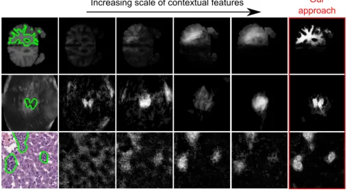
Fig. 1: How to choose the right scale when extracting visual context? This figure illustrates the motivation of this work. For an example label (outlined in green), the maximum range δ at which the visual features are extracted impacts the forest probabilistic output (from left to right: δ = 10, 20, 50, 100). At small scales, fine struc-tures like edges are captured but the lack of long-range information leads to unrealistic predictions. At larger scales, the opposite effect occurs: the approximate position of the structure of interest is correctly inferred, but the level of detail is strongly reduced. Our approach achieves an effective trade-off without computational overhead.
features must be extracted is a crucial problem whose impact on the final per-formance can be enormous (Fig. 1). In general, medical images contain useful information at several complementary scales, going from the local texture around a voxel of interest to the more global anatomical arrangement between organs. For this reason, incorporating multi-scale information during training is of great interest, and several approaches have been proposed to achieve this objective. A common but computationally costly strategy is to perform several independent learning stages at various scales and combine their outputs at prediction time [6, 9, 10]. Geremia et al. [11] explicitly create a hierarchy of supervoxels and refine the representation when necessary during the forest training. Zikic et al. [7] in-corporate the global information via a label prior which is registered to the data at hand and used as an additional image modality. Montillo et al. [3] learn the distribution of the features selected by a preliminary forest, and sample accord-ing to this distribution duraccord-ing the final trainaccord-ing. In spite of their advantages, these approaches present a computational overhead at training or testing time and raise other issues in terms of design, such as having to choose explicitly the different scales to combine.
In this work, we introduce a simple yet effective modification of the for-est training which captures automatically the visual context at the appropriate
scales. Our approach builds on the generic Haar-like features [12] which demon-strated lately high performance for a variety of medical objectives and imaging modalities [3–9]. Instead of sampling Haar-like features uniformly at each node, we sample them sequentially in a fine-to-coarse fashion. This preserves the sim-plicity of the original training as it (i) does not prompt any additional parameter tuning, (ii) leaves by construction the computational training and testing times unchanged, and (iii) does not require any preliminary step such as feature or scale selection. Our method shows consistent improvements with respect to standard approaches on three very different segmentation datasets.
2
Methods
Consider segmentation as a voxelwise1 classification problem, where the goal
is to assign to each voxel p a label y(p). The decision rule predicting y(p) is inferred from a set of labeled examples via a random forest classifier. To do so, the visual content around a voxel has to be quantitatively described by visual features (Sec. 2.1). After recalling the standard framework of classification forests in Sec. 2.2, we introduce in Sec. 2.3 our contribution, i.e. an alternative feature sampling strategy during training which enables an automatic extraction of the visual appearance at the relevant scales.
2.1 Haar-like Features for Segmentation
Like most supervised learning techniques, random forests require a description of training and testing instances (voxels, in our case) through visual features encoding quantitatively the information available for the prediction task. While they can be specifically designed for an application if some domain knowledge is available, a popular and effective approach [3–9] consists in extracting a large number of low-level Haar-like features corresponding to visual cues at offset locations. Each Haar-like feature is characterized by a parameter vector λ ∈ Λ which defines, for each pixel p, a certain type of contextual information xλ(p) ∈ R
as follows. Every parameter vector λ is expressed as λ = (v1, v2, s1, s2 | {z } scale−related , c1, c2, ω | {z } categorical ), (1)
where v1, v2∈ R3are two offset vectors, s1, s2∈ R3+the dimensions of two boxes
respectively attached to each offset, and c1and c2two color channels (or
modali-ties). In each box of size silocated at p+vi(i ∈ {1, 2}), the mean intensity ¯Iiover
the color channel ciis computed. The two quantities ¯I1and ¯I2are combined in a
way determined by a last parameter ω ∈ {diff, binary diff, abs diff, sum}, respectively corresponding to xλ(p) = ¯I1− ¯I2, H( ¯I1− ¯I2),
¯I1− ¯I2
, and ¯I1+ ¯I2.
H denotes the Heaviside function so that H( ¯I1− ¯I2) is the binarized difference
1
between the two mean intensities, which has the useful property of being invari-ant to changes of illumination and contrast. The use of integral volumes [12] allows a fast access to any of these features during training.
2.2 Classification Forests
A random forest is an ensemble of T decorrelated binary decision trees. A de-cision tree is a hierarchically organized set of nodes such that, starting from a root node, each node has exactly 0 or 2 child nodes. A node without children is called a leaf (or terminal node) and contains a posterior probability, whereas each non-terminal node contains a binary decision called splitting function de-signed to route instances towards the left or right child node. At prediction time, a testing instance is sent initially to the root and recursively passed through the tree until it reaches a leaf providing a treewise belief on the instance label. The forest prediction is the average of the T treewise posteriors.
The forest training step consists in the automatic design of the structure and content of each tree from a set of labeled training instances. The T trees are trained in parallel and independently as follows. For a given tree, a set of labeled training samples S is sent to the root node. In the present work, a splitting function is defined as a couple (λ, θ) ∈ Λ × R composed of a visual feature and a threshold. We define the subsets SLλ,θ = {p ∈ S|xλ(p) ≤ θ} and
SRλ,θ = {p ∈ S|xλ(p) > θ} and the information gain generated by this split as
IG(S, λ, θ) = G(S) − S λ,θ L |S| G(S λ,θ L ) − S λ,θ R |S| G(S λ,θ R ), (2)
where G(S) is a purity measure of the set S (the Gini index in our case). In practice, to create a split given a feature λ and a set of samples S, we consider t thresholds θ1, . . . , θtregularly distributed between the extreme values of xλ(p)
observed over all p ∈ S. The threshold providing the highest information gain is retained and defines the information gain IG(S, λ) of the feature λ given S. This greedy threshold optimization is a popular choice due to its computational efficiency [2]. More sophisticated but costlier alternatives have been proposed, e.g. using a differentiable version of the information gain [13].
At each node, the retained splitting function (ˆλ, ˆθ) is determined by drawing randomly N features λ(1), . . . , λ(N ) and keeping the feature ˆλ providing the highest information gain, together with its corresponding best threshold ˆθ. After splitting, SLλ, ˆˆθ and SRλ, ˆˆθ are respectively sent to the left and right child nodes. The process is recursively repeated until a maximum depth is reached or until the number of samples sent to child nodes is too low, in which case a leaf is created. The posterior probability stored at a leaf is defined as the class distribution over the arriving subset of labeled samples.
2.3 Fine-to-Coarse Sequential Feature Sampling
In the standard forest training framework, N candidate features λ(1), . . . , λ(N ) are drawn uniformly and independently at each node. Since each λ(i)is a vector, this is practically achieved by sampling each coordinate λ(i)d of λ(i) uniformly over a predefined set of possible values Λd. In particular, since scale-related
pa-rameters (see Eq.1) are unbounded by definition, an upper limit δ must be set so that offset coordinates take their values in {−δ, . . . , δ} and box dimensions in {1, 3, . . . , δ + 1}. δ encodes the maximum scale at which the visual context is extracted. Deciding on an appropriate value of δ is usually problematic as it strongly impacts the forest prediction (see Fig. 1 for qualitative insights and Ta-ble 1 for quantitative results). In this section, we expose our alternative sampling scheme which alleviates this difficulty at no additional cost.
Instead of sampling the λ(i)independently, we proceed sequentially by letting each candidate feature depend on the previous one. At each node, given an arriving set of training samples S, the feature sampling is conducted as follows: – Sample a first feature λ(1) by setting the scale-related parameters to values corresponding to the finest scale, i.e. 0 for offset coordinates and 1 for box dimensions. The categorical parameters are set randomly.
– At each iteration (for 1 ≤ i ≤ N − 1) :
• Given the current feature λ(i), suggest a slight modification ˜λ of λ(i) by picking at random one of the dimensions λ(i)d (with d ∈ {1, . . . , D} uniformly drawn) and redraw it uniformly among its possible values Λd.
The other components of λ(i)are left unchanged.
• Accept this modification if it does not decrease the information gain. Formally, define λ(i+1)= ˜λ if IG(S, ˜λ) ≥ IG(S, λ(i)), else λ(i+1)= λ(i). This procedure generates N features λ(1), . . . , λ(N ), exactly like the standard uniform sampling technique, and requires the same amount of information gain evaluations so that the computational time is identical by construction. Intu-itively, the chosen initialization of the scale-related parameters corresponds to the finest possible scale which only provides information contained at the voxel of interest. Through the creation of candidate moves ˜λ, changes towards larger scales are then progressively suggested, but only accepted if they convey more information than the current one, in a hill climbing fashion. Hence, the maximum scale δ can be set as high as necessary in practice.
Our approach can also be seen as the design of a Markov chain at each node, where each feature corresponds to a state of the Markov chain and where moves are sequentially suggested from a proposal distribution and accepted if they do not decrease the information gain. This shares some similarities with the Metropolis-Hastings algorithm. The difference lies in the fact that the accep-tance criterion is here deterministic, and that the application of the Metropolis-Hastings algorithm usually requires more iterations than the desired number N of samples to ensure decorrelation between consecutive samples.
3
Experiments
For each experiment, we train T = 10 trees of maximal depth 20 and so that each leaf contains at least 10 training samples. At each node, N = 500 candi-date features are sampled and, for each of them, t = 10 thresholds are tested. Following a bagging strategy, we send to each tree a randomly-chosen fraction of the training data, at a rate of 5% which was experimentally found as a good compromise between accuracy and training time. Our approach is evaluated on three segmentation datasets consisting of MR, 3D ultrasound and histological data. For each of them, we train 5 standard forests with uniform sampling at the scales δ = 10, 20, 50, 100, and 200 pixels respectively. Fig. 1 provides a qualitative intuition on the scale influence as well as an example image from each dataset. Our method using fine-to-coarse feature sampling is trained at the largest scale δ = 200, which includes all the relevant visual information for the segmentation task. As additional baseline, we perform multi-scale prediction by multiplying the posterior probabilities obtained by the 5 standard forests [10]. Since absolute intensity values are unreliable for MR and ultrasound modalities, we also investigate a variant of the feature space which only allows binarized differences (‘Binary’ in Table 1, whereas ‘All ’ denotes the case where the 4 op-eration types are allowed) to guarantee invariance to changes of illumination and contrast. The approximate training times per tree are respectively 10 min (MR), 40 min (ultrasound) and 4 h (histology). The total testing time is 1 min per volume (or large 2D slice). Table 1 shows the mean Dice scores over patients.
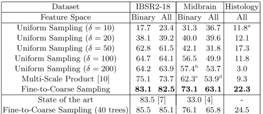
Table 1: Mean Dice scores. To assess the statistical significance of the mean Dice scores, we compared our approach with each baseline by performing a paired sample t-test over the individual Dice scores obtained for each volume (or large slice). All p-values were lower than 0.05, and almost all of them were below 0.001 with only four exceptions. These are marked with a letter (from a to d) in the table below. The cor-responding p-values were respectively 0.0024, 0.033, 0.010 and 0.0077. Finally, we also report the state-of-the-art performance among forest-based methods (when available) and the extension of our method to 40 trees to assess its asymptotical performance.
Dataset IBSR2-18 Midbrain Histology Feature Space Binary All Binary All All Uniform Sampling (δ = 10) 17.7 23.4 31.3 36.7 11.8a Uniform Sampling (δ = 20) 38.1 39.2 40.0 39.6 12.1 Uniform Sampling (δ = 50) 62.8 61.5 42.1 31.8 17.3 Uniform Sampling (δ = 100) 64.7 64.1 56.5 49.9 11.8 Uniform Sampling (δ = 200) 64.2 63.9 57.4b 53.7 3.0 Multi-Scale Product [10] 75.1 73.7 62.3c 53.9d 9.3 Fine-to-Coarse Sampling 83.1 82.5 73.1 63.1 22.3
State of the art 83.5 [7] 33.0 [4] -Fine-to-Coarse Sampling (40 trees) 85.5 85.1 76.1 65.8 24.5
We conclude this section with a short description of the three datasets to-gether with some specific discussions of the results in each case.
1. IBSR2-18 Brain Dataset This is a publicly available2 set of 18 brain
MR scans with up to 32 labeled regions. Since the spacing varies between volumes, we rescale them to obtain an anisotropic spacing of 1 mm. Training voxels are densely collected every 5 mm. A leave-one-out cross-validation is performed. Interestingly, when training a standard forest at the largest scale δ = 200, we recover the performance of an affinely registered label prior which was reported by Zikic et al. [7] (64.2 vs 65.8). This confirms the idea that forests trained at large scales capture the general organization of labels. 2. Midbrain Segmentation in Ultrasound This dataset made available by Ahmadi et al. [14] aims at segmenting the midbrain in 3D transcranial ultrasound. We downsample the volumes by a factor 2, resulting in a spacing of 0.9 mm in all directions. A 7-fold cross-validation is conducted over the 21 volumes. Our method outperforms the state-of-the-art forest-based result [4]. Due to the unreliability of raw intensities in ultrasound data, considering only binary differences is clearly beneficial here (73.1 vs 63.1).
3. Hematopoiesis Quantification in High-Resolution Liver Slices This dataset is a set of high-resolution 2D liver slices extracted from 16 mice, extending the one used by Peter et al. [15]. Here, the objective is to segment hematopoietic cell clusters within the tissue. The image spacing is 1 µm af-ter resizing the images by 2. We perform 4-fold cross-validation. It is a very challenging dataset which is subject to high variability of visual interpreta-tion between experts. While the two other datasets were structured by the skull, hematopoietic cells can be located everywhere so that no label prior can be designed. In spite of these difficulties, a relative improvement of our method in comparison to the baselines can still be observed.
4
Conclusion
In the context of medical image segmentation, we introduced a novel and easy-to-implement alternative for sampling Haar-like features within the random for-est framework. Our method is able to infer automatically the most informative scale at each stage of the training, resulting in an effective combination of local and global context at no additional cost. The experimental validation on three datasets showed the generality and the benefit of the approach.
Acknowledgments This work was partially supported by the Collaborative Research Center 824: “Imaging for Selection, Monitoring and Individualiza-tion of Cancer Therapies”, and by the EU 7th Framework Program project EndoTOFPET-US (GA-FP7/2007-2013-256984). We are very grateful to Kai B¨otzel, Annika Plate and Seyed-Ahmad Ahmadi for kindly providing the mid-brain data through the L¨uneburg Heritage and Deutsche Forschungsgesellschaft
2
(DFG) Grant BO 1895/4-1. We also would like to acknowledge Gabriele Multhoff, Stefan Stangl and Noemi Schworm for making the histological dataset available.
References
1. Breiman, L.: Random forests. Machine Learning (2001)
2. Criminisi, A., Shotton, J.: Decision Forests for Computer Vision and Medical Image Analysis. (2013)
3. Montillo, A., Shotton, J., Winn, J., Iglesias, J., Metaxas, D., Criminisi, A.: Entan-gled decision forests and their application for semantic segmentation of CT images. In Sz´ekely, G., Hahn, H., eds.: IPMI. Volume 6801 of LNCS. Springer, Heidelberg (2011) 184–196
4. Chatelain, P., Pauly, O., Peter, L., Ahmadi, S.A., Plate, A., B¨otzel, K., Navab, N.: Learning from multiple experts with random forests: Application to the segmenta-tion of the midbrain in 3D ultrasound. In Mori, K., Sakuma, I., Sato, Y., Barillot, C., Navab, N., eds.: MICCAI. Volume 8150 of LNCS. Springer, Heidelberg (2013) 230–237
5. Pauly, O., Glocker, B., Criminisi, A., Mateus, D., M¨oller, A., Nekolla, S., Navab, N.: Fast multiple organ detection and localization in whole-body MR dixon sequences. In Fichtinger, G., Martel, A., Peters, T., eds.: MICCAI. Volume 6893 of LNCS. Springer, Heidelberg (2011) 239–247
6. Gauriau, R., Cuingnet, R., Lesage, D., Bloch, I.: Multi-organ localization combin-ing global-to-local regression and confidence maps. In Golland, P., Hata, N., Bar-illot, C., Hornegger, J., Howe, R., eds.: MICCAI. Volume 8675 of LNCS. Springer, Heidelberg (2014) 337–344
7. Zikic, D., Glocker, B., Criminisi, A.: Encoding atlases by randomized classification forests for efficient multi-atlas label propagation. Medical image analysis 18(8) (2014) 1262–1273
8. Kontschieder, P., Dorn, J., Morrison, C., Corish, R., Zikic, D., Sellen, A., D’Souza, M., et al.: Quantifying progression of multiple sclerosis via classification of depth videos. In Golland, P., Hata, N., Barillot, C., Hornegger, J., Howe, R., eds.: MIC-CAI. Volume 8674 of LNCS. Springer, Heidelberg (2014) 429–437
9. Ebner, T., Stern, D., Donner, R., Bischof, H., Urschler, M.: Towards automatic bone age estimation from MRI: Localization of 3D anatomical landmarks. In Golland, P., Hata, N., Barillot, C., Hornegger, J., Howe, R., eds.: MICCAI. LNCS. Springer, Heidelberg (2014) 421–428
10. Lay, N., Birkbeck, N., Zhang, J., Zhou, S.: Rapid multi-organ segmentation using context integration and discriminative models. In Gee, J., Joshi, S., Pohl, K., Wells, W., Z¨ollei, L., eds.: IPMI. Volume 7917 of LNCS. Springer, Heidelberg (2013) 450–462
11. Geremia, E., Menze, B.H., Ayache, N.: Spatially adaptive random forests. In: IEEE 10th International Symposium on Biomedical Imaging (ISBI). (2013) 1344–1347 12. Viola, P., Jones, M.: Robust real-time face detection. IJCV (2004)
13. Montillo, A., Tu, J., Shotton, J., Winn, J., Iglesias, J., Metaxas, D., Criminisi, A.: Entanglement and differentiable information gain maximization. In: Decision Forests for Computer Vision and Medical Image Analysis. Springer (2013) 273–293 14. Ahmadi, S.A., Baust, M., Karamalis, A., Plate, A., Boetzel, K., Klein, T., Navab, N.: Midbrain segmentation in transcranial 3D ultrasound for parkinson diagnosis. In Fichtinger, G., Martel, A., Peters, T., eds.: MICCAI. Volume 6893 of LNCS. Springer, Heidelberg (2011) 362–369
15. Peter, L., Mateus, D., Chatelain, P., Schworm, N., Stangl, S., Multhoff, G., Navab, N.: Leveraging random forests for interactive exploration of large histological im-ages. In Golland, P., Hata, N., Barillot, C., Hornegger, J., Howe, R., eds.: MICCAI 2014. Volume 8673 of LNCS. Springer, Heidelberg (2014) 1–8