Continuous semantic description of 3D meshes

HAL Id: hal-01196895

https://hal.archives-ouvertes.fr/hal-01196895

Submitted on 10 Sep 2015

HAL is a multi-disciplinary open access

archive for the deposit and dissemination of

sci-entific research documents, whether they are

pub-lished or not. The documents may come from

teaching and research institutions in France or

abroad, or from public or private research centers.

L’archive ouverte pluridisciplinaire HAL, est

destinée au dépôt et à la diffusion de documents

scientifiques de niveau recherche, publiés ou non,

émanant des établissements d’enseignement et de

recherche français ou étrangers, des laboratoires

publics ou privés.

Vincent Léon, Nicolas Bonneel, Guillaume Lavoué, Jean-Philippe Vandeborre

To cite this version:

Vincent Léon, Nicolas Bonneel, Guillaume Lavoué, Jean-Philippe Vandeborre.

Continuous

se-mantic description of 3D meshes.

Computers and Graphics, Elsevier, 2016, 54, pp.47-56.

�10.1016/j.cag.2015.07.018�. �hal-01196895�

Vincent L´

eon

, Nicolas Bonneel

, Guillaume Lavou´

e

, and Jean-Philippe Vandeborre

a

_{CRIStAL, UMR 9189, Universit´}

_{e Lille1}

_{CNRS, LIRIS UMR 5205}

c

_Universit´

_{e de Lyon}

d

_{Institut Mines-T´}

_el´

_{ecom / T´}

_el´

_{ecom Lille}

Abstract

We propose a novel high-level signature for continuous se-mantic description of 3D shapes. Given an approximately segmented and labeled 3D mesh, our descriptor consists of a set of geodesic distances to the different semantic labels. This local multidimensional signature effectively captures both the semantic information (and relationships between labels) and the underlying geometry and topology of the shape. We il-lustrate its benefits on two applications: automatic semantic labeling, seen as an inverse problem along with supervised-learning, and semantic-aware shape editing for which the isocurves of our harmonic description are particularly rele-vant.

1

Introduction

With the increasing popularity of digital 3D models in the industry and for the general public, comes an increasing di-versification in the use of this 3D content. New needs are emerging from this diversification: organization of collections, assisted modeling (both for professional and novice users), au-tomatic shape synthesis, auau-tomatic skinning, smart filtering of 3D scenes and so on. These new applications require high-level shape description and understanding, as well as smart shape distance measures. A huge amount of geometric shape descriptors have been introduced by the scientific community over the last 20 years [42] and even very recently [12, 25]. They describe the geometry of the shape either locally or globally, with various degrees of invariance and robustness (with respect to isometry, sampling, etc.). This geometric description is the first step toward understanding and com-paring shapes. However the geometric description remains low-level and may not be sufficient for high-level tasks such as, for instance, retrieving all chair backs in a database of highly heterogeneous chairs. More recently, researchers have tried to derive high-level descriptions of shapes in the form of part labeling, e.g., each face of the 3D shape is labeled as back, leg or seat, in the case of chair models. This high level description may be obtained using supervised learning [19] or by fitting a shape template [22]. Such semantic labeling may be extremely useful in some applications such as database or-ganization. However this approach has the drawback of being constrained by the semantic domain of the database. More-over it defines a hard classification of the mesh elements (one

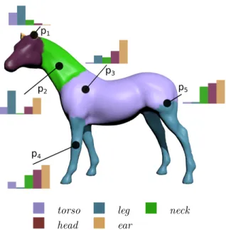
torso leg neck head ear

Figure 1: Illustration of our continuous semantic signature for different points of the Horse model. This signature is built from a prior labeling of the model and consists in the set of geodesic distances to the different semantic parts. For instance, p1 is close to ears and head and far from torso and

legs. This signature conveys the spatially continuous nature of the semantic.

single discrete label for each face among a finite set). As an example, if one considers a labeling of a humanoid model as arm, leg, torso and head, then how can the shoulder be characterized or retrieved? In that context, we introduce a new high level shape representation (illustrated in Figure 1) which encodes both semantic and geometric information, in the form of a multidimensional real-valued vector. The idea is simple: each vertex is characterized by its geodesic distances to every semantic part of the object. This rich and continuous information allows us to much better characterize the seman-tic context of a vertex, as well as the relationships between semantic parts. Applications of this new representation are numerous: shape labeling, skinning, geometry transfer, as-sisted modeling and so on.

The rest of this paper is organized as follows: section 2 describes the related work about 3D shape description and understanding. Then, section 3 presents our descriptor and its properties. Finally, we present two applications: 3D-mesh

labeling (section 4) and geometric detail transfer (section 5).

2

Related Work

An incredible amount of work has been devoted during the last 20 years on 3D shape description and representation. This topic is involved in many computer graphics areas such as shape retrieval, segmentation or shape correspondence. In this section, we first cover approaches that are most closely related to our semantic context representation. We refer the reader to recent surveys for more in-depth discus-sions [42, 46, 48]. We then examine the relevant work in shape editing, which is one of the main applications of our representation.

2.1

Shape description

A great variety of geometric shape descriptors have been in-troduced for the purpose of shape representation, understand-ing and retrieval. The earliest ones were global – they repre-sent a shape by a single signature. The first global descrip-tors were only robust to rigid deformations (e.g., spherical harmonics [14]), while more recent ones are also invariant to non-rigid deformations like near-isometries. These latter de-scriptors include spectral embeddings [32, 33] or histograms of local shape descriptors [30, 15] including bag-of-word mod-els [8, 28]. Local descriptors associate one signature per ver-tex, face or local region of a 3D shape; they include simple differential quantities (e.g., curvature), shape diameter [15], histogram of gradients [50], the heat kernel signature [39], shape context [25] or spin images [12]. In contrast to these ge-ometric descriptors, topological representations are also very popular for shape retrieval and understanding [4]. They in-clude mostly graph representations like Reeb graphs [6, 5, 43] or simpler region adjacency graphs obtained from a segmen-tation [35].

These shape descriptors (both for geometry and topol-ogy) are low-level and thus do not relate to the shape se-mantics in any way. However, they may be used to derive high-level representations like a semantic labeling. This gap from low-level to high-level description may be filled using manual annotations combined with an ontology describing the semantic domain, as proposed by Attene et al. [2]. To get rid of these manual interactions, recent data-driven tech-niques [19, 29, 44, 47] benefit from the availability of large semantically annotated 3D data collections to infer semantic labels from large sets of low-level descriptors using supervised learning. Co-analysis [17, 36, 45] can also infer consistent la-bels within a collection. In slightly different ways, Kim et al. [22] learn and then fit a shape template to obtain a consis-tent labeling of a whole model collection, while Laga et al. [27] and Zheng et al. [52] analyze the relationships between parts for the same purpose. Such semantic labeling is perfectly suited for several high level applications such as database ex-ploration [13] or modeling by part assembly [10, 3]. However it has two major drawbacks: (1) it is limited to a pre-defined ontology (i.e., a finite set of predetermined labels) and (2) it does not convey the continuous nature of semantics. For instance, for a human being or an animal, there is no strict

semantic boundary between a leg and the torso but there exist regions that belong to both parts in certain proportions.

Our representation solves these issues by encoding the se-mantic in a continuous way, as well as geometric and topolog-ical information in one single local multidimensional descrip-tor.

2.2

Shape editing

Reusing existing geometry to synthesize new models is an important challenge in computer graphics. The objective is to ease the designers work and speed up the production of these 3D models. Two main classes of methods have been proposed so far: part assembly and geometry cloning.

Part assembly [10, 26, 20, 49, 18, 16] consists in gener-ating (automatically or using an adapted interface) new 3D models by gluing together existing parts from a pre-processed database. The main weakness of these techniques is that they rely on a prior segmentation/labeling and thus their degree of freedom is limited by the pre-defined semantic domain. For instance it is impossible to glue an ear on the head of a 3D model, if these two components do not possess different labels in the database.

On the other side of the spectrum are geometry cloning tools which do not consider any semantic information or prior segmentation, but rather consist in fully manual cut-and-paste operations, either conducted on large geometric parts [34] or on surface details [38, 41]. The main drawback of these ex-isting works is that the precise location of the part or details to be transferred from a source to a destination model has to be manually determined – on both the source and the desti-nation. However, such process could really benefit from se-mantic information. For instance the geometric texture of a shoulder region from a source object could be automatically pasted on the shoulder region of the destination model.

Our continuous semantic representation allows for bridging the gap between part assembly (which is too constrained by a prior segmentation) and geometry cloning (which is fully manual). It intrinsically encodes a smooth semantic map-ping between two shapes, that allows for a smart automatic geometry transfer. Note that such correspondence may also be computed using surface mapping algorithms [21, 1]. How-ever, these algorithms are clearly not suited for the real-time interactions required by design applications.

3

Continuous Semantic Description

Given an approximately segmented and semantically labeled mesh, our descriptor consists in a set of geodesic distances to the different labels. This section describes in more details this new, semantic, local descriptor, which accurately con-veys the spatially continuous (contrary to uncertain) nature of a mesh labeling as well as topological relationships within the mesh. Good properties of this descriptor are illustrated through various experiments.

3.1

Semantic Sampling

To compute our descriptor, the first step is to sparsely sample points on the mesh. The benefit of this is to avoid

the need of a precise segmentation, which makes it robust against segmentation mistakes inherent to most methods. As such, we do not assume a particular segmentation method and just assume we are provided with a coarsely segmented mesh, along with a semantic labeling for each segment. By semantic labeling, we assume, for instance, that a single label “leg” is given to the four legs of a quadruped, rather than a different label for each leg, and that this labeling is consistent within a database of similar objects. Many efficient algorithms are now able to compute such consistent segmentation and labeling over a database of 3D models [19, 44, 17, 36, 29, 45, 22, 47]. In practice, in the examples of this paper, we consider the models from the Princeton segmentation benchmark [11], segmented and labeled by the method of Kalogerakis et al. [19]. Examples of this labeling are illustrated in Figure 2.

Figure 2: Illustration of some classes of models (labeled by [19]) that we consider in the examples of this paper: Hu-man (8 labels), Armadillo (11 labels), FourLeg (6 labels) and Airplane (5 labels).

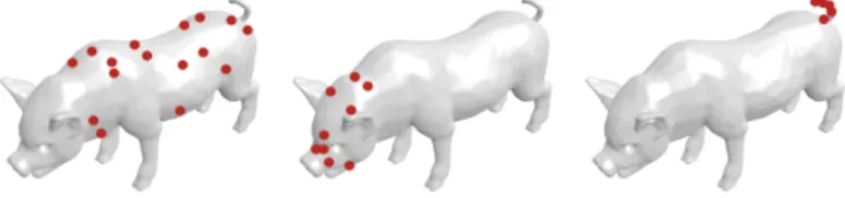
We consider an adaptive sampling strategy. For each label, we determine a number of samples proportional to the area of that label over the mesh (we add a minimum number of samples to avoid under-represented labels such as the ears or tail). We then randomly select faces according to their area (and label) and sample within these faces. We use 10 + 100 × area(`)/area(mesh) samples per label (where area(`) is the total area of the label `). A visualization of some sampled labels can be seen in Figure 3.

Figure 3: Our label sampling strategy. Left to right: body, head, tail.

3.2

Semantic Shape Signature

For each label `, we have obtained a set of samples S` as

described in Section 3.1. Our descriptor, denoted d, depends on a predefined set of labels L, which corresponds to the entire

collection of labels present in a mesh database. For a given point p on the mesh, the descriptor is computed as a vector of |L| elements. Each element of the vector d(p), denoted d`(p),

describes the relation between the point p and the label `. In many cases, and in particular for heterogeneous databases, a single model will only possess a subset of the entire set of labels L. This makes the descriptor sparse, and some elements of the descriptor will just be undefined.

The scalar d`(p) is computed as the geodesic distance from

p to the closest point in S`, denoted g(p, S`). As the points

in S` may belong to different segments, this makes our

de-scriptor invariant to the number of occurrences of a label in a shape. For instance, if we consider a dataset of human mod-els, our descriptor would contain (among other relationships) the geometric relationship between the points of the models and the nearest of the two arms. Intuitively, the descriptor indicates that a point on the shoulder of a human will be close to the label arm but far from the label leg, in term of geodesic distance. This is in contrast to probabilistic approaches which would consider a point on the shoulder more likely to belong to the arm than the leg. A probabilistic approach based on geometric features is unable to tell that a point on a shoulder is actually in-between the arm and the head, but can only assign probabilities based on resemblance. Further, our use of geodesic distances makes our descriptor robust to changes in pose and sampling, as shown in Figure 5.

The descriptor is thus computed as: d(p) = {d`(p), ` ∈ L}

d`(p) = min s∈S`

(g(p, s)) (1)

where g is the geodesic distance. When a label ` is not repre-sented in a shape, a default value d`= ∞ is used. In practice,

we compute an exact geodesic distance with the algorithm of Surazhsky et al. [40].

Figure 1 illustrates our descriptor for a few points of a mesh. This signature smoothly encodes the semantic information and its topology (i.e., relationships between labels) as well as geometric information. Unlike a simple labeling, it is able to easily discriminate different points having the same label but different positions (e.g. P4 and P5). Figures 4 and 5

illus-trates the d` scalar field for different labels `. Once again,

these figures show that our signature describes a continous semantic information, much richer than a simple labeling.

3.3

Properties

Our signatures exhibits several useful properties detailed be-low.

3.3.1 Robustness

Since we compute exact geodesic distances on the surface, as well as an adaptive semantic sampling, our descriptor is in-variant to the mesh resolution, as can be seen in Figure 6. It is also very robust to near-isometric deformations like skeletal articulations as illustrated in Figure 5. Further, when increas-ing the number of samples, our descriptor converges toward a set of geodesic distances to segment boundaries – which would

foot lowerleg upperleg torso head upperarm lowerarm hand

Figure 5: Visualization of d`(p) for two meshes of the Human category from the Princeton Benchmark [11].

body rudder wing

Figure 4: Visualization of d`(p) (blue to red for low to high)

for two meshes of the Airplane category from the Princeton Benchmark [11].

not be robust against small segmentation mistakes. Our sam-pling strategy hence enforces robustness against segmentation inaccuracies. In practice, within a segment with label `, the distance corresponding to that label can be non-zero. How-ever, we did not find this to be problematic in our experi-ments.

3.3.2 A semantic-aware distance

A simple L2 _{distance in our signature space defines a new}

semantic-aware metric over the surface. Figure 7 shows uni-formly sampled isocurves of the distance field from a point on the right knee to the rest of the human body. For comparison we also illustrate the geodesic distance field. Our metric well reflects the semantic distance.

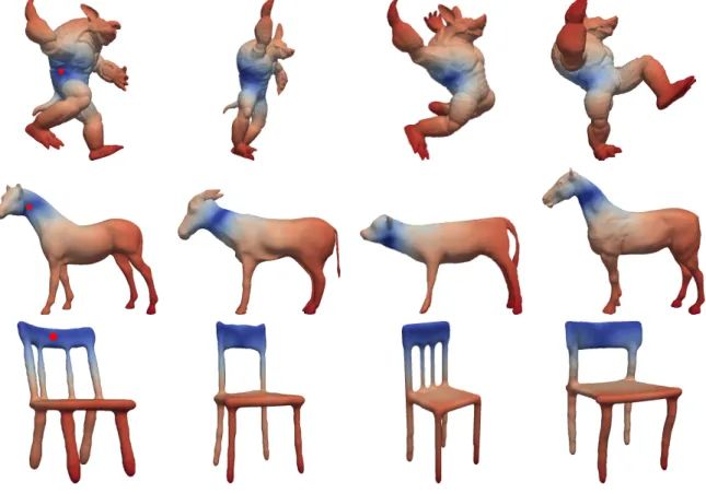
Figure 8 illustrates the use of the previously defined metric for computing correspondences between different models. In both examples (Armadillo, FourLeg and Chair classes), we selected a point (in red) on the first model, and computed the L2 distance in descriptor space, from this point to ev-ery vertices of evev-ery models (including itself). We see that

hand lowerleg

Figure 6: Visualization of d`(p) on two labels, with different

mesh resolutions (11015 and 2639 vertices respectively)

an accurate correspondence is found between models, illus-trated by the semantic similarity between blue areas, even in the case of strong pose changes (Armadillo) or shape varia-tions (FourLeg,Chair ). To summarize, starting from a coarse corresponding labeling (see Figure 2), our signature defines a dense correspondence between the models. This correspon-dence may be very useful for many applications such as part-in-shape retrieval and selection, as well as mesh editing and geometry transfer. Existing work on dense mesh correspon-dence such as the work of Ovsjanikov et al. [31] are based on local geometry desciptors, and does not account for any semantic information.

The top row in Figure 9 further illustrates the use of the L2distance in our descriptor space for models of the Human

class. The selected point on the elbow of the first model is matched to the others. On the second row, faces are described using the 608 geometric unary features proposed by Kaloger-akis et al. [19] and the matching is performed using the L2

ob-Figure 8: Correspondence between several models, computed using our signature. For each class (Armadillo, FourLeg and Chair

) we compute the L2 signature distance from the red point to every vertices of every models of the class (illustrated in a

blue to red logarithmic scale). The semantic similarity between the blue regions in each row illustrates that an accurate correspondence is found between models.

Geodesic distance L2signature distance

Figure 7: Distance field from a point on the knee to the rest of the model, computed with a simple geodesic distance (left ) and with the L2 distance in our signature space (right ). We

observe than our signature-based metric integrates both geo-metric and semantic information, as it captures variations of the geodesic distances to all semantic labels.

tained in this latter case illustrates the fact that even a very large set of geometric features cannot compete with our de-scriptor in term of semantic correspondence.

3.3.3 Descriptive power

Our signature may also be useful to describe segments (i.e. parts of a mesh). In that case, each segment is described by a collection of |L| histograms, obtained by uniformly sampling the segment and accumulating each sample’s signature. In Figure 10, we depict the repartition of the segments of two classes from the Princeton Benchmark [11] previously labeled by [19], obtained by multi-dimensional scaling (MDS) applied on a signature difference between segments. This signature difference is defined as the sum of the Earth Movers distances between histograms. Each point represents a segment, with the color corresponding to the label. The apparent clustering of points according to their labels appears to validate the semantic quality of the L2 descriptor distance. Besides this correct visual clustering, we observe that our descriptor also provides insights about the geometry and the topology of the segments which may bring valuable information. For instance the engines of the Airplane class are not clustered together because engines have a different context: some of them are attached to the nose of the plane, some are attached on the side, while other may be attached to the wings. Interestingly, the respective positions of the clusters provide information about the relationships between labels. For instance the body cluster of the Airplane class is at the center of the other labels, like the torso for the Human class. As another example, the lowerArm cluster is at the opposite of the foot cluster. We

Figure 9: Correspondence between models from the Human class, comparison with the features from [19]. Top row: L2

distance in our signature space. Bottom row: L2 distance on

the geometric descriptor set from [19] (608 dimensions).

will see in the next section that this rich descriptive power may be useful for automatic region labeling.

4

Application to Semantic Labeling

As detailed in section 3, our descriptor requires a complete labeling of the mesh, which does not seem suitable at first for a mesh labeling application. In this section, we demon-strate that a combinatorial optimization step along with su-pervised learning allows for the semantic labeling of an unla-beled shape.

As our descriptor describes the relationship between the geometry and labels in a set of shapes, we consider the la-beling task as an inverse problem. Specifically, we find the best labeling maximizing the probability of a label, given the descriptor, outputted by a random forest classifier given a pre-labeled dataset.

4.1

Labeling as a Inverse Problem

We consider an input 3D model Q with m unlabeled segments, that may come from any segmentation algorithms [51, 23]. By using a database of segmented and labeled models, we infer the labels of Q. We proceed in two steps: the training step, for which a random forest classifier learns from the labeled database, and the inference step which estimates the most probable labeling of the input model.

4.1.1 Training

For every shape in the training set, we extract a set of source points S` for each label ` ∈ L using the method described in

Section 3.1.

We perform supervised learning by considering a feature vector for each segment of each model associated with its ground-truth label. The feature vector consists of a collection of |L| histogram statistics. Specifically, we uniformly sam-ple the input model and compute our descriptor d for all the

samples according to the ground-truth labels. For each label `, we bin the descriptors d`at these sample points to produce

a histogram, and compute their mean, standard deviation, skewness and kurtosis. These statistical features are classi-cally used for describing distributions [37]. We thus obtain a feature vector of size 4 × |L|. If the label is not represented in the shape, the corresponding element of the feature vector is not used for this shape.

With this training set, we train a multi-class Random For-est Classifier [7] on the ground-truth labels.

4.1.2 Inference

Given an input model with m segments, we wish to label it using the previously trained classifier. However, we recall that our descriptor requires a per-segment labeling: we tackle this challenge by evaluating hypotheses on possible labelings.

First, we sample each segment si by a set of source point

Pi. We then compute a matrix M of m × m histograms. The

element Mi,j of the matrix contains a histogram of shortest

geodesic distances between all sample points Piand their

cor-responding closest point in Pj.

We then evaluate a candidate labeling using our classifier. For every segment si of the input model, the classifier

out-puts the probability P (label(si) = `) of the segment si to be

assigned the label `. We determine a score for a complete labeling hypothesis L by taking the product of all these prob-abilities for each segment

P (L) =

m

Y

i=0

P (label(si) = `) (2)

While this assumes labels are independent of each other, this simplifying assumption works reasonably well for our purpose (see Section 4.2). A statistically correct approach would be intractable since descriptors (and hence P (label(si) for all

seg-ments) rely on the label of all other segments.

We generate the combinatorial, yet reasonably small, set of possible labelings, and retain the one maximizing this score. While we attempted more heuristic approaches such as simu-lated annealing, this solution was significantly degrading the quality of our results.

4.2

Results

We test our labeling method on the Princeton Segmentation Benchmark [11] which contains 19 categories, each of 20 ob-jects, ranging from humans to man-made objects. We use the segmentation method and ground truth of Kalogerakis et al. [19]. In practice, there are |L|m _{possible labelings. This}

remains tractable within the benchmark (each category con-tains on average |L| = 5 labels and m = 7 segments per object, yielding around 80000 evaluations). Our unoptimized implementation takes 5 minutes for training our classifier on an entire class of 20 meshes. The inference takes between 56 seconds (for Glasses) and 30 hours (for Armadillos which have the largest number of labels and segments), and the me-dian time is 18 minutes. Parallelization and simple heuristics on label cardinality can be used to lower the inference time. For instance, early experiments shown a three-fold speedup on the Bird class by assuming the cardinality of each label

body rudder engine

wing stabilizer

(a) Airplanes

head torso upperLeg lowerLeg

hand foot upperArm lowerArm

(b) Humans

Figure 10: Multi-dimensional scaling analysis of the segments of the Airplane and Human categories from the Princeton Benchmark [11]

known in advance (e.g., two wing segments, one tail etc.), without loss of accuracy. This heuristic could be considered when the mesh to be segmented is consistent with the training database.

We demonstrate the accuracy of our method using a leave-one-out cross-validation on each category of object. This ex-periment assumes the class of the object is known, but this restriction can be alleviated at the expense of larger inference times. In Table 1, we report the number of labels |L| consid-ered for each category, and the percentage of faces correctly la-beled by our method. We also present, for comparison, results obtained using a simple geometric descriptor (an histogram of Shape Indices [24] combined with segment areas) and results obtained using the large feature vector from Kalogerakis et al. [19]. In this latter case, as for our signature, we feed the random forest classifier with the mean, standard deviation, skewness and kurtosis of the distributions of the 608 unary features resulting in a 2432-dimensional feature vector. We also present results when combining this large set of geometric features with our signature. Results show that the combina-tion of geometric and semantic informacombina-tion provides the best results; however, our descriptor alone (which has an average of 20 dimensions) performs reasonably well given its low di-mensionality – albeit less than the high-dimensional geometric descriptor of Kalogerakis et al.

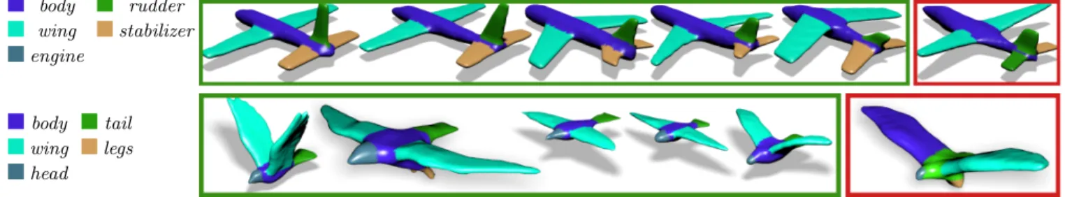
In Figure 11, we illustrate labeling results on the Air-plane and Bird classes of the Princeton Segmentation Bench-mark. The last examples are not correctly labeled, when com-pared to the ground truth labels provided by Kalogerakis et al. [19].For one plane, a stabilizer is labeled as rudder, since the two parts are similar in both geometry and semantic con-text.

To further assess the robustness of our method with re-spect to inaccurate segmentations, we used our technique to label under and over-segmented meshes (three birds and three cups), compared to the training database (figure 12). We merged the body and head segments of two bird meshes and connected the two wings in one of them. We also over-segmented another bird and three cups into seven parts (the training dataset consists in two segments only). For under-segmented meshes our automatic labeling often remains

cor-Category # labels ours [24] [19] ours+[19] Airplane 5 87.6 36.5 96.0 98.5 Ant 5 83.0 28.0 99.2 99.2 Armadillo 11 76.3 20.3 98.1 98.1 Bearing 6 57.1 2.0 85.2 84.1 Bird 5 87.5 3.8 95.4 94.0 Bust 8 65.4 2.6 68.1 67.7 Chair 4 59.0 1.7 99.7 99.7 Cup 2 92.1 87.5 95.1 95.1 Fish 3 82.4 78.2 100 90.5 FourLeg 6 80.0 25.0 97.8 97.7 Glasses 3 81.1 64.8 100 97.4 Hand 6 91.1 4.9 87.5 90.9 Human 8 79.3 13.2 92.1 92.0 Mech 5 75.9 14.9 84.7 87.6 Octopus 2 78.6 52.3 55.0 100 Plier 3 61.8 12.9 100 100 Table 2 84.3 89.2 97.8 97.8 Teddy 5 70.2 13.8 100 100 Vase 5 77.2 1.2 85.0 93.8 Average 5 77.3 29.1 91.4 93.7

Table 1: Performance on the Princeton Segmentation Bench-mark (ground-truth from [19]). For each category, we show the number of labels and percentage of correct labels per face using our 20-dimensional descriptor, simple geometric descriptors (segment area and Shape Indices [24]), 2432-dimensional statistical moments from the 608-2432-dimensional unary geometric potentials of Kalogerakis et al. [19], and com-bining our descriptor with these geometric potentials. Com-bining both geometry and semantic gives the best result, but our semantic descriptor alone achieves reasonable success given its low-dimensionality.

body rudder wing stabilizer engine body tail wing legs head

Figure 11: Labeling results for the Airplane and Bird classes of the Princeton Segmentation Benchmark. Green (resp. red) boxes represent correct (resp. incorrect) labeling.

Figure 12: Labeling results using segmentations inconsistent with the training set. Green (resp. red) boxes represent cor-rect (resp. incorcor-rect) labelings. On the top-left, birds are under-segmented: the body and head are merged or the wings are connected. Given this under-segmentation, the labeling is correct. On the top-right, the bird is over-segmented into 7 parts which results in parts of the wings being misclassi-fied as body. In the bottom row, cups are over-segmented into seven segments, which can result in part of the handle to be misclassified as inside (bottom right). In general, under-segmentations do not pose particular problems for our label-ing, while problems may occur with over segmentations.

rect, while over-segmentations occasionally misclassify seg-ments (right column).

5

Application to Mesh Editing

In this section, we illustrate the use of our descriptor for semantic-aware mesh editing purposes, such as the addition of geometric details or filtering. The continuous semantic na-ture of our descriptor and the semantic meaning of its asso-ciated L2 _{metric allow to obtain natural-looking shape}

mod-ifications. We present here three usage scenarios:

1. The user selects a semantic label (e.g. upper leg) and the geometric modification is applied to the whole re-gions for which the corresponding d` is the smallest

di-mension of the descriptor. On the border of the region, the strength of the modification decreases as the corre-sponding dimension of the descriptor, normalized over all dimensions, increases.

2. The user selects a point on the mesh, and the geometric modification is applied around this point and decreases according to the L2 distance in the descriptor space.

3. The user selects a point and an isoline (produced using the L2 _{metric), and then the modification is applied on}

the whole region bounded by the isoline. Once again the strength is decreased as we go further from the selected isoline (in the descriptor space). Thanks to the isolines, the user can very easily selects a semantic region not ini-tially defined in the prior labeling, such as the shoulder, in the case of a humanoid.

In these three scenarios, we have used a Gaussian function N (µ = 0, σ2_{) of the distances, with σ}2 _{= 50 when applying}

on descriptor-space L2 _{distance and σ}2 _{= 30 when we use}

only one geodesic distance. In all scenarios, distances are normalized by the size of the mesh.

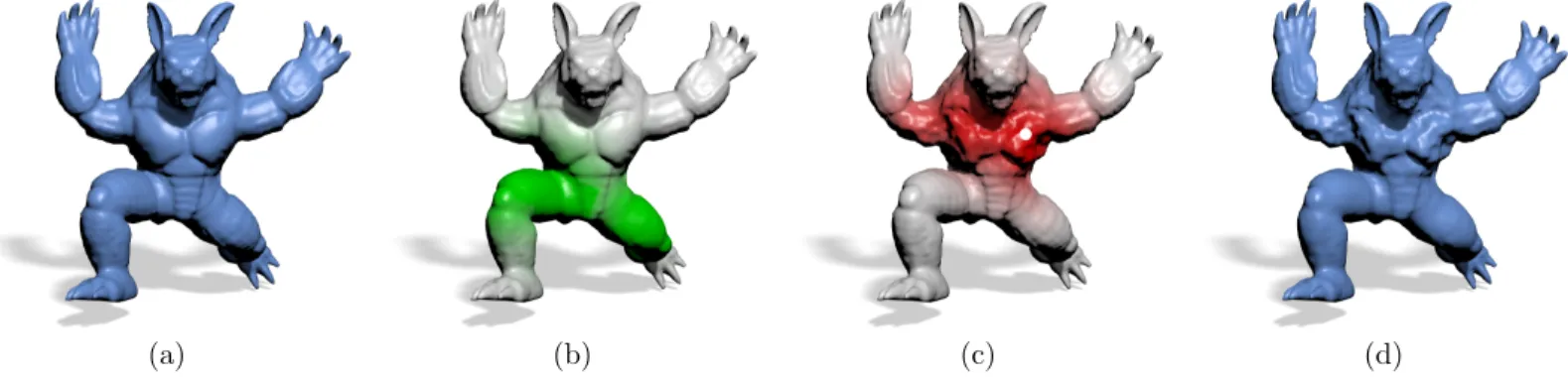
Scenarios 1 and 2 are illustrated in Figure 13 for which we apply an additive Perlin noise on the torso and a smoothing on the upper legs of an Armadillo model. For the smooth-ing operation, we select the upper leg label (scenario 1). We thus only use one dimension of our descriptor: we smooth the whole area for which the smallest dimension corresponds to this label. The strength of the smoothing is represented by the opacity of the green color.

For the noise addition we select the point highlighted in white (scenario 2) then the modification is applied around this point according to the L2 _{signature distance. We can see that the}

procedural noise has been naturally spread all over the torso region. Regions such as the hands or the head remain intact. Figure 13 (d) illustrates the model after both modifications. As another example, in Figure 14 we select the red point on the shoulder of a humanoid model as well as the isoline illus-trated in red (scenario 3). We then extrude all vertices within the isolines. Note that since we are measuring distances in the descriptor space, vertices on the other shoulder are automat-ically extruded as well; this symmetry comes for free thanks to the semantic information.

6

Conclusion

We have described a simple yet effective shape signature, based on geodesic distances to semantic labels. Unlike a sim-ple labeling, this descriptor conveys the spatially continuous

(a) (b) (c) (d)

Figure 13: Application to mesh editing - (a) Original Armadillo model - (b) Result after Laplacian smoothing when selecting the upperleg label - (c) Noise added by selecting a point (in white) on the torso - (d) Final Armadillo model after both smoothing and noise addition. Note that the distance in our descriptor space allows a smooth naturally-looking decreasing of the strength of the geometric modifications (illustrated by the opacity of the colors).

(a) (b)

Figure 14: Application to mesh editing - (a) Original Human model - a point (in red) is selected on the shoulder/upperarm region of the original model as well as the isolines (in red) -(b) Vertices bounded by the isolines are extruded with smooth transition at the borders (illustrated by the opacity of the color). Note that the editing is symmetrical due to the sym-metry of the labeling.

nature of the semantic as well as its topology (i.e. the rela-tionships between semantic parts). We have demonstrated its benefit on two applications: automatic semantic labeling and semantic-aware shape editing.

In the future, we plan to exploit our shape signature for data-driven shape editing and design (i.e., using a database of existing preprocessed models to support the design/editing). Producing tools to assist and support the graphic designer in her modeling task becomes a fundamental research issue since the production of massive amount of 3D content is now a major concern for the global production chain of digital en-tertainment products. In this work, we showed that our shape signature was perfectly suited for semantic-aware shape ing. To create a complete system for data-driven shape edit-ing, we now plan to devise complementary tools like a smart user interface for semantic-aware mesh selection. Some recent user interfaces dedicated to innovative 3D content creation [9] may be inspiring for this task.

Besides shape editing, we would also like to explore other applications like automatic skinning and database explo-ration. We believe that our descriptor may be highly relevant in such cases where semantic is a key ingredient.

Acknowledgement

This work is supported by the ANR (Agence Nationale de la Recherche, France) through the CrABEx project (ANR-13-CORD-0013)1.

References

References

[1] Noam Aigerman, Roi Poranne, and Yaron Lipman. Lifted bijections for low distortion surface mappings. ACM Transactions on Graphics, 33(4), 2014.

[2] Marco Attene, Francesco Robbiano, and Michela Spag-nuolo. Characterization of 3D shape parts for seman-tic annotation. Computer-Aided Design, 41(10):756–763, 2009.

[3] Melinos Averkiou, Vladimir G. Kim, Youyi Zheng, and Niloy J. Mitra. ShapeSynth: Parameterizing model col-lections for coupled shape exploration and synthesis. Computer Graphics Forum, 33(2):125–134, May 2014.

[4] S Biasotti, L De Floriani, B. Falcidieno, P. Frosini, D. Giorgi, C. Landi, L. Papaleo, and M. Spagnuolo. De-scribing shapes by geometrical-topological properties of real functions. ACM Computing Surveys, 40(4), 2008.

[5] S. Biasotti, D. Giorgi, M. Spagnuolo, and B. Falci-dieno. Reeb graphs for shape analysis and applications. Theoretical Computer Science, 392(1-3):5–22, February 2008.

[6] Silvia Biasotti, Simone Marini, Michela Spagnuolo, and Bianca Falcidieno. Sub-part correspondence by struc-tural descriptors of 3D shapes. Computer-Aided Design, 38(9):1002–1019, September 2006.

[7] Leo Breiman. Random forests. Machine Learning, 45(1):5–32, 2001.

[8] Alexander M. Bronstein, Michael M. Bronstein, Leonidas J. Guibas, and Maks Ovsjanikov. Shape google: Geometric words and expressions for invariant shape re-trieval. ACM Transactions on Graphics, 30(1):1–20, Jan-uary 2011.

[9] Siddhartha Chaudhuri, Evangelos Kalogerakis, Stephen Giguere, and Thomas Funkhouser. Attribit: Content creation with semantic attributes. In ACM Symposium on User Interface Software and Technology, pages 193– 202, 2013.

[10] Siddhartha Chaudhuri, Evangelos Kalogerakis, Leonidas Guibas, and Vladlen Koltun. Probabilistic reasoning for assembly-based 3d modeling. ACM Transactions on Graphics, 30(4):35:1–35:10, July 2011.

[11] Xiaobai Chen, Aleksey Golovinskiy, and Thomas Funkhouser. A benchmark for 3D mesh segmentation. ACM Transactions on Graphics, 28(3), 2009.

[12] T Darom and Y Keller. Scale Invariant Features for 3D Mesh Models. IEEE Transactions on Image Processing, 21(5):2758 – 2769, January 2012.

[13] Noa Fish, Melinos Averkiou, Oliver van Kaick, Olga Sorkine-Hornung, Daniel Cohen-Or, and Niloy J. Mi-tra. Meta-representation of shape families. ACM Transactions on Graphics, 33(4):1–11, July 2014. [14] Thomas Funkhouser, Patrick Min, Michael Kazhdan,

Joyce Chen, Alex Halderman, David Dobkin, and David Jacobs. A search engine for 3D models. ACM Transactions on Graphics, 22(1):83–105, 2003.

[15] Ran Gal, Ariel Shamir, and Daniel Cohen-Or. Pose-oblivious shape signature. IEEE Transactions on Visualization and Computer Graphics, 13(2):261–71, 2007.

[16] Xuekun Guo, Juncong Lin, Kai Xu, and Xiaogang Jin. Creature grammar for creative modeling of 3D monsters. Graphical Models, 76(5):376–389, September 2014. [17] Qixing Huang, Vladlen Koltun, and Leonidas Guibas.

Joint shape segmentation with linear programming. ACM Transactions on Graphics, 30(6), 2011.

[18] Arjun Jain, Thorsten Thorm¨ahlen, Tobias Ritschel, and Hans-Peter Seidel. Exploring shape variations by 3d-model decomposition and part-based recombina-tion. Computer Graphics Forum, 31(2pt3):631–640, May 2012.

[19] E Kalogerakis and Aaron Hertzmann. Learning 3D mesh segmentation and labeling. ACM Transactions on Graphics, 29(4), 2010.

[20] Evangelos Kalogerakis, Siddhartha Chaudhuri, and Daphne Koller. A Probabilistic Model for Component-Based Shape Synthesis. ACM Transactions on Graphics, 2012.

[21] VG Kim, Y Lipman, and Thomas Funkhouser. Blended intrinsic maps. ACM Transactions on Graphics, 30(4), 2011.

[22] Vladimir G. Kim, Wilmot Li, Niloy J. Mitra, Siddhartha Chaudhuri, Stephen DiVerdi, and Thomas Funkhouser. Learning part-based templates from large collections of 3D shapes. ACM Transactions on Graphics, 32(4), July 2013.

[23] Oscar Kin-Chung Au, Youyi Zheng, Menglin Chen, Pengfei Xu, and Chiew-Lan Tai. Mesh Segmentation with Concavity-Aware Fields. IEEE Transactions on Visualization and Computer Graphics, 18(7):1125–1134, July 2011.

[24] Jan J. Koenderink and Andrea J. van Doorn. Sur-face shape and curvature scales. Image Vision Comput., 10(8):557–565, October 1992.

[25] I. Kokkinos, M. M. Bronstein, R. Litman, and a. M. Bronstein. Intrinsic shape context descriptors for de-formable shapes. IEEE Conference on Computer Vision and Pattern Recognition, pages 159–166, June 2012. [26] Vladislav Kreavoy, Dan Julius, and Alla Sheffer.

Model composition from interchangeable components. Computer Graphics and Applications, pages 129 – 138, 2007.

[27] Hamid Laga, M Mortara, and M Spagnuolo. Geome-try and context for semantic correspondences and func-tionality recognition in man-made 3D shapes. ACM Transactions on Graphics, 32(5), 2013.

[28] G Lavou´e. Combination of bag-of-words descriptors for robust partial shape retrieval. The Visual Computer, 28(9):931–942, 2012.

[29] J Lv, X Chen, J Huang, and H Bao. Semi-supervised Mesh Segmentation and Labeling. Computer Graphics Forum, 31(7):2241–2248, 2012.

[30] R Osada and T Funkhouser. Shape distributions. ACM Transactions on Graphics, 21(4):807–832, 2002.

[31] Maks Ovsjanikov, Mirela Ben-Chen, Justin Solomon, Adrian Butscher, and Leonidas Guibas. Functional maps: a flexible representation of maps between shapes. ACM Transactions on Graphics, 31(4):30:1–30:11, 2012. [32] M Reuter, F Wolter, and N Peinecke. Laplace-Beltrami spectra as Shape-DNA of surfaces and solids. Computer-Aided Design, 38(4):342–366, April 2006. [33] RM Rustamov. Laplace-Beltrami eigenfunctions

for deformation invariant shape representation. In Eurographics symposium on Geometry processing, pages 225 – 233, 2007.

[34] Ryan Schmidt and Karan Singh. Meshmixer: an interface for rapid mesh composition. In SIGGRAPH Talks, 2010. [35] Konstantinos Sfikas, Theoharis Theoharis, and Ioannis Pratikakis. Non-rigid 3D object retrieval using topologi-cal information guided by conformal factors. The Visual Computer, 28(9):943–955, April 2012.

[36] Oana Sidi, O. van Kaick, Y. Kleiman, H. Zhang, and D. Cohen-Or. Unsupervised co-segmentation of a set of shapes via descriptor-space spectral clustering. ACM Transactions on Graphics, 30(6), 2011.

[37] Patricio Simari, Binbin Wu, Robert Jacques, Alex King, Todd McNutt, Russell Taylor, and Michael Kazhdan. A statistical approach for achievable dose querying in imrt planning. Medical Image Computing and Computer Assisted Intervention, pages 521–528, 2010.

[38] O Sorkine, D Cohen-Or, and Y Lipman. Laplacian sur-face editing. Symposium on Geometry Processing, 2004. [39] Jian Sun, Maks Ovsjanikov, and Leonidas Guibas. A Concise and Provably Informative Multi-Scale Signature Based on Heat Diffusion. Computer Graphics Forum, 28(5):1383–1392, July 2009.

[40] Vitaly Surazhsky, Tatiana Surazhsky, Danil Kirsanov, Steven J. Gortler, and Hugues Hoppe. Fast exact and approximate geodesics on meshes. ACM Transactions on Graphics, 24(3):553–560, July 2005.

[41] Kenshi Takayama, Ryan Schmidt, Karan Singh, Takeo Igarashi, Tamy Boubekeur, and Olga Sorkine. GeoBrush: Interactive Mesh Geometry Cloning. In Computer Graphics Forum, volume 30, pages 613–622, 2011. [42] Johan W. H. Tangelder and Remco C. Veltkamp. A

survey of content based 3D shape retrieval methods. Multimedia Tools and Applications, 39(3):441–471, De-cember 2008.

[43] Julien Tierny, Jean-Philippe Vandeborre, and Mohamed Daoudi. Partial 3D shape retrieval by Reeb pattern un-folding. Computer Graphics Forum, 28(1):41–55, March 2009.

[44] O. van Kaick, Andrea Tagliasacchi, Oana Sidi, Hao Zhang, D. Cohen-Or, Lior Wolf, and Ghassan Hamarneh. Prior Knowledge for Part Correspondence. Computer Graphics Forum, 30(2), 2011.

[45] Oliver van Kaick, Kai Xu, Hao Zhang, Yanzhen Wang, Shuyang Sun, and Ariel Shamir. Co-Hierarchical Analy-sis of Shape Structures. ACM Transactions on Graphics, 32(4), 2013.

[46] Oliver van Kaick, Hao Zhang, Ghassan Hamarneh, and Daniel Cohen-Or. A Survey on Shape Correspondence. Computer Graphics Forum, 30(6):1681–1707, June 2011. [47] Zhige Xie, K Xu, L Liu, and Y Xiong. 3D Shape Seg-mentation and Labeling via Extreme Learning Machine. Computer Graphics Forum, 33(5), 2014.

[48] Kai Xu, Vladimir G. Kim, Qixing Huang, and Evangelos Kalogerakis. Data-Driven Shape Analysis and Process-ing. arXiv:1502.06686, February 2015.

[49] Kai Xu, Hao Zhang, Daniel Cohen-Or, and Baoquan Chen. Fit and diverse: Set evolution for inspiring 3d shape galleries. ACM Transactions on Graphics, 31(4):57:1–57:10, July 2012.

[50] A. Zaharescu, E. Boyer, K. Varanasi, and R.; Horaud. Surface Feature Detection and Description with Applica-tions to Mesh Matching. IEEE Conference on Computer Vision and Pattern Recognition, pages 373–380, June 2009.

[51] Juyong Zhang, Jianmin Zheng, Chunlin Wu, and Jian-fei Cai. Variational Mesh Decomposition. In ACM Transactions on Graphics, 2012.

[52] Y Zheng, D Cohen-Or, Melinos Averkiou, and Niloy J. Mitra. Recurring part arrangements in shape collections. Computer Graphics Forum, 32(2):115–124, 2014.