HAL Id: hal-01366564
https://hal.archives-ouvertes.fr/hal-01366564
Submitted on 2 Mar 2021
HAL is a multi-disciplinary open access archive for the deposit and dissemination of sci-entific research documents, whether they are pub-lished or not. The documents may come from teaching and research institutions in France or abroad, or from public or private research centers.
L’archive ouverte pluridisciplinaire HAL, est destinée au dépôt et à la diffusion de documents scientifiques de niveau recherche, publiés ou non, émanant des établissements d’enseignement et de recherche français ou étrangers, des laboratoires publics ou privés.
A genetic algorithm for topology optimization of
area-to-point heat conduction problem
R. Boichot, Yilin Fan
To cite this version:
R. Boichot, Yilin Fan. A genetic algorithm for topology optimization of area-to-point heat con-duction problem. International Journal of Thermal Sciences, Elsevier, 2016, 108, pp.209-217. �10.1016/j.ijthermalsci.2016.05.015�. �hal-01366564�
Boichot, R., & Fan, Y. (2016). A genetic algorithm for topology optimization of area-To-point heat conduction problem. International Journal of Thermal Sciences, 108, 209–217. https://doi.org/10.1016/j.ijthermalsci.2016.05.015
A genetic algorithm for topology optimization of area-to-point heat conduction problem
R. Boichot1, Y. Fan2.
1 Univ. Grenoble Alpes, SIMAP, F-38000 Grenoble, France. CNRS, SIMAP, F-38000
Grenoble, France.
2 LTN Nantes, La Chantrerie, rue Christian Pauc BP 90604, 44306 Nantes Cedex 3.
Abstract
This paper presents a way of solving the classical area (volume)-to-point heat conduction problem by the means of a simple Genetic Algorithm (GA) in square configuration. After a short description of the numerical method, the optimal solutions proposed for minimizing the peak or mean temperature of a domain are presented. The effects of the conductivity ratio and the filling ratio on the configurations of the conductive tree are also analyzed and discussed. A numerical benchmark is then established to assess the influence of mesh resolution and the reproducibility of the GA optimization. Results show that GA is capable of proposing solutions having almost the same cooling effectiveness for different mesh resolutions or random seed generators. GA is also relevant compared to other optimization techniques presented here. It can be considered as a simple, easy to adapt and robust but computation time consuming method for addressing the general area (volume)-to-point heat conduction problem.
Keywords: Genetic algorithm; topology optimization; heat conduction; area-to-point; optimal
configuration.
Corresponding author:
Raphaël BOICHOT, SIMAP / Phelma Bâtiment Recherche, 1130 rue de la piscine 38402 Saint Martin d’Hères.
E-mail : [email protected] Tel : +33476826537, Fax : +33476826677 Nomenclature :
A, R non-dimensional thermal resistances -
H Height of the domain m
p
k Thermal conductivity of highly conductive material W m–1K–1
0
k Thermal conductivity of heat generating material W m–1K–1
ad
k Thermal conductivity of adiabatic elements W m–1K–1
L Width of the domain m
max
T Temperature of the hottest element of the domain K
mean
T Mean temperature of the domain K
sink
T Temperature of the heat sink K
p Heat generation rate per unit volume or surface W m–3
φ Volume fraction of high conductivity material at elemental scale -
1. Introduction
The problem of cooling a continuous heat generating area (or volume) is widely recognized in electronic industries because the accumulation of generated heat, if not timely removed, will cause severely damage of the electronic components. One usual solution is to integrate a
certain quantity of highly conductive material in the area (volume) to drain the generated heat to a heat sink (point) by pure heat conduction. The cooling effectiveness depends not only on the quantity (filling ratio, ϕ) and quality (conductivity ratio, kp/k0) of the available highly
conductive material, but also on the topological configuration of the material to form the conducting path. How to determine the optimal configuration of the highly conductive material subjected to different objectives (e.g. minimum thermal resistance, minimum peak temperature, etc.) within the framework of the general “area (volume)-to-point” heat conduction problem has received a great attention in the literature.
Bejan (1997) analytically studied this issue by proposing a “constructal approach” through first determining the shape of the optimal rectangular elemental areas and then assembling them scale by scale to pave the whole surface. The final optimal shape of the conducting path turns out to be tree-like networks, not inferred by assumptions but deduced by optimization. The fundamental constructal theory (Bejan 2000; Bejan and Lorente 2008) was followed and extended in various aspects through formulating different objective functions, releasing the constraints or adding degrees of freedom, as summarized in the review article of Chen (2012). These extensive analytical efforts offer an elegant way of solving the basic area (volume)-to-point problem with reduced global thermal resistance and enhanced cooling effect. Nevertheless, the analytical method becomes mathematically difficult, sometimes impossible, when dealing with irregular or unspecified geometries.
So emerges the idea that classic analytical approaches may benefit from modern numerical computing by adding more degrees of morphologic freedom. The numerical methods consist in freely paving the surface to be topologically optimized with the only constraint of the meshing, and so, the computational power available. The first attempt in this direction was made by Ererra and Bejan (1998) by analogy with fluid flow in river drainage basins. After, Cheng et al. (2003) and Xia et al. (2004) used the bionic optimization method based on a
gradient attraction to enhance heat drain topology efficiency. Within the same class of local attraction algorithm, Mathieu-Potvin and Gosselin (2007) and Boichot et al. (2009; 2010) successively proposed cellular automaton (CA) algorithms driven by thermal gradients, by temperature or by both. It was reported (Marck, 2012) that the CA algorithms (including bionic optimization) can offer a simple way (in terms of computational efforts) to obtain a sub-optimal but acceptable solution to the area-to-point problem with rational values of conductivity ratio (kp/k0). Nevertheless, the drawbacks of the CA algorithms are apparent: no
clue implies that the final configuration is the optimum, i.e. no objective function to minimize is explicitly used but only local attraction based on intuitive hypotheses.
More recently, a variety of numerical algorithms were proposed to tackle this problem. To list some, Xu et al. (2006) used a simulated annealing (SA) method. Zhang and Liu (2008) proposed a Solid Isotropic Material with Penalization (SIMP) model for topology optimization. The method of moving asymptotes (MMA) algorithm was used by Dirker and Meyer (2013) in order to reduce the average internal temperature for square domains (Burger 2013). Marck et al. (2012) coupled the SIMP model with an aggregated objective function approach (AOF) to tackle this topology optimization problem through a multi-objective strategy. A systematic and quantitative robustness analysis of solutions of various optimization algorithms was provided by Song and Guo (2011).
Meanwhile, another class of numerical optimization algorithms that is extensively used in heat transfer problems (Gosselin et al. 2009)-the Genetic algorithm (GA)-has rarely been applied for solving this heat conduction problem. Genetic algorithms, based on the Darwin’s theory of evolution (Darwin, 1872), are characterized by a poor sensitivity to local minima so that the global best solutions can theoretically be reached. Moreover, GA is well-adapted to objective functions with a huge number of parameters (or dimensions) and non-differentiable (discrete) problems. The only effort in the literature in this regard was carried out by Xu et al.
(2007), who formulated a GA for the minimization of peak or mean temperature of a 2D domain. Their pioneer work (Xu et al. 2007) showed that GA proposed better solutions compared to those of bionic optimization, especially for high conductivity ratio conditions. Due to the computational time consuming nature of GA however, only a few cases were studied, with limited meshing fineness, limited values of conductivity ratio (kp/k0=3; 10; 100)
and filling ratio (ϕ=0.1). In fact, besides the fitness (the objective function), a number of more intrinsic parameters in the sense of numerical methods (e.g. the mutation probability, the crossing probability, the rate of selection of the best individuals, etc.) have to be assessed to optimize the convergence of the GA. In-depth investigations and systematic analyses are still in need in this area due to the strong influence of these parameters on convergence.
The goal of this study is to formulate a GA for efficiently solving the area-to-point heat conduction problem on one hand, and to analyze the effects of various parameters of practical use on the evolved topology on the other hand. We shall first present the GA method with a general 2D case, appropriate for introducing the notations and for describing in detail the basic principles of optimization. Then, the performances of the algorithm will be assessed for the minimization of two different objective functions: the peak temperature and the mean temperature across the domain. The effects of different conductivity ratios (kp/k0=2; 10; 50;
250) and filling ratio (ϕ=0.1; 0.3; 0.5) on the optimal configuration of conductive paths will be analyzed and discussed. After that, a dedicated numerical benchmark will be developed to investigate the meshing sensitivity and the reproducibility of GA method. Comparison with other methods addressing this problem is also proposed. Finally, technical remarks and main conclusions will be summarized.
The GA is coded using software suite Matlab, assisted by the Parallel Computing toolbox (www.mathworks.com/products/parallel-computing/). The basic idea is to imitate the natural selection and survival of the fittest that exists in the genetics of the species. A synthesis of GA principles, applications and examples are given by Goldberg (1989).
2.1. Geometry and boundary conditions
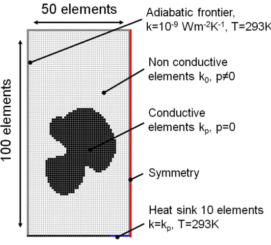
The sketch of a typical area-to-point heat conduction problem to be solved by GA is given in Figure 1. The entire domain was discretized into small and homogeneous square elements, each element having determinate conductivity, uniform temperature and heating rate. In this study, a mesh of 100×50 square elements was used, considering a compromise between calculation time and precision. Other mesh resolutions (12×25, 25×50 and 100×200) were also assessed and the effects of mesh resolution on the complexity of optimal conductive trees will be discussed in the later section.
Figure 1: geometry and mesh used for this study. Note the symmetry on the right border. Five kind of elements are defined to cover the entire calculation domain, as described below.
• Heat sink elements (blue): cells with a constant temperature (Tsink=293K) and a
thermal conductivity equal to kp. The isothermal heat sink has an aperture width of
20% of one side of the domain.
• Symmetry elements (red): the right boundary of the domain shown in Figure 1 is defined as symmetry to represent a square domain. Numerically, these elements are coded similar to adiabatic elements (quasi-perfect insulators).
• Adiabatic elements (grey): cells defined with a constant temperature (Tsink=293K, in
conductivity (typically kad/k0=10-9). The adiabatic elements and the heat sink elements
enclose the entire domain. We have verified that the kad/k0 ratio used do not influence
the estimation of temperature of the calculation domain (no thermal leaks at the borders).
• Heat generating elements (white): heat generating cells with heat generation rate p and relatively low conductivity k0.
• Conductive elements (black): cells with relatively high conductivity kp and zero heat
generation rate (p=0). The filling ratio ϕ is defined as the ratio between the number of conductive elements and the sum of conductive and heat generating elements.
Calculation domain is enclosed by symmetry, adiabatic or heat sink elements. The heat equation for conduction is solved. The domain is considered as solid and no other thermal resistances than the conduction between elements is considered.
2.2. GA procedure
The general principle of GA is to assess the best configurations among a starting random population of configurations, keep the best (those meeting best the objective function or fitness), and then cross and mutate them to get a new child population of the same size, and so on. The main procedure of GA for the area-to-point heat conduction problem is described below.
• Step 1: generate 1000 configurations with random paving of conductive and heat-generating elements with fixed ϕ and kp/k0 ratio;
• Step 3: keep the best (in terms of fitness) 200 of 1000 evaluated configurations (future parents); eliminate the others from reproduction.
• Step 4: keep the best parent as the first individual of the children population (elitism); • Step 5: cross two random parents among the best (with uniform probability) with a
random crossing probability between 0 and 20% to give two children; see next paragraph for the chromosome format.
• Step 6: mutate the two children with a random mutation probability between 0 and a maximal value for each element (see next paragraph). Correct the children so that ϕ remains constant by random substitutions;
• Step 7: go to step 5 until 1000 children are made;
• Step 8: go to step 2 until the relative residuals in temperature reach 10-6 or less for at
least 1000 iterations or no better children are found for 1000 iterations.
We introduced only three constraints in our modeling. The first constraint used is keeping the
ϕ parameter constant from one iteration to the next, which is ensured by a small sub-routine of
random balancing of elements type into the mutation function - which is not conservative by essence - in step 6. This means that the fraction of each element is forced constant after mutation to restore the balance of element types. The second constraint use is the avoidance of single (non connected to similar elements in terms of property) elements: a mutated element must have a property similar to one of its neighboring element. This fastens the convergence of shapes and still allows non connected islands of more than one isolated element to appear and survive. Finally the heat sink, symmetry and adiabatic elements are not allowed to move or mutate to keep the boundary conditions constant.
The maximal mutation probability is first initialized at 5% (first iteration), then exponentially decreased each iteration so that it is divided by two every 700 iterations. Indeed, it was found by trial and error tests that this rate allows to maximize the probability of finding better children at each iteration and consequently to speed up the convergence without "freezing" the topology into local minima.
The algorithm is stopped when the relative tolerance on temperature between two consecutive best children stays below 10-6 for 1000 iterations or if not better children are found for 1000
iterations (near convergence, each iteration or generation does not give “birth” to better configuration or children). It should be noted that the cross-over function is written to choose a random crossing direction (horizontal or vertical on each configuration) each time it is called, in order to avoid any crossing direction artifact. The "chromosome" used for crossing and mutation is just a vector of 5000 variables (50×100), each variable being an integer coding the type of elements for each element of the domain.
2.3. Calculation of the temperature field
One important step in the algorithm is the fast calculation of temperature field in the studied domain. This involves the solving of heat transfer equation numerically by a finite difference method. Details of the finite difference method for the calculation of temperature field may be referred to our earlier papers (Boichot et al. 2009; Boichot and Luo 2010) and will not be repeated here. The linear system obtained with finite difference method is solved with numerical methods optimized for sparse diagonal-dominant matrices and parallel computing and implemented with Matlab Software. Comparison with finite volume method will be given in the "Results and analysis section".
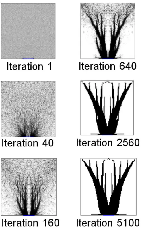
Figure 2 shows an example of topology convergence with iteration number for ϕ=0.3 and
kp/k0=10, with the objective function defined as the minimization of the peak temperature of
the domain. In this figure, the average image of 1000 conductive trees (full population at a given iteration or time) is represented versus generation number (or iteration). It can be observed that after a relatively rapid establishment of the structure frame (tree trunk) the solution converges slowly at smaller scales (branches). Using an Intel Xeon 3.60 GHz (4 processors used in parallel), a converged solution (in terms of convergence criterion chosen for a 50x100 elements domain) can be obtained within 72 hours. Each generation (iteration) costs 30 to 40 seconds calculation time (fitness evaluation + GA procedure for 1000 topologies).
Figure 2: example of topology convergence for ϕ=0.3 and kp/k0=10 vs. generation (iteration). The conductive
matter is black, the non conductive matter white. Grey levels indicate the cohabitation of several types of elements at a given position in the population for a given iteration.
3. Results and analysis
In this section, the results of GA for area-to-point heat conduction problem will be presented and analyzed. Two objective functions are identified for the study: the peak temperature and the mean temperature, with different values of ϕ and kp/k0 values. The minimization of both
objective functions will lead to the generation of conductive tree configurations.
We first performed the GA to minimize the peak temperature, then the mean temperature of the domain. The performance of the evolved configuration was assessed by the non-dimensional thermal resistances R (Bejan 1997) or A (Marck 2012) in the case of peak temperature minimization and mean temperature minimization, respectively. The two parameters are expressed as:
max sink 0 / T T R pLH k − = (1) mean sink 0 / T T A pLH k − = (2)
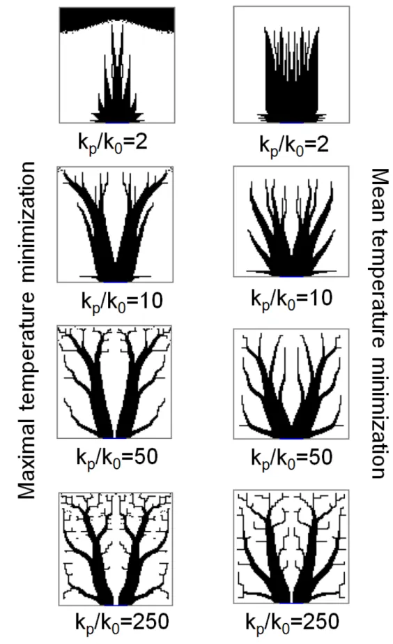
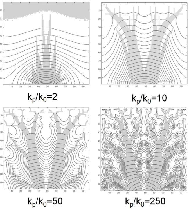
Figure 3 presents the optimal configuration of conductive path proposed by GA for peak and mean temperature minimization (ϕ=0.3; kp/k0 varying from 2 to 250). Figure 4 presents the
Figure 3: Optimal configuration proposed by GA for peak (left) or mean (right) temperature minimization (ϕ=0.3; kp/k0 from 2 to 250).
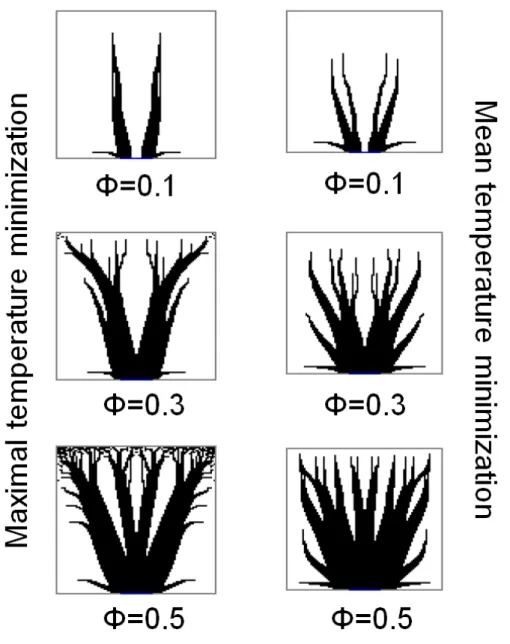
Figure 4: Optimal configuration proposed by GA for peak (left) or mean (right) temperature minimization (kp/k0=10; ϕ from 0.1 to 0.5).
From Figure 3, we may observe that similar optimal configurations (ramified trees) are obtained for two different objective functions, with the exception for kp/k0=2. For mean
temperature minimization (kp/k0=2), the optimal conductive path consists in the agglomeration
of high conductivity material around the heat sink: the heat generating elements are pushed far against the heat sink. Whereas for peak temperature minimization (kp/k0=2), a part of the
continuous cooling trees. This obviously counter-intuitive result is due to the fact that peak temperature usually appears in the farthest corners of the domain where the conductive trees try to grow toward. In case that the conductivity heat generating elements is close to that of conductive material (e.g. kp/k0=2), the conductive material will be optimally used for
reshaping the heating area. This trend is also reported by Mathieu-Potvin and Gosselin
(2007).
Figure 3 indicates the influences of conductivity ratio on the optimal configuration of conductive path, for both objective functions. Lower kp/k0 values imply thicker trunk for
draining the heat current. In contrast, higher kp/k0 values lead to slenderer trunks and more
branching levels. The high conductivity material tends to disperse through the calculation domain. Figure 4 illustrates the influence of filling ratio on the optimal configuration of conductive path. It can be observed that the higher the φ values, the thicker the trunks for a same kp/k0 ratio. It is worth noting that trees evolved based on local attraction parameters (CA
algorithms) or evolutionary algorithms (GA method) present similar trends on branching properties with respect to the kp/k0 and ϕ parameters (Boichot et al. 2009) despite the absence
of objective function in CA algorithms (local attraction).
By comparing the left column and right column on figures 3 and 4 for the same values of kp/k0
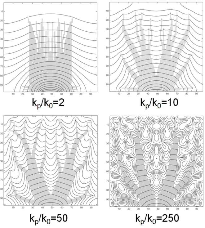
and φ, one may observe that the optimal conductive trees proposed by minimizing peak temperature are generally slenderer than those proposed by minimizing mean temperature. The conductive trees tend to cover the farthest zones from the heat sink on the domain, which consequently leads to the thermal resistance equipartition from the adiabatic boundaries to the heat sink. This may be observed by examining the temperature isolines for converged solution shown in Figures 5 and 6 (particularly figure 5).
Figure 5: temperature isolines into the geometry converged for maximal (peak) temperature minimization with ϕ=0.3 and kp/k0 from 2 to 250.
Figure 6: temperature isolines into the geometry converged for mean temperature minimization with ϕ=0.3 and kp/k0 from 2 to 250.
It appears that in case of peak temperature minimization, the GA proposes optimal conductive tree that tends to equalize as possible the temperature at the adiabatic borders, in particular for high kp/k0 ratios. This point is of particular interest: to decrease at most the peak temperature of
borders with a conductive tree. The reductio ad absurdum is to consider that if it is not the case (temperature equipartition not reached), you will always be able to lower the maximal temperature point by modifying the conductive tree in exchange of an increase of the temperature in another area of the border (which is not the hottest). We can observe in figure 5 that the higher the kp to k0 ratio, the closer to this optimal property the converged shape
tends to. There must be a particular condition in minimal kp/k0 or (kp/k0)φ that allows borders
temperature equipartition by sufficient bending of thermal streamlines.
On other hand, the isolines of figure 6 for the case of mean temperature minimization clearly indicate that such an optimality criterion is not relevant for tree evaluation.
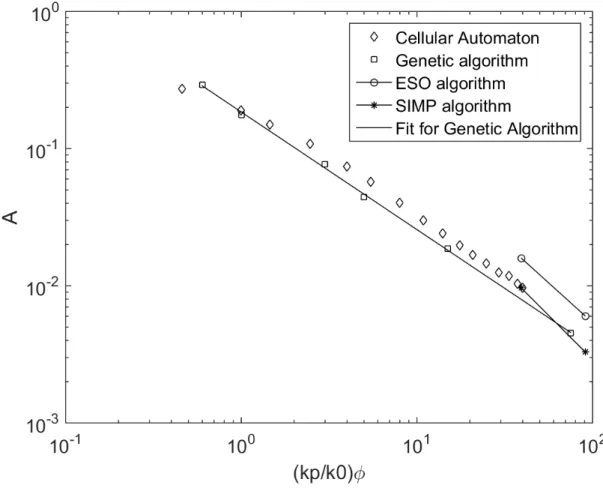
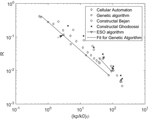
The performance of GA optimized conductive trees, measured by the non-dimensional thermal resistance R (peak temperature minimization) and A (mean temperature minimization) for different values of (kp/k0)φ product can be compared with some other numerical methods
to assess the efficiency of genetic algorithm to solve the area-to-point problem in square configuration. The A and R relationship with (kp/k0)φ for our genetic algorithm can be fitted
by the following relationships:
Figure 7 and 8 present the comparison of A and R parameters between Cellular Automaton method (CA) proposed by Boichot et al. (2009; 2010) and improved by Marck (2012), Constructal approach proposed by Bejan (1997) and modified by Ghodoossi and Egrican (2003), Evolutionary Structural Optimization (ESO) by extension proposed by Marck (2012) and SIMP model with an aggregated objective function approach (AOF) developped by Marck et al. (2012), data compiled and proposed by Marck (2012).
(
)
(
)
0.8428 0 0.8572 00.2800
/
(3)
0.1849
/
(4)
p pR
k k
A
k k
φ
φ
− −=
=
Figure 8: Benchmark of different optimization methods for R parameter. Black arrow indicates performance of trees represented in figures 11 and 12.
It appears that GA algorithm performance overcomes both constructal approach, CA and ESO algorithms. Results with SIMP algorithm are similar in terms of performance for A parameter (data not available for R parameter). It can be emphasized that GA algorithm and SIMP algorithm should be close to the optimal method to solve the area-to-point problem. Shapes obtained are interestingly very similar between GA and SIMP method also. It should be finally noted that Cellular Automaton algorithm, which is not an optimization technique per
se, can provide interesting trees, close to the GA algorithm, with a much reduced
computational effort (CA algorithm converges 3.104 faster than GA algorithm on the same
To assess whether the numerical method used in this study to calculate the temperature map (direct finite difference method) introduces a bias, we have performed cross validations with a finite volume method implemented into a commercial CFD software (CFD-Ace version 2014.0.0.11217 from ESI group), with the two converged trees obtained with the highest kp/k0
ratio (250).
Figure 9 present the comparison between Matlab temperature map calculated with direct finite difference method (5000 elements) and CFD-Ace temperature map obtained with 68772 elements (unstructured meshing), an external adiabatic frontier and nodes frontier coinciding with frontier between low and high conductivity materials for the shape converged that minimizes maximal temperature. The relative difference for R parameter is 6.3% (Matlab code slightly overestimates R compared to CFD-Ace), while the thermal isolines nearly coincide. The calculation time is 0.019 second for direct method with 5000 elements versus more than one hour for finite volume method with 68772 elements and the commercial software.
Figure 9: temperature map obtained with Matlab and CFD-Ace softwares for the shape obtained with ϕ=0.3 and kp/k0 = 250, converged for maximal (peak) temperature
minimization.
Figure 10 present the comparison between Matlab temperature map calculated with direct finite difference method (5000 elements) and CFD-Ace temperature map obtained with 64137 elements (unstructured meshing), an external adiabatic frontier and nodes frontier coinciding with frontier between low and high conductivity materials for the shape converged that minimizes mean temperature of the domain. The relative difference for A parameter is 5.6% (Matlab code slightly overestimates A compared to CFD-Ace), while the thermal isolines nearly coincide. The calculation time ratio is about the same than previously evocated.
Figure 10: temperature map obtained with Matlab and CFD-Ace for the shape obtained with ϕ=0.3 and kp/k0 = 250, converged for mean temperature minimization.
Cross validations with finite volume method implemented into a commercial software confirmed the performance of the evolved trees and indicated that the direct finite difference method used in this study tends to slightly underestimate the real physical performance of the trees converges.
Robustness analysis
In this section, a numerical benchmark is dedicated to the robustness of the GA for area-to-point heat conduction problem. More precisely, the sensitivity of mesh resolution and the reproducibility with a different random seed generator for GA are assessed, for constant values of ϕ=0.3 and kp/k0=10 and peak temperature minimization.
4.1. Mesh sensitivity
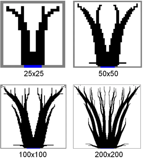
Figure 11 shows the optimal conductive trees proposed by GA, for different mesh resolutions varying from 25×25 to 200×200. The conductive tree obtained at convergence clearly depends of the mesh resolution of the domain. The coarser the mesh, the larger the smallest dimensions that will be reached by the conductive tree is. Since the configurations at convergence should barely suffer from any issue of local optimum, they can be considered as close to the best that can be expected for a given mesh resolution.
Figure 11: optimal conductive tree as a function of the mesh resolution with ϕ=0.3 and kp/k0=10.
By examining Figure 11, it is clear that the optimal solution complexity changes with the mesh resolution (and the freedom allows to algorithm), not excluding an intrinsic infinite complexity if element size tends to zero. By increasing the mesh resolution, at least at the scales performed, the converged configuration is allowed to develop slender branches and more branching levels. Each refinement of the mesh gives a refinement of the observed converged configuration. Then one question arises: is the complexity of optimal conductive
trees infinite or not? More precisely, will the branching levels always increase with increasing mesh resolution? At the still very coarse mesh resolutions we tested, it does appear that way. The solutions proposed by GA are surprisingly robust regarding different mesh resolutions, at least in the range tested. Indeed, the standard deviation of the four R values obtained fall below 0.5% for the trees presented in figure 9, and more surprisingly, the geometry 200x200 leads to the less performing tree (the best is the 100x100 elements geometry). To our point of view, this is mainly due to the poor convergence that deteriorates quality of tree for a too refined geometry: the stopping criterion of the GA algorithm is too coarse to allow the 200x200 elements geometry to converge adequately (i.e. the change of few elements should modify the objective function below the convergence criterion). The convergence for 200x200 elements geometry took 17 days, so a parametric study of stopping criterion in this particular case is currently out of reach. Additionally, the values of R parameters for trees of figure 11 are represented on figure 8: the mark size does not allow seeing any difference in value. Each tree converged is optimal at the mesh size used, which is a strong constraint by itself. It should be however noticed than with such coarse mesh as 25x25 geometry, a bias between mathematical and physical thermal performance may exist.
4.2. Reproducibility
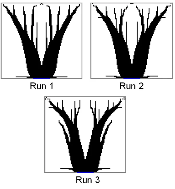
Another aspect of the robustness study is whether the configuration obtained at convergence is reproducible. In fact, a diversified configuration may possibly be obtained each time by running the GA with a different seed generator (with a Mersenne twister algorithm generating random numbers), as shown in Figure 12. It can be clearly observed that the solution converges to globally similar but locally slightly different configurations. However, the three final conductive trees have almost the same cooling effectiveness, measured by a standard
deviation on R values that falls below 0.6%. As a result, these solutions may be considered as very close to the global optimum.
Figure 12: Conductive trees at convergence with different seed generators for the random number algorithm with ϕ=0.3 and kp/k0=10.
This observation may also lead us to retrospectively consider that the differences in R values obtained by refining the mesh must be considered with caution. If the converged configurations having slight differences in local details present very close cooling performances, it means that the objective function is very flat regarding to variation of its 5000 discrete parameters near the
global optimal point. Then the open question is: is there any interest of pushing the convergence limit further for the purpose of designing real objects of practical use for thermal engineering? From the engineering point of view, once the conductive trees of a given GA iteration "condensates" (see for example in Figure 2) to a configuration with sharp borders, the further small adjustment of local details, very time consuming due to GA nature, may not noticeably augment the performance. In that sense, relaxing the convergence criterion could be a way of decreasing time needed for acceptable convergence.
From an industrial point of view, making efficient conductive tree shapes for practical use as heat sink could be easily achieved by micro fabrication, printing, laser/water cutting or metal extrusion. The issue is not how to make these objects, but what to do with these and where they can be efficiently included to improve thermal performances of real objects. This kind of fins minimizing space occupied and conductive mass could be embedded into sorption cooler beds, high temperature fuel cells (as interconnect), nuclear fuel claddings or high power electronics to decrease their thermal resistance, for example. Where thermal gradients impede the lifetime/function of objects, topology optimization could play a key role. Preliminary applications of GA algorithm applied to topology optimization to circular area-to-point problem (Luo, 2013) showed that this method is very easily expendable to any geometry without any particular code modification and even produce counter intuitive optimal solutions.
5. Conclusion
We proposed here a genetic algorithm to solve the general area-to-point heat conduction problem. Conductive trees may be generated by GA for minimizing the peak or mean temperature of the domain. Their configurations depend strongly on the values of conductivity ratio as well as the filling ratio. A robustness study on the mesh sensitivity and the reproducibility also implies that the converged solutions proposed by GA approach the
close-to-optimal configuration because of the absence of constraints used (except the square meshing of the domain) and the relative tolerance to local minima.
The main advantage of GA numerical method is clearly neither its velocity of convergence nor the easiness to define a stopping criterion, but the noticeable simplicity and more morphologic freedom offered for addressing unspecified problems. Further works should focus on numerical methods which allow fast temperature map calculation without any bias to verify if the absolute accuracy of temperature map has an influence on the evolved trees.
Acknowledgement
The authors want to thank Johan Marigny and Gaëtan Patry, students of Grenoble Institute of Technology (France), for their great contribution to the writing and debugging of the GA algorithm.
References
Bejan A. Constructal-theory network of conducting paths for cooling a heat generating volume. International Journal of Heat and Mass Transfer, 40(4):799–811, 1997.
Bejan A. (2000) Shape and structure, from engineering to nature. Cambridge University Press.
Bejan A., Lorente S. (2008) Design with constructal theory. Wiley, Hoboken.
Boichot R., Luo L., and Fan Y. Tree-network structure generation for heat conduction by cellular automaton. Energy Conversion and Management, 50(2):376–386, 2009.
Boichot R., Luo L. A simple Cellular Automaton algorithm to optimize heat transfer in complex configurations. Int. J. of Exergy, 2010 Vol.7, No.1, pp.51 – 64.
Burger F., Dirker J., Meyer J. P. (2013), Three-dimensional conductive heat transfer topology optimisation in a cubic domain for the volume-to-surface problem, International Journal of Heat and Mass Transfer, 67, 214-224.
Chen L. (2012) Progress in study on constructal theory and its applications. Sci China Ser E: Technol Sci 55:802–820.
Darwin Charles, The Origin of Species (1873). Sixth Edition, London, John Murray, Albemarle Street.
Dirker J. and Meyer J. P. (2013) Topology Optimization for an Internal Heat-Conduction Cooling Scheme in a Square Domain for High Heat Flux Applications. Journal of Heat Transfer, 135, 111010.
Errera M. R., Bejan A. Deterministic tree network for river drainage basins. Fractals, Vol. 6, 1998, pp. 245-261.
Cheng X., Li Z., Guo Z. (2003) Constructs of highly effective heat transport paths by bionic optimization. Sci China Ser E: Technol Sci 46:296–302.
Ghodoossi L. and Egrican N. Exact solution for cooling of electronics using constructal theory. Journal of Applied Physics, 93(8):4922–4929, 2003.
Goldberg David E. (1989). Genetic Algorithms in Search, Optimization, and Machine Learning. Addison Wesley, edition 1.
Gosselin L., Tye-Gingras M., Mathieu-Potvin F. (2009) Review of utilization of genetic algorithms in heat transfer problems. International Journal of Heat and Mass Transfer 52:2169–2188.
Luo L. Heat and Mass Transfer Intensification and Shape Optimization: A Multi-scale Approach (2013). Springer-Verlag London, ISBN 978-1-4471-4741-1.
Mathieu-Potvin F. and Gosselin L. Optimal conduction pathways for cooling a heat-generating. body: A comparison exercise. International Journal of Heat and Mass Transfer, 50(15- 16):2996–3006, 2007.
Marck G., Nemer M., Harion J.-L., Russeil S., et Bougeard D. Topology optimization using the SIMP method for multiobjective conductive problems. Numerical Heat Transfer, Part B: Fundamentals, 61(6):439–470, 2012.
Marck G. Thesis. Topological Optimization of Heat and Mass Transfer. Paris Institute of Technology, 2012.
Song B., Guo Z., Robustness in the volume-to-point heat conduction optimization problem, International Journal of Heat and Mass Transfer, 54, 4531-4539.
Xia Z., Cheng X., Li Z., Guo Z (2004) Bionic optimization of heat transport paths for heat conduction problems. J Enhanced Heat Transf 11:119–131.
Xu X., Liang X., Ren J. (2007) Optimization of heat conduction using combinatorial optimization algorithms. International Journal of Heat and Mass Transfer 50:1675–1682.
Zhang Y., Liu S. (2008) Design of conducting paths based on topology optimization. Heat Mass Transf 44:1217–1227.