HAL Id: hal-02456880
https://hal-imt-atlantique.archives-ouvertes.fr/hal-02456880
Submitted on 28 Jan 2020
HAL is a multi-disciplinary open access
archive for the deposit and dissemination of
sci-entific research documents, whether they are
pub-lished or not. The documents may come from
teaching and research institutions in France or
abroad, or from public or private research centers.
L’archive ouverte pluridisciplinaire HAL, est
destinée au dépôt et à la diffusion de documents
scientifiques de niveau recherche, publiés ou non,
émanant des établissements d’enseignement et de
recherche français ou étrangers, des laboratoires
publics ou privés.
Attack-tolerant Unequal Probability Sampling Methods
over Sliding Window for Distributed Streams
Yann Busnel, Yves Tillé
To cite this version:
Yann Busnel, Yves Tillé. Attack-tolerant Unequal Probability Sampling Methods over Sliding Window
for Distributed Streams. ICCDA 2020 : 4th International Conference on Compute and Data Analysis,
Mar 2020, San Jose, United States. pp.72-78, �10.1145/3388142.3388162�. �hal-02456880�
Attack-tolerant Unequal Probability Sampling Methods
over Sliding Window for Distributed Streams
Yann Busnel
Yves Till´
e
IMT Atlantique Universit´e de Neuchˆatel
IRISA, UMR CNRS 6074 Institut de statistique
Rennes, France Neuchˆatel, Switzerland
[email protected] [email protected]
January 28, 2020
Abstract
Distributed systems increasingly require the processing of large amounts of data, for metrology, safety or security pur-poses. The online processing of these large data streams requires the development of algorithms to efficiently calcu-late parameters. If elegant solutions have been proposed recently, their approximation is commonly calculated from the inception of the data stream. In a distributed execution context, it would be preferable to collect information only on the recent past (for resource saving or relevancy of most recent information). We therefore consider here the sliding window model.
In this article, we propose a family of new sampling techniques that take into account both the sliding window model and the presence of a malicious adversary. Wayne Fuller proposed in 1970 a very ingenious method of sam-pling with unequal inclusion probabilities. After doing jus-tice to this precursor paper and proposing a fast and sim-ple imsim-plementation of it, we comsim-pletely generalize Fuller’s method in order to enable the use of a tuning parameter
of spreading. The analytical results of these techniques
show the excellent performance of the generalized pivotal approach. This generalization makes the sampling method less predictable and seems appropriate to be protected from malicious attacks when sampling from a stream.
Keywords: Sampling algorithm, Sliding window, Byzan-tine adversarial, Brewer method, Pivotal method.
1
Introduction and related works
In very large distributed network management systems, it is often critical to collect global data given the very large number of participants. This can be modeled by a set of nodes, each observing a data stream. These nodes must therefore collaborate to continuously evaluate a given func-tion on the global distributed stream. For example, current network management tools analyze the input streams of a set of routers to detect malicious sources or to extract user behavior [2, 21]. The main objective is to evaluate these functions at the lowest cost in terms of space used on each node, as well as update and query time. The
prob-lem of extracting relevant information from a (distributed) data stream(s) is similar to the problem of identifying pat-terns that do not conform to the expected behaviour. This theme has been a very productive field of research in re-cent decades. For example, depending on the specificities of the domain and the type of aberrations considered, differ-ent methods have been designed: classification, grouping, nearest neighbour, spectral statistics and information the-ory. An interesting state of the art on these techniques, describing their advantages and disadvantages, is proposed by [10]. A common feature of these techniques is their high complexity in terms of space and computation cost, as they are based on algorithms with open memory, which require complete knowledge and access to the analyzed data.
Relying on algorithms of this type is not feasible in a context of real-time information extraction, with very low storage and processing capacity. However, two main ap-proaches exist for real-time processing of massive, poten-tially distributed data streams.
The first approach is to process all the data in the stream on the fly, and to keep only summaries, or aggregates, lo-cally, in which only essential information about the data is kept [10]. This approach extracts statistics on processed data streams, with bounded error probabilities, without as-suming any constraint on the order in which the data is received on the nodes (i.e., the data order could be ma-nipulated by an omnipotent opponent [4]). Most existing research using this approach has focused on calculating sta-tistical functions or measurements with a given ε error, us-ing a poly-logarithmic memory amount in the size of the stream and domain of the incoming data. These functions estimate, for example, the number of distinct data present in a given stream [23], frequency moments [1], the most fre-quent elements [11, 28], entropy of a stream [9], flood attack detection [30], the correlation between several streams [3] or the relative entropy between a biased stream and a uni-form stream [2, 5]. Unfortunately, these estimates are based on summaries that involve a significant loss of information, with sometimes drastic overestimation (as in the case of the Count-Min Sketch [14]).
On the other hand, the second consists in regularly sam-pling the stream, making it possible to limit the amount of data stored in memory [1, 24, 25, 26]. This method allows
to calculate exactly functions on these samples. However, the reliability of this calculation, in comparison with the ex-act result calculated on the entire stream, depends strongly on the volume of data that has been sampled, and the po-sition of this data on the stream. Worse still, an opponent could easily take advantage of the sampling policy to hide his attacks among the unsampled packets, or thereby pre-vent his “malicious” packets from being correlated. The primary objective of this article is to further take these two characteristics into account by using methods from survey theory.
In addition, the majority of current solutions offer
sam-pling methods over the entire stream. The use of these
techniques, for example in network monitoring, requires the selection of samples from recent data only. Carrying the well-known sampling solutions in a sliding window is often complex or even impossible given the very nature of the sampling process. In addition, classical methods do not necessarily take into account the dispersion of the sampled elements in the current window. Indeed, without stratifi-cation, the samples can be spread too evenly, or conversely concentrated in certain parts of the input stream. Adver-saries could take advantage of this knowledge to place their samples in such a way as to bias the overall sampling. The emergence of the pivotal method in survey theory suggests a relevant solution to these problems.
In a manuscript paper written in French, Deville [17] pro-posed an unequal probability sampling method that we refer to as the “Deville systematic method”. The method is also
described in detail in Till´e [31, pp. 128-130]. Another
un-equal probability sampling procedure is the pivotal method
proposed by Deville and Till´e [18] in the framework of the
splitting method [see also 31, pp. 106–08]. When the piv-otal method is applied according to the order of the units, it is usually called “sequential pivotal method” or “ordered pivotal method”. In a relatively technical paper, Chauvet [12] showed that the ordered pivotal method and Deville’s systematic method are two algorithms that implement the same sampling design, which is certainly not obvious when comparing the two methods.
Fuller [20] proposed a method where one unit is sampled in each stratum but with random strata boundaries. The method is developed for equal and unequal probability sam-pling. Fuller’s method is no other than Deville’s Systematic method with random strata boundaries.
2
Contributions and plan of the
pa-per
Our main contributions are the following. We first pro-pose a very simple implementation of Fuller’s method by means of the pivotal method. Next we generalize the piv-otal and the Fuller methods. A tuning parameter is in-troduced that enables to choose the spreading of the sam-ple. A large family of methods is then defined for the cases where the variable of interest is autocorrelated. In brief, these methods make it possible to achieve the objectives of well-spread sampling, with computational complexity and
minimal memory cost, while respecting the constraints of the aforementioned model.
In addition, to be able to theoretically study the impact of opponents on the algorithms proposed in the literature, it is possible to use different models from the distributed sys-tems community. For example, as Anceaume et al. in [7], we consider the presence of an opponent adaptive, who tries to avoid the smooth running of the algorithm by distribut-ing his data judiciously among the different streams. It is thus able to insert as much information as necessary to in-crease or reduce the accuracy of an algorithm, in relation to the current state of the system, or to reorder the streams as it sees fit. However, generally, it is considered that any algorithm run by any correct node is public knowledge to avoid some kind of security by obscurity.
3
System model
We consider a set S of ` nodes S1, . . . , S` such that each
node Si receives a large sequence σSi of data items or
units. We assume that streams σS1, . . . , σS` do not
nec-essarily have the same size, i.e., some of the items present in one stream do not necessarily appear in others or their occurrence number may differ from one stream to another
one. We also suppose that node Si (1 ≤ i ≤ `) does not
know the length of its input stream. Items arrive regularly and quickly, and due to memory constraints (i.e., nodes can locally store only a small amount of information with respect to the size of their input stream and perform simple operations on them), need to be processed sequentially and in an online manner. Nodes cannot communicate among each other. On the other hand, there exists a specific node, called the coordinator in the following, with which each node may communicate [15]. We assume that communica-tion is instantaneous. We refer the reader to [29] for a de-tailed description of data streaming models and algorithms. Note that in the some contexts such as IoT or edge com-puting, it may not be reasonable to rely on a central entity. We could extend our distributed solution to a fully decen-tralized version by organizing sites in such a way that each one could locally aggregate the information provided by its neighbours, as done in [6].
4
The pivotal method
Let’s consider a U population of size N , representing all the information that can be exchanged within the S network, in which we want to select a sample of fixed size n with
unequal inclusion probabilities 0 < πk < 1, k ∈ U, such
thatP
k∈Uπk = n. The pivotal method is particularly
sim-ple and consists of picking at each step two units (denoted by i and j) in the population. Their inclusion
probabili-ties (πi, πj) are randomly transformed to (πei,πej) using the
following randomization: (πei,πej) = (min(1, πi+ πj), max(πi+ πj− 1, 0)) with probability q (min(πi+ πj, 1), max(0, πi+ πj− 1)) with probability 1 − q,
with
q = min(1, πi+ πj) − πj
2 min(1, πi+ πj) − πi− πj
.
The validity of the method is based upon the fact that the expectation of this pair corresponds to the inclusion
prob-abilities, i.e., E(πei,eπj) = (πi, πj) and πei+eπj = πi+ πj.
This ensures that the inclusion probabilities are satisfied and that the sum of the components of the vector is always equal to n.
This elementary step can be repeated on couples of units containing values that are not equal to 0 or 1. Since at each step, a component is set to 0 or 1, in N − 1 steps at most, the sample is selected. The ordered pivotal method simply consists in taking the units according to their order in the vector of inclusion probabilities, which is built on the fly according to the incoming stream. So the first step is applied on units (1, 2). The unit that conserves a non-integer value is then confronted to unit 3 and so on.
If the sum of the inclusion probabilities is not an integer, the pivotal method ends up with a vector whose compo-nents are all integer except for one that is equal to the frac-tional part of the sum of the inclusion probabilities. This result is given for instance by the UPpivotal function of the R sampling package, which was proposed by the au-thors [27]. The pivotal method is a particular case of the cube method [19] with only one balancing variable that is equal to the inclusion probabilities. The ordered pivotal method is the particular case of the fast implementation of
the cube method proposed by Chauvet and Till´e [13].
5
Implementation
of
Fuller’s
method
In Fuller’s method as in Deville’s systematic method, the main ideas consist of constructing strata and selecting one unit in each stratum. The main problem is that it is al-most always impossible to construct strata in which the sums of the inclusion probabilities are equal to 1. In Dev-ille’s method, one first computes the cumulated inclusion probabilities Vk = k X i=1 πk with V0= 0, and VN = n.
The strata are the intervals [0, 1], [1, 2], . . . [n − 1, n]. A unit
k, such that the interval [Vk−1, Vk] contains an integer, is
called a boundary unit, because it belongs to two
consec-utive strata. The main difficulty of Deville’s systematic
method consists of avoiding selecting twice the boundary units. Drawing probabilities must be recomputed in each stratum in function of the selection in the previous stratum. The algorithm and the procedure of updating the drawing
probabilities are described in detail in Till´e [31, p.130].
Fuller’s method is exactly the same as Deville’s system-atic sampling except for the computation of the bounds of the strata. In Deville systematic sampling, the bounds are the integer numbers 0, 1, 2, . . . , n. In Fuller’s method,
1 l i b r a r y ( sampling ) 2 UPfuller<−function ( pi ,EPS= 0 . 0 0 0 0 0 0 0 1 ) 3 { 4 u=r u n i f ( 1 ) ; 5 s=UPpivotal ( c ( u , pi ) ) ; 6 s [ which ( abs ( s−u)<EPS) ] = s [ 1 ] ;
7 s [ − 1 ]
8 }
Listing 1: Implementation of Fuller’s method
the first bound is randomly selected using a uniform ran-dom variable u in [0,1]. The bounds of the strata are thus 0, u, u + 1, u + 2, . . . , n − 1 + u, n. Fuller’s method has one more stratum, but the algorithm begins by deciding ran-domly if a unit is selected in stratum [0, u] or in [n−1+u, n], which is equivalent to considering that these two intervals form a single stratum.
Chauvet [12] showed that Deville’s systematic method and the ordered pivotal method exactly implement the sam-ple sampling design. Fuller’s method can also be imsam-ple- imple-mented by the pivotal method provided that a random start is used (cf. Listing 1). Suppose that we have a vector of in-clusion probabilities which sum up to an integer. First we randomly create a phantom unit whose inclusion
probabil-ity π0 is a uniform random variable in [0,1] (line 3). Next
the ordered pivotal method is applied on this population of size N + 1 (line 4). Since the sum of the inclusion
probabil-ities is equal to n + π0, the random pivotal method returns
a vector whose components are all equal to 0 or 1 except
for one (denoted by j) that is equal to π0. Finally, unit
j is selected if the phantom unit has been selected and is not selected otherwise. The phantom unit is then removed from the sample. If the phantom unit remains with the non-integer value, it is simply removed from the sample. The code of Listing 1 gives the R implementation that is particularly simple.
6
Generalization of the Pivotal
and Fuller’s method
6.1
Main idea
The pivotal method and the Fuller method can be gener-alized. In place of confronting two units, one can consider three or more units. Suppose that r consecutive units are considered at each step. These units can be randomly trans-formed in such a way that one of them is transtrans-formed into a 0 or a 1. This transformation can be done by several pro-cedure. We propose three possible methods to transform the subsets.
6.2
Brewer’s method
Brewer [8] proposed a very interesting unequal probability
method. Till´e [31, pp. 112-114] reformulate the method as
a particular case of the splitting method. For the general-ization of the pivotal method, the method must be extended
1 brewer<−function ( pi ) 2 { 3 N=length ( pi ) ; n=sum( pi ) ; 4 a=pi∗(n−pi ) / (min(1 ,n)−pi ) ;
5 i=which ( (cumsum( a/sum( a)) − r u n i f (1)) >0 ) [ 1 ] ;
6 pim=pi∗(n−min( 1 ,n ) ) / ( n−pi [ i ] ) ;
7 pim [ i ]=min ( 1 , n ) ; 8 pim 9 }
Listing 2: Implementation of Brewer’s method
to the case where the sum of the inclusion probabilities is non-integer.
The basic step of the Brewer method can be expressed as follows:
• Select an integer number (say `) between 1 and N with probabilities (cf. lines 4 and 5 of Listing 2):
αj= X i∈U πi(n − πi) min(1, n) − πi !−1 πj(n − πj) min(1, n) − πj , j ∈ U.
• Change the vector of inclusion probabilities, for all k ∈ U , into (cf. lines 6 and 7 of Listing 2):
π`k= πk(n − min(n, 1)) n − π` if k 6= ` min(n, 1) if k = `.
The method is valid because 0 ≤ π`
k ≤ 1 for all ` ∈ U, k ∈ U, X k∈U π`k= n, ` ∈ U, and X `∈U α`π`k= πk, k ∈ U.
The short R code of Listing 2 gives an implementation. Brewer’s method has however a drawback when it is used
to generalize the pivotal method. When n =P
k∈Uπk < 1,
then all the π`
k are null except one that is equal to n. There
are then null joint inclusion probabilities. For this reason we propose to use the complementary Brewer method.
6.3
Complementary Brewer method
A complementary sampling design pc(s) of a sampling
de-sign p(s) is defined as follows:
pc(s) = p(U \s), s ⊂ U.
The complementary of the Brewer method can be derived directly from the previous section. The basic step of the complementary Brewer method will thus transform one component in a zero at each step.
• Select an integer number (say `) between 1 and N with probabilities (cf. lines 4 and 5 of Listing 3):
αj= X i∈U (1 − πi)(N − n − 1 + πi) min(1, N − n) − 1 + πi !−1 ×(1 − πj)(N − n − 1 + πj) min(1, N − n) − 1 + πj , j ∈ U. 1 complementary . brewer<−function ( pi ) 2 { 3 N=length ( pi ) ; n=sum( pi ) ; 4 a=(1−pi )∗ (N−n−1+pi ) / (min( 1 ,N−n) −1+pi ) ;
5 i=which ( (cumsum( a/sum( a)) − r u n i f (1)) >0 ) [ 1 ] ;
6 pim=1−(1−pi )∗ (N−n−min( 1 ,N−n ) ) / (N−n−(1−pi [ i ] ) ) ;
7 pim [ i ]=1−min ( 1 ,N−n ) ; 8 pim 9 }
Listing 3: Implementation of Complementary Brewer’s
method
• Change the vector of inclusion probabilities into (cf. lines 6 and 7 of Listing 2):
π`k= 1 −(1 − πk)(N − n − min(N − n, 1)) N − n − 1 + π` if k 6= ` 1 − min(1, N − n) if k = `, for all k ∈ U.
Again, the method is valid because
0 ≤ πk`≤ 1 for all ` ∈ U, k ∈ U, X k∈U πk` = n, ` ∈ U, and X `∈U α`π`k= πk, k ∈ U.
The short R code of Listing 3 gives an implementation.
6.4
Random direction method
Another method consists of generating a random vector of
size N with null mean. The code of Listing 4 gives an
implementation of this method.
For instance, N standardized random variables v1, . . . , vn
are generated and next are centered (line 4):
uk = vi− 1 N X i∈U vi.
Next, one searches the maximum value λ1and the minimum
value λ2 that satisfy
0 ≤ πk+ λ1uk ≤ 1 and 0 ≤ πk+ λ2uk≤ 1 for all k ∈ U.
This is computed between lines 5 and 7.
Finally, the vector of πk is replaced by
πknew=
(
πk+ λ1uk with probability − λ1λ−λ2 2
πk+ λ2uk with probability λ1λ−λ1 2
(cf. lines 8–11).
As in sections above, the method is also valid because
E(πnew
k ) = πk and 0 ≤ πknew≤ 1 for all k ∈ U .
6.5
General algorithm: multivotal method
and generalized Fuller method
The three methods described in the previous sections trans-form randomly one of the components of the vector into a
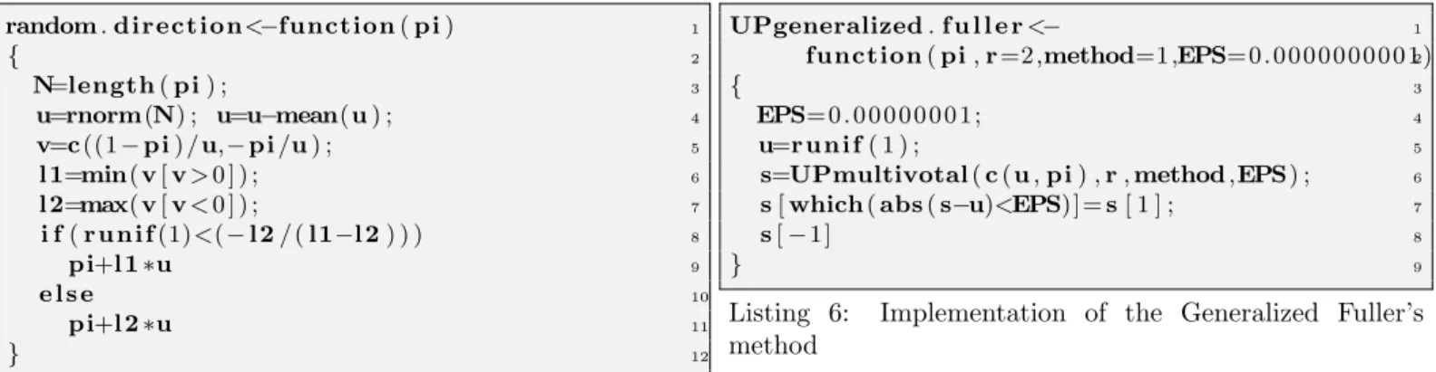
1 random . direct ion<−function ( pi )
2 { 3 N=length ( pi ) ; 4 u=rnorm(N) ; u=u−mean(u ) ; 5 v=c ((1 − pi ) / u,− pi /u ) ; 6 l 1=min( v [ v > 0 ] ) ; 7 l 2=max( v [ v < 0 ] ) ; 8 i f ( r u n i f (1)<(− l 2 / ( l1−l 2 ) ) ) 9 pi+l 1∗u 10 e l s e 11 pi+l 2∗u 12 }
Listing 4: Implementation of the Random direction method
1 UPmultivotal<−
2 function ( pi , r =2 ,method=1 ,EPS= 0 . 0 0 0 0 0 0 0 0 0 1 )
3 { 4 i f (method==1) 5 F<−function ( pi ) random . d i r e c t i o n ( pi ) 6 e l s e i f (method ==2) 7 F<−function ( pi ) brewer ( pi ) 8 e l s e 9 F<−function ( pi ) complementary . brewer ( pi )
10 a=which ( pi <(1−EPS) & pi >(0+EPS) )
11 while ( length ( a)>=r ) {
12 pi [ a [ 1 : r ] ] =F( pi [ a [ 1 : r ] ] ) ;
13 a=which ( pi <(1−EPS) & pi >(0+EPS) )
14 } 15 while ( length ( a) >1) { 16 pi [ a]=F( pi [ a ] ) ; 17 a=which ( pi <(1−EPS) & pi >(0+EPS) )
18 } 19 pi 20 }
Listing 5: Implementation of the Multivotal method
0 or a 1. When these methods are applied on a vector of size 2, they are all equal to the pivotal method.
Now, the pivotal method can be generalized. At the first step, the first r ≥ 2 units are selected. On this subset of r units, one of the three methods (Brewer, Complementary Brewer or Random direction) is applied on this subset. One of the components of this subset is transformed into a 0 or a 1. Next, the units that are not integer of this subset are completed by the following units of the stream in order to constitute again a subset of r units. Again, one of the three methods is applied and so on.
Listing 5 propose an implementation of this method. Lines 4 to 9 choose the method applied. Line 10 select non integer units from the stream, then Lines 11 to 14 apply the aforementioned method to transform one unit either in 0 or 1, one after the other. Finally, when less than r units remain non integer, the chosen method finalize the tranfor-mation (lines 15–18).
Finally Fuller’s method can be generalized by using the same trick of the phantom unit used for the pivotal method. Listing 6 proposes an implementation in R language. Line 4 uses the aforementioned trick, as line 6 applies the
Multiv-1 UPgeneralized . f u l l e r <−
2 function ( pi , r =2 ,method=1 ,EPS= 0 . 0 0 0 0 0 0 0 0 0 1 )
3 { 4 EPS= 0 . 0 0 0 0 0 0 0 1 ; 5 u=r u n i f ( 1 ) ; 6 s=UPmultivotal ( c ( u , pi ) , r , method ,EPS) ;
7 s [ which ( abs ( s−u)<EPS) ] = s [ 1 ] ;
8 s [ − 1 ]
9 }
Listing 6: Implementation of the Generalized Fuller’s
method
otal method on this modified vector.
7
Simulations
In order to simulate the behavior of these methods on data streams, an artificial population of size N = 200 has been generated with heteroscedasticity and auto-correlation. First an auto-correlated variable has been
cre-ated by εk= 0.9 εk+ ukwhere ε1and uk(k = 2, . . . , N ) are
independent standardized normal random variables. Next
the xkare independent Gamma variables with shape 5, rate
= 0.25. The interest variables are yk= xk(4+εk). The
sam-ple size is set to n = 50 and the inclusion probabilities are
proportional to xk.
A set of 200,000 simulations is run to approximate the variances of the different methods. Then, to evaluate the quality of each sample provided by these methods, the
H´ajek estimators are next computed [22]:
b Y = P k∈U ykak πk P k∈U ak πk ,
where ak= 1 if k is selected in the sample and 0 otherwise.
We consider the variance of the H´ajek estimator for the
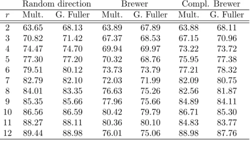
random pivotal method as the baseline of our comparisons. This variance is equal to 39.14376 (100%). The variance of the pivotal method equals 25.09 (64.07%), that is 64.07% of the variance of the random pivotal method. More inter-estingly, for the Fuller method, the variance equals 26.67 (68.13%).
Table 1 contains the ratios of variances of bY for the other
method and different values of r with respect to the ran-dom pivotal method. When r = 2, all the methods reduce to the pivotal or the Fuller method. Unsurprisingly, when r increases, the variance increases. Figure 1 illustrates the results presented in Table 1. Moreover the “Brewer” meth-ods are a little more accurate. This is probably due to the fact that the probabilities are more likely to be set to zero during the algorithm. The Brewer methods are thus more repulsive.
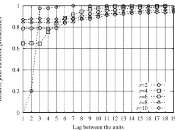
Figures 2 and 3 contain examples (with N = 20, n = 7
and equal inclusion probabilities) where πk`/(πkπ`) is
plot-ted in function of |k − `| for different values of r. This corresponds to the normalized second order probabilities (divided by the first order probabilities). The larger r, the
Table 1: Variances of the H´ajek estimators for the different sampling designs over 200,000 simulations.
Results are given for the multivotal method (Mult.) and Generalized (G.) Fuller method with the three possibilities: Random direction, Brewer, and Complementary (Comp.) Brewer method.
Random direction Brewer Compl. Brewer
r Mult. G. Fuller Mult. G. Fuller Mult. G. Fuller
2 63.65 68.13 63.89 67.89 63.88 68.11 3 70.82 71.42 67.37 68.53 67.15 70.96 4 74.47 74.70 69.94 69.97 73.22 73.72 5 77.30 77.20 70.32 68.76 75.95 77.38 6 79.51 80.12 73.73 73.79 77.21 78.32 7 82.79 82.10 72.03 71.99 82.09 80.75 8 84.01 83.35 76.63 75.26 82.56 81.87 9 85.35 85.66 77.96 75.66 84.89 84.11 10 86.56 86.59 80.42 79.79 86.71 85.30 11 88.27 88.11 80.36 80.10 84.83 83.77 12 89.44 88.98 76.01 75.06 88.98 87.76
Variance of the Hájek estimators
r
Random direction − Multivotal Random direction − Generalized Fuller Brewer − Multivotal Brewer − Generalized Fuller Complementary Brewer − Multivotal Complementary Brewer − Generalized Fuller 55 60 65 70 75 80 85 90 2 4 6 8 10 12
Figure 1: Variances of the H´ajek estimators for the different
sampling designs over 200,000 simulations.
Results are given for the multivotal method (Mult.) and Generalized (G.) Fuller method with the three possibilities: Random direction, Brewer, and Complementary (Comp.) Brewer method.
inclusion probabilities tends to a situation of independence, which is the less predictable situation. In other words, if these probabilities are constant, it means that selecting one unit does not provide information on selecting the next. This property is particularly interesting in the presence of a powerful adversary. Indeed, the latter will not be able to take advantage of the knowledge of the last sampled items to place his own malicious items knowingly.
On both figures, one can observe that when r = 2, select-ing the unit makes it very unlikely to select the next unit. When r is higher, the probabilities tend to equalize. This makes it much harder to predict what will happen next.
Relative joint inclusion probabilities
Lag between the units
r=2 r=4 r=6 r=8 r=10 0 0.2 0.4 0.6 0.8 1 1 2 3 4 5 6 7 8 9 10 11 12 13 14 15 16 17 18 19
Figure 2: Relative joint inclusion probabilities, over
1,000,000 simulations, for the Generalized Fuller method with the Complementary Brewer method
8
Discussion and extensions
Wayne Fuller has been really a precursor in the sense that he proposed a method that is more general by using ran-dom boundaries. His paper is very technical and the im-plementation can be simplified. Fuller’s method is however an excellent procedure. The sample is spread by the use of strata with random boundaries. The new implementation enables to define a fast and sequential algorithm. The joint inclusion probabilities are not null, which is an advantage with respect to the use of nonrandom boundaries. A sim-ple expression for the joint inclusion probabilities remains to be found and seems to be really challenging. The pivotal method can also be generalized by confronting more than two units at each step. This generalization makes the
sam-Relative joint inclusion probabilities
Lag between the units
r=2 r=4 r=6 r=8 r=10 0 0.2 0.4 0.6 0.8 1 1 2 3 4 5 6 7 8 9 10 11 12 13 14 15 16 17 18 19
Figure 3: Relative joint inclusion probabilities, over
1,000,000 simulations, for the Multivotal method with the Random direction method
pling method less predictable and could be appropriate to be protected from malicious attacks when sampling from a stream.
In one hand, if r equals 2 all the methods reduce to the
pivotal method. On the other hand, if r equals N , the
procedure reduces the method of Brewer, complementary Brewer or random direction. In this last case all the units are involved in the next step of the procedure. When r = 2, the next step is very predictable because the next decision will only concern two units. If r = N , nothing can predict which units will be selected from the following N . Param-eter r can be used to tune the design. The larger r, the most unpredictable is the selection of the following units. However the smaller r, the more accurate is the estimator. Between these two values a tradeoff can be find according to the considered problem.
In addition, all these algorithms allow to take into ac-count the needs of sliding windows. The sliding window model formalized by Datar et al. [16] defines the validity period of an element, i.e., the sample will only be drawn
from the more recent N0 << N elements among the U
ele-ments already observed. In this model, the samples arrive
continuously and expire after exactly the N0 steps. A step
corresponds to the arrival of an element of the population, we consider sliding windows based on counting. The chal-lenge is to perform this calculation in the sublinear space.
When N0 is set to the maximum value N , the sliding
win-dow model is reduced to the classic model. The additional problem with a sliding window is that when a prefix of a stream is summarized, we lose the time information related to the different elements, making the exclusion of the oldest elements non-trivial with little memory. The interest of the methods presented above relies in the inherent stratification of sampling. Also, it is sufficient to keep the samples taken
in the last N0 strata to make the method reliable, efficient
and robust in a sliding window.
Finally, we propose an algorithmic adaptation that al-lows sampling according to any of the techniques presented
above on a set of ` distributed data streams, so that the number of bits communicated between the ` sites and the coordinator is minimal. This amounts to the coordinator
gathering all the samples on the previous window. The
union then represents a meaningful sample of the overall distributed stream. As mentioned earlier in Section 3, it is possible to have a fully decentralized version of our algo-rithm, for example by organizing nodes within a distributed hash table (DHT) and by taking advantage of the additive property of the samples to allow each site to collect its pat-tern and gradually obtain a global view of the current sam-ple. Such a possible solution appears in [6]. It should be noted, however, that the distributed version would have a significant impact on the cost of communication. This issue is left open for future work.
References
[1] N. Alon, Y. Matias, and M. Szegedy. 1996. The space complexity of approximating the frequency moments. In Proceedings of the 28th ACM Symposium on Theory of computing (STOC). 20–29.
[2] E. Anceaume and Y. Busnel. 2014. A Distributed In-formation Divergence Estimation over Data Streams. IEEE Transaction on Parallel and Distributed System
25, 2 (2014), 478–487. https://doi.org/10.1109/
TPDS.2013.101
[3] E. Anceaume and Y. Busnel. 2017. Lightweight Metric Computation for Distributed Massive Data Streams. Transaction on Large-Scale Data- and Knowledge-Centered Systems 33 (2017), 1–39.
[4] E. Anceaume, Y. Busnel, and S. Gambs. 2010. Uni-form and Ergodic Sampling in Unstructured Peer-to-Peer Systems with Malicious Nodes. In Proceedings of the 14th International Conference on Principles of Distributed Systems (OPODIS), Vol. 6490. 64–78. https://doi.org/10.1007/978-3-642-17653-1_5 [5] E. Anceaume, Y. Busnel, and S. Gambs. 2012.
An-KLe: Detecting Attacks in Large Scale Systems via Information Divergence. In Proceedings of the 9th Eu-ropean Dependable Computing Conference (EDCC). https://doi.org/10.1109/EDCC.2012.9
[6] E. Anceaume, Y. Busnel, and N. Rivetti. 2015. Esti-mating the Frequency of Data Items in Massive Dis-tributed Streams. In Proceedings of the 4th IEEE Sym-posium on Network Cloud Computing and Applications
(NCCA). 59–66. https://doi.org/10.1109/NCCA.
2015.19
[7] E. Anceaume, Y. Busnel, N. Rivetti, and B. Seri-cola. 2015. Identifying Global Icebergs in Distributed Streams. In Proceedings of the 34th IEEE Sympo-sium on Reliable Distributed Systems (SRDS). 266– 275. https://doi.org/10.1109/SRDS.2015.19
[8] Kenneth R. W. Brewer. 1975. A simple procedure for
πpswor. Australian Journal of Statistics 17 (1975),
166–172.
[9] A. Chakrabarti, G. Cormode, and A. McGregor. 2007. A near-optimal algorithm for computing the entropy of a stream. In Proceedings of the 18th ACM-SIAM Symposium on Discrete Algorithms (SODA). 328–335. [10] V. Chandola, A. Banerjee, and V. Kumar. 2009.
Anomaly detection: A survey. Comput. Surveys 41, 3 (2009), 1–58.
[11] M. Charikar, K. Chen, and M. Farach-Colton. 2004. Finding frequent items in data streams. Elsevier The-oretical Computer Science 312, 1 (2004), 3–15. [12] Guillaume Chauvet. 2012. On a characterization of
ordered pivotal sampling. Bernoulli 18, 4 (2012), 1320– 1340.
[13] Guillaume Chauvet and Yves Till´e. 2006. A fast
algo-rithm of balanced sampling. Journal of Computational Statistics 21 (2006), 9–31.
[14] G. Cormode and S. Muthukrishnan. 2005. An
im-proved data stream summary: the count-min sketch
and its applications. Journal of Algorithms 55, 1
(2005), 58–75.
[15] G. Cormode, S. Muthukrishnan, and K. Yi. 2008. Al-gorithms for distributed functional monitoring. In Pro-ceedings of the 19th ACM-SIAM Symposium On Dis-crete Algorithms (SODA).
[16] M. Datar, A. Gionis, P. Indyk, and R. Motwani. 2002. Maintaining Stream Statistics over Sliding Windows. SIAM J. Comput. 31, 6 (2002), 1794–1813.
[17] Jean-Claude Deville. 1998. Une nouvelle (encore une!)
m´ethode de tirage `a probabilit´es in´egales. Technical
Report 9804. M´ethodologie Statistique, Insee, Paris.
[18] Jean-Claude Deville and Yves Till´e. 1998. Unequal
probability sampling without replacement through a splitting method. Biometrika 85 (1998), 89–101.
[19] Jean-Claude Deville and Yves Till´e. 2004. Efficient
balanced sampling: The cube method. Biometrika 91 (2004), 893–912.
[20] Wayne Arthur Fuller. 1970. Sampling with random stratum boundaries. Journal of the Royal Statistical Society B32 (1970), 209–226.
[21] S. Ganguly, M. Garafalakis, R. Rastogi, and K. Sab-nani. 2007. Streaming Algorithms for Robust, Real-Time Detection of DDoS Attacks. In Proceedings of the 27th International Conference on Distributed Comput-ing Systems (ICDCS ’07). IEEE Computer Society, 4.
[22] Jaroslav H´ajek. 1971. Discussion of an essay on the
logical foundations of survey sampling, part on by D. Basu. In Foundations of Statistical Inference, Vidyad-har Prabhakar Godambe and D. A. Sprott (Eds.). Holt, Rinehart, Winston, Toronto, 326.
[23] D. M. Kane, J. Nelson, and D. P. Woodruff. 2010. An Optimal Algorithm for the Distinct Element Problem. In Proceedings of the 29th ACM Symposium on Prin-ciples of Database Systems (PODS).
[24] V. Karamcheti, D. Geiger, Z. Kedem, and S.
Muthuskrishnan. 2005. Detecting malicious network traffic using inverse distribution of packet contents. In Proceedings of the 1st Workshop on Mining Network Data (MineNet).
[25] B. Krishnamurthy, S. Sen, Y. Zhang, and Y. Chen. 2003. Sketch-based Change Detection: Methods, Eval-uation, and Applications. In Proceedings of the 3rd ACM SIGCOMM Internet Measurement Conference (IMC). 234–247.
[26] A. Lakhina, M. Crovella, and C.Diot. 2005. Mining Anomalies Using Traffic Feature Distributions. In Pro-ceedings of the 28th ACM Conference on Applications, Technologies, Architectures, and Protocols for Com-puter Communications (SIGCOMM).
[27] Alina Matei and Yves Till´e. 2016. The R
sampling package, Version 2.8.
Univer-sit´e de Neuchˆatel https://cran.r-project.org/
web/packages/sampling/index.html.
[28] A. Metwally, D. Agrawal, and A. El Abbadi. 2005. Effi-cient Computation of Frequent and Top-k Elements in Data Streams. In Proceedings of the 10th International Conference on Database Theory (ICDT).
[29] S. Muthukrishnan. 2005. Data Streams: Algorithms and Applications. Now Publishers Inc.
[30] O. Salem, S. Vaton, and A. Gravey. 2010. A
scal-able, efficient and informative approach for anomaly-based intrusion detection systems: theory and prac-tice. International Journal of Network Management 20, 5 (2010), 271–293.
[31] Yves Till´e. 2006. Sampling Algorithms. Springer, New