HAL Id: hal-01347786
https://hal.archives-ouvertes.fr/hal-01347786
Submitted on 21 Jul 2016
HAL is a multi-disciplinary open access
archive for the deposit and dissemination of
sci-entific research documents, whether they are
pub-lished or not. The documents may come from
teaching and research institutions in France or
abroad, or from public or private research centers.
L’archive ouverte pluridisciplinaire HAL, est
destinée au dépôt et à la diffusion de documents
scientifiques de niveau recherche, publiés ou non,
émanant des établissements d’enseignement et de
recherche français ou étrangers, des laboratoires
publics ou privés.
Distributed under a Creative Commons Attribution| 4.0 International License
Improving clustering techniques in wireless sensor
networks using thinning process
Monique Becker, Ashish Gupta, Michel Marot, Harmeet Singh
To cite this version:
Monique Becker, Ashish Gupta, Michel Marot, Harmeet Singh. Improving clustering techniques in
wireless sensor networks using thinning process. Performance Evaluation of Computer and
Commu-nication Systems (PERFORM), Oct 2010, Vienne, Austria. pp.203-214,
�10.1007/978-3-642-25575-5_17�. �hal-01347786�
Improving Clustering Techniques in Wireless
Sensor Networks Using Thinning Process
Monique Becker, Ashish Gupta, Michel Marot, Harmeet Singh
CNRS–SAMOVAR–UMR 5157 – TELECOM SudParis ; 9 Rue Charles Fourier, 91011 EVRY, FRANCE
{Monique.Becker,Ashish.Gupta,Michel.Marot}@telecom-sudparis.eu, [email protected]
Abstract. We propose a rapid cluster formation algorithm using a thin-ning technique : rC-MHP(rapid Clustering inspired from Mat´ern Hard-Core Process). In order to prove its performance, it is compared with a well known cluster formation heuristic: Max-Min. Experimental results show that rC-MHP outperforms Max-Min in terms of messages needed to choose the cluster head, cluster head maintenance and memory require-ment, comprehensively in sparse as well as in dense networks. We show that rC-MHP has a scalable behavior and it is very easy to implement. rC-MHP can be used as an efficient clustering technique.
1
Introduction
An ideal wireless sensor node consumes very little power, is software programmable, is capable of fast data acquisition and processing and costs little to purchase and install. To preserve energy, clustering is necessary in large networks. To our best knowledge, there are experimental analysis of sensors but not of clustering. Some objectives of clustering are listed below:
– Data aggregation and updates take place in Cluster Heads(CHs). – Reduce network traffic and the contention for the channel.
– Cluster structure gives the impression of a structured and more stable net-work.
This paper proposes and validates a new clustering algorithm, rC-MHP (rapid Clustering inspired from Mat´ern Hard-Core Process). We observed from our experimental work on sensor networks (see [1], [2]) and from literature, e.g. [3], that sensor networks’ behavior appeared to be much more complex than the theory led us to expect it to be. So, we validate rC-MHP empirically. Of course, in an empirical approach we can only have a limited number of sensors. Later on, these results can be integrated in simulations for the large networks.
In stochastic geometry, (see [4] page- 145-165), “Thinning operation uses some definite rule to delete points of a basic process.” The thinning processes can be characterized into two types: independent and dependent thinning pro-cesses. In case of independent thinning, the points are independent of each other
(location, in case of sensor nodes) and vice-versa in the other case. The Mat´ern Hard-Core Process (MHP) [4] is a dependent thinning process which is usually applied to a stationary Poisson point process. Here, we apply it for choosing cluster heads in rC-MHP.
Max-Min d cluster formation [5], proposes a distributed and scalable way of forming clusters in ad hoc networks. In Max-Min, each node has a weight and, based on the weight, a node decides whether it can be a cluster head or not. The d-dominating1 set of CHs is first selected by using nodes identifiers and then
clusters are formed. It does not give an optimal solution as the problem is NP-hard but it is a well known and efficient heuristic in selecting nodes having a high criterion value. In [6] the authors further corrected, validated and generalized Max-Min heuristic and showed that the rule 2 of the cluster formation may create loops in the network. The cluster formation seems very distributed once the weights are allocated to the nodes.
This paper shows that if each node wants to know the clustering criteria for its neighbors then there is a serious implementation problem in the real world. We test and compare a well known cluster formation heuristic (Max-Min) with our proposed method(rC-MHP) and show that rC-MHP is far more suited for the sensor networks. Max-Min is theoretically distributed and thus scalable. How-ever, it is unscalable in practice because of the specific features of sensors: their limited memory. In contrast, rC-MHP behaves like a scalable algorithm. This paper shows, due to insignificant memory requirement and clustering overheads, rC-MHP outperforms Max-Min as an efficient way of clustering. These results are based on real experiments conducted on Tmote Sky sensors.
1.1 Description of the Mat´ern Hard core Process
If the characteristics of the basic process are known then it is straightforward to calculate the characteristics of the point process produced by an independent thinning (cf. [4], page- 145-165). Thus, if Φ is the result of a p(x)-thinning of Φb, then its intensity measure ∧ for a Borel set B is given by
∧(B) = Z
B
p(x)λbdx (1)
The Mat´ern Hard core Process (MHP)[4] is essentially a dependent thinning applied to a stationary Poisson Point process Φb of intensity λb. The points of
Φb are marked independently by random numbers uniformly distributed over
{0; 1}. The dependent thinning retains the point x of Φb with mark m(x) if the
sphere b(x, h) contains no point of Φb with marks smaller than m(x). Formally,
the thinning process Φ is given by:
Φ = {x ∈ Φb: m(x) < m(y)∀y ∈ Φb∩ b(x, h)\{x}} (2)
1
A d dominating set of the CHs is a set such that any node is not more than d hops away from its CH.
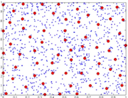
Fig. 1: Cluster-head positions after having applied the Mat´ern Hard core Poisson process where the intensity of the nodes is λ = 1000 and the distance h = 0.1 m. The side length of the square is 1 m.
The Fig. 1 shows the location of the cluster heads when the sensors are dis-tributed via a Poisson point process with intensity 1000. Here, m(x) is the coordi-nate of a node. Initially, a node is randomly selected. Then, the Mat´ern hard-core process is applied and points are selected as cluster heads. The basic principle to use rC-MHP as the clustering mechanism is that inside an area/sphere there can only be a single cluster head. If the node falls in a zone where a CH is already present, it can’t become a CH. In the real implementation, the Node id will be the mark (m(x)) and h will be the LQI.
According to Baccelli et al. [7], the Mat´ern hard core process is a natural model for the access scheme of HiPERLAN (High Performance Radio LAN) type 1 and the MAC of HiPERLAN type 1 actually uses an advanced version of CSMA. [8] suggests that the MHP distribution gives regular points.
1.2 Description of Max-Min cluster Formation Heuristic
The WSN can be modeled as a graph G = (V, E), where two nodes are connected by an edge if they can communicate with each other. Let x ∈ V be a node in the WSN. N (x) is the set of neighbors of the node x and W (x) is the weight of the node, which in our case is the degree of connectivity denoted D(x). The clusterheads form a subset S of V which is a d − dominating set over G. Let X be the image set of V by v ; v is a bijection of V over X. The reverse function is denoted v−1: ∀x ∈ V, v−1(v(x)) = x.
Max-Min uses 2d + 1 rounds, where d is the number of hops. A node can be d hops away from its CH. The algorithm includes 2d runs. The d first runs constitute the Max phase. The d last runs constitute the Min phase2. Each node
updates two lists, Winner and Sender, of 2d + 1 records. Winner is a list of
2The min is intended to avoid that a node which is too far from the max node gets
to be CH even if it has lower mark. So, the idea is that a CH may be the minimum among the max marked, and it will get the lower mark nodes.
elements of X. Sender is a list of elements of V . Let us denote Wk(x) and Sk(x)
the images of x for the functions Wk and Sk, defined by induction.
The basic idea of the d − dominating set is: in the first phase, the Max phase, a node determines its dominating node (for a given criterion) among its d hop neighbors; then, in the Min phase, a node knows whether it is a dominating node for one of its neighbor nodes. If it is the case, this node belongs to the set S. For a given criterion, the only dominating set is built from this very simple process. Initial Phase k = 0
∀y ∈ V, W0= D(x), S(x) = x (3)
FloodMax Phase: k ∈ [|1; d|]
Assuming that ∀x ∈ V , Wk−1(x) and Sk−1(x) are known in the previous step.
Let yk(x) be a unique node in N (x) defined by:
∀y ∈ N (x)\yk(x), Wk−1(yk(x)) > Wk−1(y) (4)
Wk and Sk are calculated as follows:
∀x ∈ V, Wk−1(yk(x)), Sk(x) = yk(x) (5)
FloodMin Phase: k ∈ [|d + 1; 2d|],
Assuming that ∀x ∈ V , Wk−1(x) and Sk−1(x) are known in previous step. Let
yk(x) be the unique node in N (x) defined by:
∀y ∈ N (x)\yk(x), Wk−1(yk(x)) < Wk−1(y) (6)
Wk and Sk are calculated as follows:
∀x ∈ V, Wk−1(yk(x)), Sk(x) = yk(x) (7)
The set of CHs is defined as follows:
S = {x ∈ V, W2d(x) = v(x)} (8)
2
Implementation
As per the definition of the Zigbee standard [9], the Link Quality Indication (LQI) measurement is a “characterization of the strength and/or quality of a received packet”. Therefore, we used the LQI as a channel quality indicator be-tween two nodes to create clusters. In case of the CC2420 trans-receiver, the LQI values range from 50 to 110. The minimum transmission power of the radio is -25 dBm which corresponds to a 5-6 m communication range. The maximum transmission power is 0 dBm which corresponds to 70 m (indoor). Both cluster-ing algorithms use beacons for routcluster-ing and the Base Station (BS) is their final destination. To filter out the bad links, we use a threshold LQI of 106 which corresponds to 98% Packet Reception Rate (PRR) [10]. All the nodes are in direct line of sight. We use the default CSMA/CA available in the TinyOS stack.
Fig. 2: rC-MHP
2.1 rC-MHP: a rapid Clustering inspired from MHP
rC-MHP as described in Fig. 2 is implemented in 6 steps:
Step 1: The BS declares itself as cluster head and sends beacons. When other nodes receive those beacons they check the LQI of these received beacons. If the LQI is ≥ 106, they join the BS as cluster nodes and form a cluster.
Step 2: Nodes receiving beacons from the BS with LQI < 106 declare themselves as CHs.
Step 3:A conflict may arise if more than one node in the same Mat`ern zone declare themselves as CHs.
Step 4: This conflict is resolved using the node-id. Nodes with higher Id will cease to be a CH.
Step 5: A node ceasing to be a CH sends special messages: “I am no longer a CH”.
Step 6: The other nodes receiving these special messages from their former CH participate again in the clustering process. A node waits/pauses before declaring itself to be CH to check (1) if it is still under influence of some other CH or (2) if all of its neighbors have had enough time to send the beacon. This makes clustering more efficient.
Once the clustering is over, the HybridLQI algorithm [11] is used as the inter-cluster routing algorithm. The HybridLQI improves the performance of the MultihopLQI in asymmetric wireless link sensor networks. In HybridLQI, every node maintains the number of messages it sends to each of its neighbors and how many of them are being acknowledged. In this manner, the packet loss percentage (uplink channel quality) over the links is calculated. Beacons and the LQI are used to estimate the down-link channel. Therefore, without adding any extra cost to the network, the bidirectional channel quality is calculated. The MultihopLQI obtains the link quality from the LQI calculated from the received beacon (downlink) and assumes that the bidirectional links are symmetric.
Functioning: Initially, all nodes (except the BS) are unconnected (i.e., there is no path to the BS). All clustering will be done from beacon messages which are also being used for routing. BS (default CH) starts sending beacon messages. The reception of beacons is handled via three cases:
Case 1: If a node receives a beacon message from a CH with LQI ≥ 106, three more conditions are possible:
– If the node is not connected, it will join that CH and set its status as con-nected node. Then, it starts sending beacon messages.
– If the node is connected but itself is not a CH, it will keep this CH in its cluster table.
– If it is a CH, it will check (via node id) if it can remain CH or not.
Case 2: If an unconnected node receives a beacon message from a connected node (either a cluster head or any other node which is connected), it checks if it can declare itself as clusterhead or not.
Case 3: The CHs use these beacons to discover a route towards the BS. The other nodes which are not CH will simply route to their clusterhead. Now, the CHs will send this packet to the BS. If two CHs are out of range they will communicate via a intermediate node of the other CH. A CH will never route its packets via a node which is in its cluster.
2.2 Max-Min algorithm
Fig. 3: Max-Min Algorithm
Max-Min algorithm (for d = 1) is described in Fig. 3. It is implemented in 5 phases.
1. Phase 1: Each node broadcasts its Phase 1 message with T T L = 1 (Time To Live). This is done for the neighbor discovery. As in the case of rC-MHP, to be considered as a neighbor, the LQI between two nodes should be >= 106. In this way, the nodes determine their own weight (degree of connectivity, D(x)) and store this information in the neighbor table (a single entry per neighbor).
– Max-Min’s requirement to store information for all of its neighbors is inconvenient and needs memory.
– If any node misses these phase packets, the selection of the CH may not be sound. Therefore, a node must send its Phase 1 messages repeatedly to ensure that all of its neighbors have received a phase message. The nodes which are in Phase 1 can only participate in Max-Min cluster formation heuristic.
2. Phase 2: Once a node finishes computing its weight, it needs to broadcast that weight again with T T L = 1. So, it sends the Phase 2 messages. The nodes which are in Phase 2 can only process these received phase packet (under condition LQI ≥ 106). Based on these packets, at the end of the Phase 2, each node knows the Node Id associated with the maximum weight. 3. Phase 3: The nodes send phase messages with their maximum weight as information. Accordingly, the neighbor tables are updated. This marks the end of the floodmax phase.
4. Phase 4: When the max weight is known, the nodes perform another set of calculations to know the minimum weight associated with the node and then broadcast it.
5. Phase 5: Finally, a node can decide if it can become a CH or not. A CH then sends a burst of beacon messages. On reception of these beacon messages, a non-CH node joins a cluster.
Why to pause after each phase: Initially, the nodes are switched ON at different time. So, to avoid a phase mismatch among the nodes, the nodes must wait before entering a new phase. During the pause, a node waits to receive phase messages from the other nodes, if it detects a new node then it retransmits its own phase packet.
After clustering, the HybridLQI is used for inter-cluster routing. If two CHs are out of the range they will communicate via a intermediate node of the other CH. The CH will never route its packets via a node which is in its cluster.
3
Analysis
The Table 1 lists the network deployment parameters for the rest of the pa-per. In the case of Max-Min, the term “Phase/Signal Message” refers to control messages that are used to form clusters. In case of rC-MHP, the term “Special Message” refers to control messages that are used to form/maintain clusters. A BEACON TIME OUT may be triggered if a node does not receive some beacon from its CH. A BEACON TIME OUT will lead to the eviction of the CH from the cluster/parent table of the node. However, the value of the BEA-CON TIME OUT should be sufficiently large to avoid a network instability. The cluster maintenance is also important as radio links are unreliable [1].
3.1 Effect of the node density on Max-Min
In Max-Min, the selection of CHs needs a lot of run time memory. Due to the limited available memory in the sensors, the size of the neighbor table was set
Table 1: Deployment Parameters
Packet Size 78 bytes
Frequency 6 packets per minute Beacon Frequency 2 per minute BEACON TIME OUT 4 x Number of nodes Maximum Number of retries 5
Transmission Power -25 dBm Maximum Transmission Range Possible 5-6 meters
Channel 11
Threshold LQI 106 Maximum Distance for Threshold LQI 3 meters
to 12. The effect of the node density is shown via an example. We conducted two tests: first with 12 nodes whereas the second with 30 nodes. Both of these tests were conducted over an area of 5 m × 4 m. Basically, in the second set, we increased the node density of the network. In our implementation, Max-Min can only store up to 12 nodes. Further, by choosing 30, we are testing the case when the number of immediate neighbors are around 250% of the memory capacity.
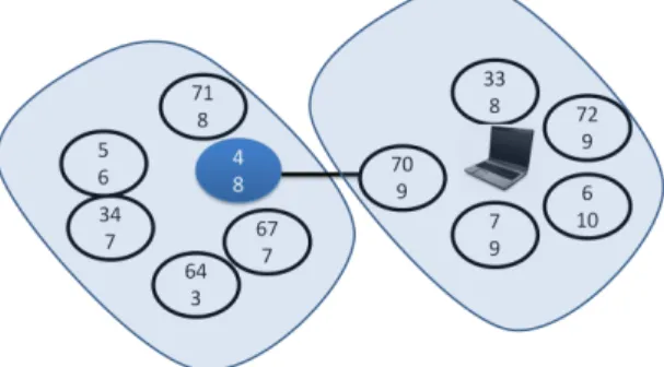
Fig. 4: Node id with its own weight. Clusters produced by Max-Min. There are 12 nodes including the BS.
Case A: 12 nodes including the BS: The Fig. 4 illustrates that Max-Min formed two clusters. In this experiment, the node 4 became a CH after comple-tion of all the phases of Max-Min. So, the node 4 sent its beacon declaring that “I am a CH”. Similarly, the BS (default CH) also sent its beacon declaring itself to be a CH. On the reception of these beacons, Non-CH nodes decided to join the respective cluster (based on first come first served basis).
Case B: 30 nodes including the BS: Fig. 5 illustrates that several clusters were produced by Max-Min when 30 nodes were deployed in the network. As the size of the neighbor was set to 12, the nodes were able to store up to 12 neighbors. We can see that most of the nodes have a weight equal to 12. What
Fig. 5: Max-Min cluster formation, 30 nodes with node id and weight
happened is, the node A was in the neighbor table of the node B but the node B was not in the neighbor table of the node A. Due to this mismatch, several nodes became CH and more nodes became singleton clusters as fewer nodes were available to join many CHs.
Due to the limited memory capacity of the sensors, the scalability of Max-Min’s is inhibited by its basic requirement: to know and store the weights of each of its neighbor. Hence, Max-Min is not scalable in practice.
3.2 Effect of the node density in rC-MHP
– rC-MHP does not need to store any clustering criteria for any of its neigh-bors. If a node is under the area of influence of a CH, it cannot declare itself as a CH. Therefore, the memory needed is independent of the node density. – In rC-MHP, if the nodes have changed their state (CH ⇔ non-CH), they need to broadcast (TTL = 1) very few packets. Sensors don’t need to know their degree of connectivity. So, a short burst of special message packets is enough in rC-MHP to diffuse changes. Underlying CSMA/CA ensures the channel availability.
– After the BEACON TIME OUT, a node will either join a CH or declare itself as a CH. Similarly, if the channel quality changed, a node may declare itself as a CH. Hence, rC-MHP will inherently do the clustering.
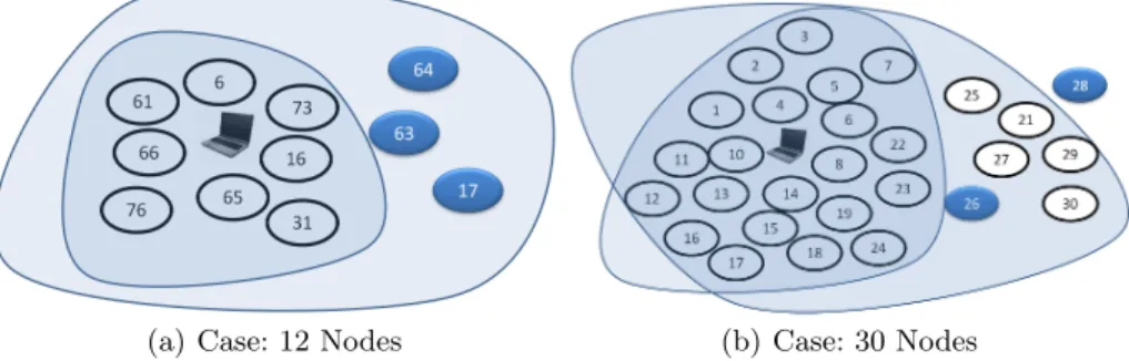
To validate the above hypothesis, we deployed rC-MHP in sparse (12 nodes) and dense (30 nodes) networks (5 m × 4 m). Fig. 6(a) Fig. 6(b) show the cluster-ing for rC-MHP. Some nodes durcluster-ing the initialization phase or after the BEA-CON TIME OUT phase declare themselves as CHs. If the node detects that it is under other CH and looses the contention, it sends a burst of special messages stating “I am no longer a CH”.
In case of sparse network (Fig. 6(a)), mostly, only a single CH (BS) could be observed. Sometimes, due to wireless channel problems or other factors such as BEACON TIME OUT, the nodes 17/63/64 declared themselves as CH(only one node at a time). The nodes in the Case 1 and 2 were deployed in similar conditions.
Similarly, in the case of a dense network (Fig. 6(b)), for most of the time, only a single cluster could be observed. Once during the experiments, due to
(a) Case: 12 Nodes (b) Case: 30 Nodes
Fig. 6: rC-MHP for different numbers of nodes in the same area
wireless channel problems or other factors such as BEACON TIME OUT, the node 28 declared itself as a CH and few other nodes joined it (only one node at a time). To summarize, the node density has no effect on rC-MHP, hence rC-MHP behaves like a scalable algorithm.
3.3 rC-MHP and Max-Min in large network
(a) rC-MHP (b) Max-Min
Fig. 7: Location of Cluster Heads
The Fig. 7(a) and Fig. 7(b) illustrate the positions of CHs when 63 sensors were deployed in an area of 17m × 27m. The transmission power was set to −20dbm and the threshold LQI was 106. In case of rC-MHP, we can see that the distribution of the CHs is regular while in case of Max-Min the CHs distribution is not ordered. It is due to the fact that, in case of rC-MHP, only one node can remain CH in its area of influence. Since the sensors are regularly distributed, the result is uniform, while in Max-Min it depends on the last phase.
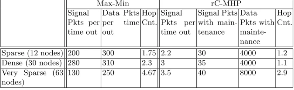
Table 2: Average number of clusters, data packets and hop counts per node. Max-Min rC-MHP Signal Pkts per time out Data Pkts per time out Hop Cnt. Signal Pkts per time out Signal Pkts with main-tenance Data Pkts with mainte-nance Hop Cnt. Sparse (12 nodes) 200 300 1.75 2.2 30 4000 1.2 Dense (30 nodes) 280 310 2.3 3 35 4000 1.1 Very Sparse (63 nodes) 130 250 4.67 3.5 40 8000 2.9
3.4 rC-MHP Vs Max-Min - Performance Analysis
We compare rC-MHP and Max-Min based on the overhead to create and main-tain clusters. Therefore, our performance criterion is “Number of Cluster/Phase messages” per data packets. The Table 2 compares the performance of rC-MHP with Max-Min. In Max-Min, increasing node density resulted in a higher num-ber of phases messages. For rC-MHP, the relative numnum-ber of phase messages remained the same.
The sensor nodes were switched ON at different time. So, they entered dif-ferent phases at difdif-ferent time. Therefore, Max-Min needed more time with high numbers of redundant phase messages to fully diffuse its clustering criteria. So, the number of phase messages increased along with number of neighbors. On average, after sending close to 300 data packets, at least one node in the net-work experienced a BEACON TIME OUT. So, the clustering procedure had to be repeated which increased the overhead. For the large network, nodes were spread over a larger area. Therefore the node density decreased, hence the rela-tive number of cluster messages decreased.
From Table2, it can be easily seen that rC-MHP easily outperforms Max-Min. rC-MHP is independent of the node density. For sparse networks, only 30 cluster messages were needed to send 4000 (approx.) data packets. Even in the larger networks, only 40 cluster messages were used to send close to 8000 data packets. In rC-MHP, the cluster head maintenance is in-built. Very few messages were needed by using the underlying CSMA to convey the message “I am no longer a CH” or “I am a CH”. Of course, there were several BEACON TIME OUT but we did not need to redo the clustering. So, it resulted into lesser cluster/signal packets. In case of Max-Min, the heuristic had to be rerun.
We mainly focused on the number of clusters in the network. As expected, the average hop count is also lower for rC-MHP than for Max-Min. So, rC-MHP consumes less energy. Though, we have not observed any problem for rC-MHP during the experiments with 65 sensors, we do intend to extend this work via simulations on large scale.
Complexity: Max-Min has a O(n × d) memory requirement where n is the number of neighbors while rC-MHP needs only 4 bytes for clustering. On a real implementation, Max-Min needed 4 Timers while rC-MHP needed one Timer.
4
Conclusion and Discussion
In this paper, we propose rC-MHP, a rapid clustering algorithm inspired from the Mat´ern Hardcore Process and implement it on Tmote Sky sensors. rC-MHP does not need to store any information of its immediate neighbors so it is very practical. It is very simple to code on sensors. It does not need much synchro-nization between the nodes, hence it can be concluded that rC-MHP is a natural algorithm which can be used with CSMA. We compare it with Max-Min clus-ter algorithm and empirically show that the clusclus-tering overhead for rC-MHP is negligible and it is feasible in real sensors. rC-MHP inherently does the cluster maintenance. For rC-MHP no memory is required for clustering (except for the clusterhead and the routing table) and the number of cluster messages does not increase with the node density.
References
1. Becker, M., Beylot, A.L., Dhaou, R., Gupta, A., Kacimi, R., Marot, M.: Exper-imental study: Link quality and deployment issues in wireless sensor networks. Networking 2009, Aachen, Germany (May 2009)
2. Gupta, A., Diallo, C., Marot, M., Becker, M.: Understanding topology challenges in the implementation of wireless sensor network for cold chain. IEEE Radio and wireless symposium, RWS2010, New Orleans, USA (January 2010)
3. Woo, A., Tong, T., Culler, D.: Taming the underlying challenges of reliable mul-tihop routing in sensor networks. SenSys (2003)
4. Stoyan, D., Kendall, W.S., Mecke, J.: Stochastic Geometry and Its Applications, 2nd Edition. (September 1995)
5. Amis, A., Prakash, R., Vuong, T., Huynh, D.: Max-min d-cluster formation in wireless ad hoc networks. In: Nineteenth Annual Joint Conference of the IEEE Computer and Communications Societies. (2000)
6. De Clauzade De Mazieux, A.D., Marot, M., Becker, M.: Correction, gener-alisation and validation of the ”max-min d-cluster formation heuristic”. In: NETWORKING-07: Proceedings of the 6th international IFIP-TC6 conference on Ad Hoc and sensor networks, wireless networks, next generation internet, Berlin, Heidelberg, Springer-Verlag (2007) 1149–1152
7. Baccelli, F., B laszczyszyn, B., M¨uhlethaler, P.: An aloha protocol for multihop mobile wireless networks. IEEE Transactions on Information Theory 52 (2006) 421–436
8. Hoydis, J. andPetrova, M., Mahonen, P.: Effects of topology on local throughput-capacity of ad hoc networks. In: Personal, Indoor and Mobile Radio Communica-tions, 2008. PIMRC 2008. IEEE 19th International Symposium on. (2008) 9. : Ieee std. 802.15.4 - 2003: Wireless medium access control (mac) and physical
layer (phy) specifications for low rate wireless personal area networks (lr-wpans) 10. Srinivasan, K., Levis, P.: Rssi is under appreciated. Third Workshop on Embedded
Networked Sensors, EmNets (2006)
11. Gupta, A., Sharma, M., Marot, M., Becker, M.: Hybridlqi: Hybrid multihoplqi for improving asymmetric links in wireless sensor networks. The Sixth Advanced International Conference on Telecommunications, Barcelona, Spain (9 - 15, May 2010)