Automatic Optimization of Sparse Tensor Algebra
Programs
by
Ziheng Wang
Submitted to the Department of Electrical Engineering and Computer
Science
in partial fulfillment of the requirements for the degree of
Master of Engineering in Electrical Engineering and Computer Science
at the
MASSACHUSETTS INSTITUTE OF TECHNOLOGY
May 2020
c
○ Massachusetts Institute of Technology 2020. All rights reserved.
Author . . . .
Department of Electrical Engineering and Computer Science
May 18, 2020
Certified by . . . .
Saman Amarasinghe
Professor of Electrical Engineering and Computer Science
Thesis Supervisor
Accepted by . . . .
Katrina LaCurts
Chair, Master of Engineering Thesis Committee
Automatic Optimization of Sparse Tensor Algebra Programs
by
Ziheng Wang
Submitted to the Department of Electrical Engineering and Computer Science on May 18, 2020, in partial fulfillment of the
requirements for the degree of
Master of Engineering in Electrical Engineering and Computer Science
Abstract
In this thesis, I attempt to give some guidance on how to automatically optimize programs using a domain-specific-language (DSLs) compiler that exposes a set of scheduling commands. These DSLs have proliferated as of late, including Halide, TACO, Tiramisu and TVM, to name a few. The scheduling commands allow suc-cinct expression of the programmer’s desire to perform certain loop transformations, such as strip-mining, tiling, collapsing and parallelization, which the compiler pro-ceeds to carry out. I explore if we can automatically generate schedules with good performance.
The main difficulty in searching for good schedules is the astronomical number of valid schedules for a particular program. I describe a system which generates a list of candidate schedules through a set of modular stages. Different optimization decisions are made at each stage, to trim down the number of schedules considered. I argue that certain sequences of scheduling commands are equivalent in their effect in partitioning the iteration space, and introduce heuristics that limit the number of permutations of variables. I implement these ideas for the open-source TACO system. I demonstrate several orders of magnitude reduction in the effective schedule search space. I also show that for most of the problems considered, we can generate schedules better than or equal to hand-tuned schedules in terms of performance.
Thesis Supervisor: Saman Amarasinghe
Acknowledgments
I would like to thank Saman Amarasinghe and Fredrik Kjolstad for all the support and mentorship in the past year. I would also like to thank Ryan Senanayake, Stephen Chou and Changwan Hong for their helpful discussion and insights. Finally I would like to acknowledge the support from all of my family and friends.
Contents
1 Introduction 15
2 Scheduling Framework 23
2.1 Background . . . 23
2.2 The Hypercube Perspective . . . 24
2.3 Dense Partition . . . 26
2.3.1 Addressing Fuse . . . 29
2.4 Sparse Partition . . . 34
2.5 Reordering and Parallelism . . . 40
2.5.1 Trimming Passes . . . 43 2.5.2 CPU . . . 45 2.5.3 GPU . . . 47 2.6 Search . . . 51 3 Evaluation 53 3.1 SpMV . . . 55 3.2 SpMM . . . 59 3.3 MTTKRP . . . 62
3.4 Analysis and Future Work . . . 64
4 Discussion and Related Work 69
List of Figures
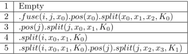
1-1 a) The autoscheduler has a sequence of stages, where each stage emit possible choices for the next stage to explore further. b) If we restrict some choices at some intermediate stage, it can greatly affect the num-ber of schedules generated in the end. Generally the earlier we restrict choices the greater effect we have. . . 17 1-2 A visual illustration of the space of schedules. Each schedule template
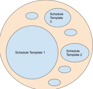
can generate a family of schedules, by changing the values of the tun-able parameters. Different schedule templates can generate families of different sizes. Therefore, eliminating one schedule template might have a substantially larger effect on reducing the search space than eliminating another. . . 18
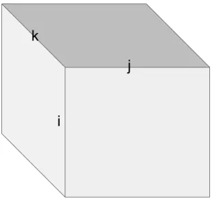
2-1 The hypercube corresponding to matrix multiplication 𝐶(𝑖, 𝑘) = 𝐴(𝑖, 𝑗)× 𝐵(𝑗, 𝑘). If we discretize the edges, then this hypercube defines a grid of points, which correspond to the multiplication operations. This is exactly the same as in the Polyhedral model. Some points might not have to be visited if they correspond to multiplication by zero in the sparse case. . . 25 2-2 How we can induce a partition in 2 dimensions by partitioning each
1 dimensional-edge: 𝜋(𝑥1, 𝑥2) = (𝜋(𝑥1), 𝜋(𝑥2)).Higher dimensions are
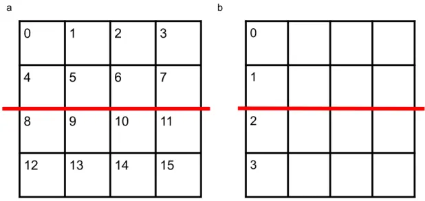
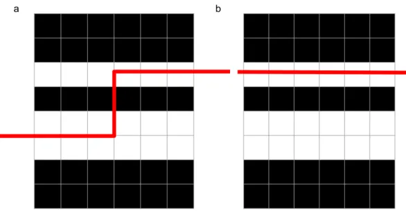
2-3 a) Splitting after fusing 𝑋0 and 𝑋1. b) Splitting just one axis and
projecting this partition across the other one. We see that splitting the fused coordinate space of size 16 is equivalent to splitting just along one axis of size 4, and projecting that split across the other axis. 31 2-4 A comparison of two strategies. a) less choices at earlier stages could
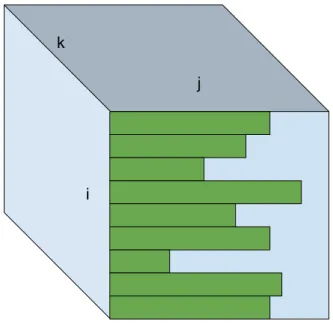
lead to potential redundant schedules in the end while b) more choices at earlier stages could actually lead to fewer viable schedules in the end. 34 2-5 What the hypercube looks like is one of the dimensions, 𝑗 is sparse,
with corresponding dimension 𝑖. . . 35 2-6 This is what a compressed-dense iteration space looks like. a) the result
from splitting after fuse. b) the result if just splitting the compressed dimension. As we can see, it’s quite similar, up to some difference bounded by the size of the dense dimension. If the compressed dimen-sion has an even number of nonzeros, then it would’ve been exactly the same. . . 39 3-1 The results from trimming the search space of SpMV schedules for a)
CPU and b) GPU. . . 56 3-2 Runtimes for cuSPARSE, Merge SpMV, handtuned scheduled TACO
and autoscheduled TACO . . . 57 3-3 Runtimes for cuSPARSE, Merge SpMV, handtuned scheduled TACO
and autoscheduled TACO . . . 58 3-4 The results from trimming the search space of SpMM schedules for a)
CPU and b) GPU. . . 59 3-5 SpMM runtimes for cuSPARSE, handtuned scheduled TACO, and
au-toscheduled TACO. . . 60 3-6 SpMM runtimes for cuSPARSE, handtuned scheduled TACO, and
au-toscheduled TACO. . . 61 3-7 The results from trimming the search space of MTTKRP schedules for
3-8 B-CSF Kernel by Nisa et al., handtuned schedule and autoscheduled TACO performance on 4 tensors. . . 64 3-9 Bubble chart with more details filled in. The green circles represent
the different schedules generated from the same schedule template. Note that schedule templates from different split schedules can generate different numbers of schedules because they have a different number of tunable parameters. . . 65 3-10 Distributions of runtimes for SpMM for cage15 matrix on CPU.
Differ-ent colors correspond to differDiffer-ent split schedules. Some colors overlay almost exactly on each other. . . 66 3-11 Distributions of runtimes for SpMM for Si41Ge41H72 matrix on CPU.
List of Tables
2.1 Applicability 𝑓 𝑢𝑠𝑒 on 𝑋1 and 𝑋2 depending on their formats and if
they belong to the same tensor. . . 40 3.1 SpMV split schedules . . . 56 3.2 SpMM split schedules . . . 59
Chapter 1
Introduction
In recent years, many domain specific languages (DSLs) have been developed to de-scribe scientific or machine learning computations. These DSLs typically target pro-grams that can be expressed as loop nests. For example, the pairwise forces compu-tation in molecular dynamics simulations involve a double for loop over all the atoms. Image filtering algorithms involve 2D stencil computations which can be expressed as a double for loop over the filter elements. Notable recent DSLs include Halide (originally developed for image processing), TACO (sparse tensor algebra), Tiramisu (sparse/dense linear algebra) and TVM (deep learning) [18, 3, 5, 10].
In addition to a language to describe the computation using an algorithmic lan-guage, these recent DSLs typically include a way to describe the concrete implementa-tion of the algorithm, which is called a schedule. A specificaimplementa-tion of the computaimplementa-tion and the schedule completes the program. The idea is that programmer can change the schedule without impacting the computation, which allows rapid experimentation with different implementations to find the fastest one [17]. The ease of performance engineering is arguably why these DSLs exist. A lot of recent effort has focused on autoscheduling—automatically finding the best schedule for the DSL for a specific computation to get the best performance. The autoscheduler searches through the space of possible schedules to find the best. [13, 1]
A schedule is typically expressed by a sequence of scheduling commands, exposed by the scheduling API of the DSL, for example, unroll, reorder, or parallelize [18,
10]. These scheduling commands effect different loop transformations in the DSL. Many recent DSLs adopt this approach, including Halide, TACO, Tiramisu and TVM. Different systems go to different depths on autoscheduling. TVM for example, needs the user to manually specify the AST (template in TVM parlance). Auto-TVM then proceeds to find the best parameters for this template, i.e. tile size, block size etc [6]. The latest Halide autoscheduler generates this tree using a machine learning approach, trained on billions of fake programs [1].
The autoscheduler could be viewed as a compiler. Whereas a traditional compiler translates a piece of code into a sequence of instructions, the autoscheduler translates a tensor algebra problem into a sequence of these scheduling commands.
Modern compilers are designed with multiple optimization passes. These opti-mization passes makes the compiler modular and extensible. Each optiopti-mization pass produces an intermediate representation of the original piece of code. These interme-diate representations contain strictly more detail than the original code – they encode choices made by the compiler at each stage to optimize the performance.
In this thesis, I will present autoscheduler whose design is inspired by the multi-stage heuristics-based optimizations in modern compilers, in contrast with the one-shot machine learning approaches typically employed today. Starting from a problem described in the tensor algebra notation, it makes a sequence of decisions, which in-crementally specify more and more of the schedule. The sequence of decision involves how to partition the iteration space, how to reorder the index variables, which vari-ables to parallelize, and finally what values tunable parameters take. At each step in this sequence, there are multiple choices to explore, expanding upon which we get even more choices at the next step, as shown in Figure 1-1a.
The first major stage is the generation of a list of schedule templates. A schedule template is a schedule without parameters such as split factors filled in, a.k.a. a loop transformation strategy without parameters. This stage could be divided into two substages: partition and assignment. In the first substage I decide how to cut up the iteration space. The second substage decides how to iterate over and through the chunks. We will go through this in detail later.
Figure 1-1: a) The autoscheduler has a sequence of stages, where each stage emit possible choices for the next stage to explore further. b) If we restrict some choices at some intermediate stage, it can greatly affect the number of schedules generated in the end. Generally the earlier we restrict choices the greater effect we have.
The second stage is filling in the numbers in each schedule template to generate schedules that can be lowered into code using a DSL. Needless to say, each schedule template can correspond to multiple schedules.
These two stages generate a list of candidate schedules. One now has to search through all the schedules we have generated. There are many approaches in literature, from recent neural network based approaches such as [6] to decades-old approaches like Thompson sampling. Figure 1-2 provides a visual description of the search space. There is some confusion in the field pertaining to exactly what autoscheduling entails. Some works, for example autoTVM, define autoscheduling to be finding the best parameters for a fixed schedule template [5]. More recent works, [1] define autoscheduling to also include the generation of the schedule template. Similarly, in this work, I aim to both generate the schedule template and the schedule.
The key challenge in autoscheduling is that the list of viable schedules for a par-ticular problem is often astronomically large. As a thought example, let’s imagine
Figure 1-2: A visual illustration of the space of schedules. Each schedule template can generate a family of schedules, by changing the values of the tunable parameters. Different schedule templates can generate families of different sizes. Therefore, elimi-nating one schedule template might have a substantially larger effect on reducing the search space than eliminating another.
generating schedules for a particular program, say sparse matrix dense vector multi-plication: 𝑦(𝑖) = 𝐴(𝑖, 𝑗) × 𝑥(𝑗). This is probably one of the simplest sparse tensor algebra problems. In TACO, there are at least 1000 legal schedule templates for this simple program. each of these schedule templates contains one or more parameters. Assuming that there are at least three choices for each parameter, then each schedule template can give rise to at least three schedules. The search algorithm at the end would have to explore a space of three thousand schedules. If we assume that exe-cuting a single schedule takes three seconds, then searching through this entire space would take more than 2 hours. More complicated sparse tensor algebra problems can take significantly longer. One could invest a lot of effort into a good search algorithm that navigates this space efficiently, such as autoTVM or OpenTuner [5, 2]. To com-plement those approaches, we can also invest some effort into reducing the search space size.
The key to reducing the search space size is restricting the set of optimizations explored at each stage and substage, so that the total number of possible schedules generated at the end is small enough for the search to be feasible, as illustrated in Fig-ure 1-1b. We will design these stages based on an understanding of the computation we are scheduling and the hardware we are targeting. I design the stages to be largely independent of each other. For the total number at the end to be small, the number of choices at each stage should be limited as much as possible. This means we can either generate fewer schedule templates, or we can limit the number of parameter choices for each schedule template. I claim that the first option is a lot more viable than the second option. It is difficult to claim that a set of legal parameter choices is better than another set of legal parameter choices for a particular schedule, assuming no knowledge of the input data and underlying hardware. However, it is relatively easier to claim that a particular schedule template is better than another schedule template, even without the parameter values filled in.
I now justify the counter-intuitive assertion I made at the end of the last para-graph. The schedule template makes qualitative statements about the properties of a schedule, while the actual parameters determine quantitative aspects. For example, the schedule template typically determines if a schedule is load-balanced, whereas the actual parameters might determine the amount of parallelism the schedule ex-poses. The schedule template determines the overall tiling strategy and iteration order, whereas the actual parameters determine the tile sizes. It is much harder to reason about the attractiveness of quantitative properties of schedules, whereas it’s much easier to reason about their qualitative aspects. While quantitative properties can be used to drive the machine learning systems to search the schedule space, simple heuristics can be derived from qualitative properties to drastically reduce the search space size.
Let’s now list some characteristics of bad schedule templates that we wish to eliminate. The first type is illegal schedule templates that simply do not compile in the DSL. On the grand scheme of things, they are actually not that bad, since if they never compile, we will not have to search parameters for them. However, they can
clutter up the schedule space, making meaningful analysis difficult. The second type is redundant schedule templates. This means two, or a group of, schedule templates all generate the same code. This scenario is painfully common in a lot of scheduling languages. Naive autoschedulers for example, could get caught endlessly reordering a couple of variables back and forth. How bad it is depends on how big the redundant group size is, and how large the parameter search space for each of those schedule templates is. The third type is inefficient schedule templates, which are almost certainly slower than some other schedule template. How bad they are correlate directly with how big their parameter search spaces are. A fundamentally flawed schedule template that captures a significant proportion of the final schedule search space is like a black hole that even the best search algorithms might have difficulty escaping from. For example, in Figure 1-2, half of the schedule space is derived from schedule template 1. If schedule template 1 is bad, then it would present such a “black hole”.
Illegal schedule templates can be removed by following the scheduling language’s rules. Redundant schedule templates can be removed by establishing functional equivalences between different sequences of schedule commands. These two types of schedule templates are relatively easy to remove. It is much harder, comparatively, to remove inefficient schedule templates. To do so, we have to introduce subjective criteria that good schedules probably fulfill, a.k.a. heuristics.
Up to this point, I have been talking in the context of some generic scheduling language and some generic DSL. While I hope the ideas I describe below can apply to many if not all of them, I will focus in particular on the DSL TACO [10]. TACO caters to sparse tensor algebra programs, which can be described by index notations [10]. I refer the unfamiliar reader to the multiple TACO publications for more information [10, 9, 7]. The scheduling API is described in [20].
In the following chapters, I will first describe the different stages of the autosched-uler in sequence (Chapter 2). I will first deal with partitioning dense and sparse itera-tion spaces into chunks in Secitera-tions 2-4. We will see that seemingly different sequences of scheduling commands can all describe virtually identical partition strategies. After
partitioning, we are left with a list of derived index variables from the original index variables. We will then explore how to reorder these derived index variables and parallelize them. We will find that the number of unique choices here are overwhelm-ing even for the simplest of problems. To address this, I design hardware-specific trimming passes to eliminate inefficient reordering and parallelization strategies in Section 5. Finally, we will describe how one can search through all the schedules gen-erated, treating the problem in an hierarchical multi-arm bandit setting in Section 6. In Chapter 3, I will evaluate my approach on three different sparse tensor algebra problems, SpMV, SpMM and MTTKRP on CPU and GPU. I will summarize my approach and compare it to related works in Chapter 4.
My specific contributions in this thesis are:
1. described heuristics to limit the number of strategies to partition sparse and dense iteration spaces into chunks
2. described heuristics to limit the number of ways to iterate through and paral-lelize the chunks
3. constructed an automated system that implements these heuristics to automat-ically write schedules for sparse tensor algebra problems in TACO.
Chapter 2
Scheduling Framework
2.1
Background
Before we start, let’s discuss the TACO scheduling API we have at our disposal. For more detail, the reader is referred to [19, 20]. As mentioned before, TACO is primar-ily intended for sparse tensor algebra, and has scheduling commands to transform dense and sparse loops. A sparse tensor algebra problem can be expressed in index notation, e.g. 𝑥(𝑖) = 𝐴(𝑖, 𝑗) × 𝑦(𝑗) for sparse matrix dense vector multiplication, where 𝐴 is a matrix in the CSR format. 𝑖 and 𝑗 are called index variables. The ranges of the index variables define the iteration space of the program. They can either be dense, like 𝑖, or compressed, like 𝑗. We will discuss the subtleties involved in scheduling compressed loops in more detail later on. The important commands that we need to know are:
1. 𝑟𝑒𝑜𝑑𝑒𝑟: swaps the order of iteration over two or more directly nested index variables (permutes the order of for loops).
2. 𝑠𝑝𝑙𝑖𝑡: splits (strip-mines) an index variable into two nested index variables, where the size of the inner index variable is constant. We call the two nested index variables derived index variables.
3. 𝑑𝑖𝑣𝑖𝑑𝑒: same as split, except that it’s the size of the outer index variable that is constant instead of the inner one.
4. 𝑓 𝑢𝑠𝑒: collapses two directly nested index variables, resulting in a new fused index variable that iterates over the product of the coordinates of the fused index variables.
5. 𝑝𝑎𝑟𝑎𝑙𝑙𝑒𝑙𝑖𝑧𝑒: parallelizes a loop over a parallel unit, e.g. OpenMP thread, GPU block or GPU thread.
Compressed loops can be scheduled in the coordinate space or the position space, via the 𝑝𝑜𝑠 scheduling command. We will talk about position space later.
Now that we have introduced the terminology and listed the scheduling commands, this chapter will proceed to examine how we can use them to partition dense and sparse iteration spaces. We will largely explore the partitioning from a geometrical perspective, which will assist us in weeding out redundant schedules which express the same partitioning strategy with different sequences of scheduling commands.
2.2
The Hypercube Perspective
Let’s take the example of matrix multiplication. The index notation is 𝐶(𝑖, 𝑘) = 𝐴(𝑖, 𝑗) × 𝐵(𝑗, 𝑘). We can represent the iteration space with a cube, as illustrated in Figure 2-1. (Instead of a cube which suggest a solid object, perhaps I should empha-size that it’s a 3D grid of points. In the following discussion, "cube" is implicitly understood to be this 3D grid of points.) Each edge corresponds to an index variable in the problem. The first matrix, which is sparse, is represented by the face with the edges i and j, where j is the sparse dimension. The second matrix, which is dense, is represented by the face with edges j and k. Each point inside this cube represents an individual multiplication. Since the problem is sparse, we do not need to iterate over every point inside the cube. Problems with more than 3 index variables can natually be represented by higher order hypercubes. This is a very polyhedral view of the world. A lot of disciples of this doctrine have written much better and possibly more lucid explanations of this perspective [27, 4]. This polyhedral per-spective allows to visualize what partition strategies described by different sequences
Figure 2-1: The hypercube corresponding to matrix multiplication 𝐶(𝑖, 𝑘) = 𝐴(𝑖, 𝑗) × 𝐵(𝑗, 𝑘). If we discretize the edges, then this hypercube defines a grid of points, which correspond to the multiplication operations. This is exactly the same as in the Polyhedral model. Some points might not have to be visited if they correspond to multiplication by zero in the sparse case.
of scheduling commands do to iteration space, which will help us in weeding out redundant schedules.
We are faced with the task of taking this cube, which describes the sparse tensor algebra problem, and specifying how it is to be actually carried out on our hardware, be it CPU or GPU or potentially some FPGA accelerator. What does this entail? Assuming we have some parallel hardware device, then we have to specify for each point in this cube, two important attributes: which processor the point executes on and when it is to be executed on said processor among all the points assigned to it. The problem of autoscheduling can be thought of specifying these two things, for all the points in the hypercube.
It’s important to note that the polyhedral model cares greatly about dependencies between execution instances, i.e. points inside the cube. If some points must occur after other points for example, then the number of transformations one can make
to the cube are greatly restricted. Fortunately, in tensor algebra problems, all of the execution instances are independent of one another. All of the multiplications in the problem can occur in any order or all at once, before the reductions happen. The reductions can also be done in any order. We thus do not have to worry about dependency analyses here, though it can potentially be introduced into my approach if necessary.
2.3
Dense Partition
In this section, we show how to think about partitioning a dense iteration space with the commands 𝑓 𝑢𝑠𝑒, 𝑠𝑝𝑙𝑖𝑡 and 𝑑𝑖𝑣𝑖𝑑𝑒. We show that the command 𝑓 𝑢𝑠𝑒 is effectively redundant, and we can proceed to partition each index variable independently using 𝑠𝑝𝑙𝑖𝑡 and 𝑑𝑖𝑣𝑖𝑑𝑒.
Before we proceed further, let’s attempt to establish a formalism that describes the splitting we are going to be doing. Let us assume that the problem we are interested in have 𝑛 index variables, which are called 𝑋1, 𝑋2, ..., 𝑋𝑛. Let’s use |𝑋𝑖|
to denote the maximum value that index variable can take (iteration bound). For a moment, let’s assume that we cannot fuse dimensions. Then our job is to specify partitions 𝜋1.𝜋2...𝜋𝑛to divide up the index variables. A partition is a function defined
as 𝜋𝑖 : {0, 1...|𝑋𝑖|} → {0, 1...𝑑𝑖}, where we divide the range of index variable 𝑋𝑖 into
𝑑𝑖 non-overlapping subsets. Henceforth, we will abbreviate {0, 1...𝑥} as 𝑟𝑎𝑛𝑔𝑒(𝑥).
Because the domain of 𝜋𝑖 is discrete, we can also describe it as a sequence composed
of its action on each element in 𝑟𝑎𝑛𝑔𝑒(|𝑋𝑖|): (𝜋𝑖(0), 𝜋𝑖(1)..., 𝜋𝑖(|𝑋𝑖|)).
The partitions on each edge induce a straightforward partition of the hypercube 𝜋 : ∏︀𝑛
𝑖=1𝑟𝑎𝑛𝑔𝑒(𝑋𝑖) → ∏︀𝑛𝑖=1𝑟𝑎𝑛𝑔𝑒(𝑑𝑖) through projection, as shown in Figure 2-2.
This partitions the hypercube into ∏︀𝑛
𝑖=1𝑑𝑖 partitions. We can assign an 𝑛 long tuple
to each point in the cube specifying which partition it is in.
Let us focus on one single index variable, 𝑋𝑖 and think about what does 𝜋𝑖 have
to be. In particular, we’d like to gain some intuition regarding what 𝜋𝑖 should look
Figure 2-2: How we can induce a partition in 2 dimensions by partitioning each 1 dimensional-edge: 𝜋(𝑥1, 𝑥2) = (𝜋(𝑥1), 𝜋(𝑥2)).Higher dimensions are analogous.
massive. We’d like to restrict our attention to partitions that are 1) meaningful and likely to be useful and 2) achievable using a scheduling language.
Let’s first consider the second condition, because it’s much easier to reason about. What tools do we have to construct such a partition? As alluded to before we cannot just arbitrarily specify this function. Let’s consider a scheduling function with two commands: split and divide. Split is a command that divides a loop into fixed sized inner loops, whereas divide divides a loop into a fixed number of outer loops. For more information, please refer to [20]. For example, 𝑠𝑝𝑙𝑖𝑡(𝑋𝑖, 𝑥0, 𝑥1, 4) will produce
the following code (assuming that |𝑋𝑖| is divisible by 4):
f o r x0 = 0 . . . | Xi | / 4 f o r x1 = 0 . . . 4
Whereas 𝑑𝑖𝑣𝑖𝑑𝑒(𝑋𝑖, 𝑥0, 𝑥1, 4) will produce the following code:
f o r x0 = 0 . . . 4
It is straightforward to see that the first command will produce the following partition on 𝑟𝑎𝑛𝑔𝑒(𝑋𝑖) :
(1, 1, 1, 1, 2, 2, 2, 2, 3, 3, 3, 3...|𝑋𝑖|/4, |𝑋𝑖|/4, |𝑋𝑖|/4, |𝑋𝑖|/4)
It’s important to see that the first command can also be used to produce another partition:
(1, 2, 3, 4, 1, 2, 3, 4...1, 2, 3, 4).
Let’s call 𝑥0 and 𝑥1 derived index variables. The first partition implicitly
as-sumes that we index the partitions with 𝑥0. However, we could also index the
chunks with 𝑥1. If we insist that in a two-level loop, the outer loop iterates over
the chunks and the inner loop iterates within a chunk, then this could be described by 𝑠𝑝𝑙𝑖𝑡(𝑋𝑖, 𝑥0, 𝑥1, 4).𝑟𝑒𝑜𝑟𝑑𝑒𝑟(𝑥1, 𝑥0). This reorder can always be done, since the
iteration bounds of the two variables being reordered are completely independent. This partition illustrates that the partition doesn’t necessarily have to be contigu-ous. What does the 𝑑𝑖𝑣𝑖𝑑𝑒 command produce?
(1, 1, 1...1, 2, 2, 2...2, 3, 3, 3...3, 4, 4, 4...4) and
(1, 2, ...|𝑋𝑖|/4, 1, 2, ...|𝑋𝑖|/4, 1, 2, ...|𝑋𝑖|/4, 1, 2, ...|𝑋𝑖|/4, ).
In short, the 𝑠𝑝𝑙𝑖𝑡 command can produce a data dependent number of fixed size contiguous chunks indexed by 𝑥0and a fixed number of data dependent sized
noncontiguous chunks indexed by 𝑥1. Noncontigous means that the elements in the
chunk are not adjacent in memory, which could result in unfavorable spatial locality properties. The 𝑑𝑖𝑣𝑖𝑑𝑒 command can produce a data dependent number of fixed size noncontiguous chunks indexed by 𝑥1 and a fixed number of data dependent sized
contiguous chunks indexed by 𝑥0. I advise the reader to spend a moment reflecting
upon this.
To summarize, a partition can be characterized by three things: 1) whether or not the number of disjoint sets, 𝑑𝑖, is statically known. 2) whether or not the size of each
disjoint set is statically known. 3) whether or not the disjoint sets are contiguous. All three describe important qualitative aspects of the schedule, and will play an important role in heuristics used to eliminate inefficient schedules. Let’s give a preview here. In some parallel models, there are a limited number of parallel units available.
If we are to assign each disjoint set in the partition to a parallel unit, then we need to know the number of disjoint sets statically to ensure that there is sufficient parallel resources. Sometimes, parallel units strongly prefer to operate over a contiguous set of points in the hypercube, e.g. due to memory locality. Then we would prefer the disjoint sets to be contiguous.
Of course, all this discussion about data dependent loop bounds assumes that we do not know what |𝑋𝑖| is at compile time. If we do know, then it’s evident that these
two commands or more or less equivalent to each other. Both can produce either a fixed number of fixed size noncontiguous chunks or a fixed number of fixed size contiguous chunks. Some scheduling languages allow for user input of this kind of information. For example, we could use the 𝑏𝑜𝑢𝑛𝑑 command in TACO to explicitly specify what the value of a data dependent number is.
Obviously, there are other forms 𝜋𝑖could take, for example (1, 1, 2, 2, 3, 3, 1, 1, 2, 2, 3, 3...).
This partition strategy is achievable through repeatedly applying the 𝑠𝑝𝑙𝑖𝑡 command. In fact, we can apply these four partition strategies above recursively and without end in an infinite loop to effect the death of any autoscheduler.
To simplify our discussion, let’s restrict our attention to only these four partition strategies for now. We also include a fifth strategy, which just leaves the index variable as is. While this could be expressed as 𝑠𝑝𝑙𝑖𝑡(𝑋𝑖, 𝑥0, 𝑥1, 1), writing
it this way produces overhead in the resulting code and could lead to overcounting the number of schedules in the end. This point will be elaborated on further later on. It is straightforward now to imagine that if each dimension of this hypercube is split in one of these five strategies, we could project the partitions to form a partition of the hypercube itself.
2.3.1
Addressing Fuse
Now let’s think about the 𝑓 𝑢𝑠𝑒 command. What does this do? Let’s imagine that we can fuse some subsets of the index variables 𝑋1, 𝑋2, ..., 𝑋𝑛. Does that increase the
repertoire of partitions of the hypercube at our disposal?
new axis 𝐹 . Now we can apply our four partition types to this axis 𝐹 . We realize that none of the strategies actually produce a partition that is substantially different from what we can obtain from just partitioning the two axes independently. How so? Let’s imagine the two partitions produced by 𝑠𝑝𝑙𝑖𝑡. Consider 𝑠𝑝𝑙𝑖𝑡(𝐹, 𝑥0, 𝑥1, 𝐾). To
simplify our analysis, let’s assume that |𝑋1| and |𝑋2| and 𝐾 are all powers of two.
Let’s just consider the case where the chunks are contiguous.
Then there are two cases. The first case is if 𝐾 ≤ |𝑋2|. In this case, we
re-alize that the resulting partition pattern can be achieved without fuse, by splitting the two axes separately and considering their projection, i.e. 𝑠𝑝𝑙𝑖𝑡(𝑋1, 𝑥11, 𝑥12, 1).
𝑠𝑝𝑙𝑖𝑡(𝑋2, 𝑥21, 𝑥22, 𝐾). Note that the projection would create a 2-D array of chunks
indexed by 𝑥0 and 𝑥2, whereas splitting 𝐹 would have resulted in a 1-D array of
chunks, indexed by 𝑥0. This is just a technical difficulty that could be resolved
post-facto by fusing 𝑥0 and 𝑥2 in the former case. The second case is if 𝐾|𝑋2|. In this
case, the equivalent operation is simply 𝑠𝑝𝑙𝑖𝑡(𝑋1, 𝑥11, 𝑥12, 𝐾/|𝑋2|). An example
il-lustration is shown in Figure 2-3. The argument for the case where the chunks are noncontiguous is exactly analogous. Note we could argue that we do not know the value of |𝑋2| at compile time, thus there is no way to produce the equivalent command
statically. However, as mentioned in Chapter One, the autoscheduler is preoccupied with producing a list of correct schedule templates, without the exact parameters filled in. We can assume that later, we will perform exhaustive autotuning on these parameters. As a result, though we cannot determine the value of 𝐾/|𝑋2| statically,
we can assume it will be explored in the autotuning process.
Now let’s consider 𝑑𝑖𝑣𝑖𝑑𝑒(𝐹, 𝑥0, 𝑥1, 𝐾). Again let’s consider the contiguous chunk
case. Again there are two cases. The first case is if 𝐾 ≤ |𝑋1|. Then in this case
we realize that the command is exactly equivalent to 𝑑𝑖𝑣𝑖𝑑𝑒(𝑋1, 𝑥0, 𝑥1, 𝐾). The
sec-ond case is if 𝐾 > 𝑋1. Then the command is equivalent to the following sequence
of commands 𝑠𝑝𝑙𝑖𝑡(𝑋1, 𝑥11, 𝑥12, 1).𝑑𝑖𝑣𝑖𝑑𝑒(𝑋2, 𝑥21, 𝑥22, 𝐾/|𝑋1|), followed by fusing 𝑥11
and 𝑥21. Similarly, the argument for the noncontiguous case is analogous.
For the fifth partition strategy where we don’t do anything to the fused variable, the fuse is then not particularly useful. In fact, it is probably harmful, because you
Figure 2-3: a) Splitting after fusing 𝑋0 and 𝑋1. b) Splitting just one axis and
pro-jecting this partition across the other one. We see that splitting the fused coordinate space of size 16 is equivalent to splitting just along one axis of size 4, and projecting that split across the other axis.
have to use the remainder and integer division operations to recover the original indices, which tend to be expensive on modern architectures.
We have just proved a rather significant result: in the dense case where things are powers of two, it is futile to consider fusion of 2 dimensions for expanding the number of ways to partition the 2-D iteration space. At most, we should only fuse the variables that are being used to index the chunks. In general, if things are not powers of two, this result will not hold exactly. However, one could show with some more complicated arithmetic that the sizes of the chunks in partitions of the fused variable are within a reasonable neighborhood of the sizes of the chunks achievable by partitioning both index variables independently. Let’s ignore this for the sa, and write down the following theorem. The precise formal language is not as important as the intuition in the proof I just described.
Theorem 1 Assuming |𝑋1|, |𝑋2| are powers of 2. The set of partitions that can be
with 𝐾 a power of 2 is contained in the set of partitions that can be achieved by partitioning 𝑋1 and 𝑋2 independently using one of the five strategies with 𝐾 a power
of 2, and projecting the result.
Following this theorem, we can use induction to prove the corollary, which asserts that 𝑓 𝑢𝑠𝑒 does not need to be considered for all 𝑛 dimensions.
Corollary 1.1 Assuming |𝑋1|, |𝑋2|...|𝑋𝑛| are powers of 2. The set of partitions that
can be achieved by fusing 𝑋1, 𝑋2...𝑋𝑛 and applying one of the five aforementioned
strategies is contained in the set of partitions that can be achieved by partitioning 𝑋1, 𝑋2...𝑋𝑛 independently using one of the five strategies, and projecting the result.
To prove this, we will use induction. The base case has been proven in Theorem 1. Let’s assume this corollary holds for 𝑋1, 𝑋2, ...𝑋𝑛−1. We see that 𝑓 𝑢𝑠𝑒(𝑋1, 𝑋2, ...𝑋𝑛)
can be broken down to be the fusion of two index variables 𝑓 𝑢𝑠𝑒(𝑋1, ...𝑋𝑛−1) and 𝑋𝑛.
By Theorem 1 all partitions on 𝑓 𝑢𝑠𝑒(𝑋1, 𝑋2, ...𝑋𝑛) can be expressed by projections of
partitions on 𝑓 𝑢𝑠𝑒(𝑋1, ...𝑋𝑛−1) and 𝑋𝑛. But by the induction hypothesis, partitions
of 𝑓 𝑢𝑠𝑒(𝑋1, ...𝑋𝑛−1) can be expressed as projections of partitions on 𝑋1, 𝑋2, ...𝑋𝑛−1.
Thus, all partitions on 𝑓 𝑢𝑠𝑒(𝑋1, 𝑋2, ...𝑋𝑛) can be expressed as projections of
parti-tions on 𝑋1, 𝑋2, ...𝑋𝑛.
Corollary 1.1 provides immense value to thinking about autoscheduling. We realize that partitioning the hypercube of a dense iteration space can be done one axis at a time without any interactions between them. This also suggests we can partition it in any order we see fit, since there is no dependence in the partitions specified for each independent index variable. Note that the corollary only establishes that the all partitions resulting from fusion can be produced from partitioning the index variables separately. It does not assert the opposite. In fact the opposite is not true: simply fusing all the index variables and partitioning that fused result will result in a loss of expressive power.
What does this suggest about the scheduling commands that we should issue? We see that for each index variable, we can use 𝑠𝑝𝑙𝑖𝑡 or 𝑑𝑖𝑣𝑖𝑑𝑒, and optionally reorder the resulting two variables. The analysis thus far has suggested that for 𝑋1, 𝑋2, 𝑋3, ..., 𝑋𝑛,
we should first partition each of them independently, producing up to 2𝑛 variables, up to 2 from each one of the original index variable. Whereas reordering the 2 variables resulting from partitioning one particular axis results in different partition strategies, we can actually reorder all 2𝑛 variables thus produced. In the dense case, there are no external restrictions on the order of iterations of the variables, since their iteration ranges do not depend on one another.
We might wish not to split a variable and easily repeat the following analysis with fewer than 2𝑛 variables. Then we will have to consider potentially up to 2𝑛 cases, where each variable could be split or not. This sounds unmanageable, but in reality 𝑛 is typically very small, so this is okay. The astute reader will note that we can encapsulate “not splitting” an index variable by splitting it with split factor 1. This suggests that if we allow the search process to explore split factor 1, then we can just split all the index variables in a single case, and then let the search process decide if some index variables shouldn’t be split after all. It seems like we should just produce a single schedule template with a bunch of split factors to fill in, and let the search process do its job, vs. produce a bunch of schedule templates with potentially fewer split factors to fill in, and search each of them.
While the latter strategy appears more complicated, it actually reduces the final search space. This is because if we allow a split factor of 1, then we are effectively introducing a useless loop into the schedule. However, we had already considered the set of valid permutations containing this loop, not knowing that it is useless. As a result, we will explore different permutations where the only difference is where this useless loop is executed in regards to other loops, and there is no difference. In short, some schedule templates might be redundant under certain parameter choices. This tradeoff is depicted visually in Figure 2-4.
The next question to be answered is how to globally reorder the up to 2𝑛 variables generated, and which of them to parallelize over. We will discuss that momentarily. Let’s first extend the above analysis to sparse iteration spaces.
Figure 2-4: A comparison of two strategies. a) less choices at earlier stages could lead to potential redundant schedules in the end while b) more choices at earlier stages could actually lead to fewer viable schedules in the end.
2.4
Sparse Partition
In the world of sparse linear algebra, where holes might exist in the cube, partitioning the cube such that each partition has the same number of points is an unattainable luxury. Cutting the cube like we did above for the dense case is now called scheduling in coordinate space. We can divide each edge of the cube evenly, and hope that the the holes are evenly distributed in this cube. Then, each slice of the cube will roughly have the same number of holes, or the same number of points for us to process. However, this usually doesn’t happen in sparse tensor algebra problems in science and engineering because the sparsity pattern is often highly structured.
We can get a bit creative, and perform cuts in the position space of an edge. What is a position space? It is described in detail in [20]. Briefly, you are partitioning the nonzeros of a dimension, guaranteeing that each partition has the same number of nonzeros. This kind of cutting has a lot of subtleties, an important one of which is that it might produce loops with bounds that depend on the iteration of another
Figure 2-5: What the hypercube looks like is one of the dimensions, 𝑗 is sparse, with corresponding dimension 𝑖.
loop. For example, if 𝐴(𝑖, 𝑗) is a sparse matrix in the CSR format, then iterating through 𝑗’s position space means iterating through the nonzero columns. However the number of nonzeros columns change depending on the row, so we have the iterate over 𝑗 afer 𝑖. The bound of the loop over 𝑗 changes for each iteration of the loop over 𝑖, since there are different number of nonzeros in each row. This kind of loop bound is not merely a data dependent bound as we had seen in the dense case. In fact, this kind of loop bound imposes a fundamental ordering among the iteration variables, stemming from their ordering in the given data structure, which is absent in the dense case. This introduces quite a bit of complexity to our hypercube picture, as seen in Figure 2-5.
Indeed, let’s return to our index variables, 𝑋1, 𝑋2, ..., 𝑋𝑛. For simplicity, let’s
consider just two of them, 𝑋1 and 𝑋2. Let’s say that 𝑋2 is sparse, and 𝑋1 is the
corresponding dimension, which is dense. Note that all sparse dimensions need to have a corresponding dimension in the same tensor that provides the sparse dimension with indexing information. For example in CSR, we need the dense row offsets array
to index into the compressed column indices array. The corresponding dimension could also be sparse, as in DCSR. In the original TACO formulation, one would say the corresponding dimension’s node has an edge leading to this sparse dimension in the iteration graph [10].
We shall see that this limits the partitions we could do on 𝑆 = 𝑟𝑎𝑛𝑔𝑒(|𝑋1|) ×
𝑟𝑎𝑛𝑔𝑒(|𝑋2|). Let’s keep on considering the case where 𝑋1 is dense and 𝑋2 is sparse.
We will consider the other two cases (sparse-sparse, sparse-dense) later. Note again, that this assumes that 𝑋1 and 𝑋2 belong to the same tensor. We will briefly discuss
the case where they belong to different tensors later. In short, when we encounter a pair 𝑋1, 𝑋2, we could classify them as belonging in 8 categories, depending on three
Boolean flags: if 𝑋1 is sparse, if 𝑋2 is sparse and if 𝑋1 and 𝑋2 belong to the same
tensor. Let’s consider now one of the eight categories (dense, sparse, same), which is by far the most intricate case, here.
Before when both index variables are dense, we mentioned that there are four par-tition strategies for each index variable. Since we consider the projection of parpar-titions on 𝑆, there are 16 ways to partition 𝑆. How many ways are there now?
Well of course, we could continue cutting in coordinate space and recover the pre-vious 16 ways. However this is probably not a great thing to do, since the chunks might be very load-imbalanced. In the worst case, imagine all the nonzeros clus-ters around the start of 𝑋2. Then a lot of chunks in the latter part of 𝑋2 would be
completely empty. In addition, due to the compressed storage format of 𝑋2,
parti-tioning the coordinate space means that when a parallel unit starts to iterate over a chunk, it would need to locate where to start in memory, since the memory is laid out in position space. This involves a binary search operation which could bring severe overhead. Again, more details are in [20].
It is important to note that this deficiency does not need to exist. If we imagine the scenario where the sparse matrix values are quite evenly distributed, such as in the cases encountered in deep learning for example, then this splitting strategy, or slight variants of it, could be perfect. The problem that arises from locating into the sparse matrix could also be solved if the sparse matrix is stored in some other
format. For example, these indices could be precomputed or quickly estimated from the sparse matrix data entries, if we know the distribution of the nonzero values. In short, we could proceed to schedule the problem as in the dense case, and simply take away the unnecessary work when lowering it into code.
However, the matrices we encounter in scientific computing typically do not have an even distribution of nonzeros. They are also typically not known statically. As a result, we have to deal with storage formats, the most efficient of which tend to store nonzeros in contiguous position space.
There are then in principle two ways to iterate over 𝑋1 and 𝑋2 efficiently. The
first way is if we iterate over 𝑋1 and then iterate over the position space of 𝑋2, which
we will denote by 𝑝𝑜𝑠(𝑋2). The second way is if we fuse 𝑋1 and 𝑋2, and iterate
over the position space of the fused index variable. They roughly correspond to the following: f o r i = 0 . . | X1 | f o r j = s t a r t [ i ] . . . s t a r t [ i + 1 ] and i = 0 f o r j = 0 . . . s t a r t [ | X1 | ] w h i l e ( s t a r t [ i ] < j ) i = i + 1
Let’s consider the first way first, and see what are the splitting strategies we can use. We are now splitting 𝑋1 and 𝑝𝑜𝑠(𝑋2). We realize that we can partition 𝑝𝑜𝑠(𝑋2)
in much the same way as we can partition a dense loop, since it’s just a for loop, albeit with bounds that depend on 𝑥1. This suggests that if we do the following:
𝑠𝑝𝑙𝑖𝑡(𝑋1, 𝑥0, 𝑥1).𝑝𝑜𝑠(𝑋2).𝑠𝑝𝑙𝑖𝑡(𝑋2, 𝑥2, 𝑥3) then we must iterate over 𝑥2 only after we
have iterated over both 𝑥0 and 𝑥1 and can calculate what the value of 𝑖 is (where
we are in 𝑋1). This means that after splitting the two index variables to get four
variables, we can no longer freely reorder them globally. This is good, because this will limit the number of permutations we need to consider!
It is important to note that if we split 𝑋1 and 𝑋2 separately and project the
partitions to get a partition of 𝑆, the chunks might not be load balanced, i.e. they might have a different number of nonzero elements. This would occur if we’d split the position space of 𝑋2 into chunks whose sizes are data-dependent, either by 𝑠𝑝𝑙𝑖𝑡
or 𝑑𝑖𝑣𝑖𝑑𝑒. Unlike in the dense case, the data-dependent no longer means |𝑋2|. |𝑋2|
in position space depends on which iteration we are in 𝑋1! Now if the position space
of 𝑋2 is partitioned into fixed size chunks, the chunks will be load balanced. But
unfortunately, as we will see, these partition strategies are not very amenable to parallelization so might get filtered out later on.
The alternative to splitting 𝑋2 in position space is fusing 𝑋1 and 𝑋2 and splitting
the fused result. We can split the for loop that results from the fusion in the same four partition strategies that we have been using all along. Splitting it this way has a couple benefits. The first is that all the chunks are guaranteed to be load balanced. The second is that instead of producing 4 variables, it produces only 2, making our autoscheduling job a lot easier! (Or if you’re manually writing a schedule, it’s much easier to figure out how to order 2 variables than 4.)
Let’s now remind ourselves of the assumption we made, we have been considering 𝑋1 dense, 𝑋2 sparse and 𝑋1 and 𝑋2 belonging to the same tensor. What happens in
the other seven cases? We’ve already considered the two cases where 𝑋1 and 𝑋2 are
both dense. There remains five cases, where at least one of them is sparse. Now if they belong to different tensors, then fusing is hopeless. We could still partition either (or both) sparse dimensions in its (their) position space. However, the ordering constraint will now be with respect to the corresponding dimension in their respective tensors. There remains two cases: (sparse, dense, same) and (sparse, sparse, same). We don’t have much to say about the latter: it’s easy to see that the two strategies above for (dense, sparse, same) would apply. What about (sparse, dense, same)? I argue that 𝑓 𝑢𝑠𝑒 here is futile. The reason is that the partition it induces on 𝑆 is too similar to what you could obtain by just partitioning the index variables independently. Perhaps a picture here should suffice: Figure 2-6. This situation is summarized in Table 2.1.
Figure 2-6: This is what a compressed-dense iteration space looks like. a) the result from splitting after fuse. b) the result if just splitting the compressed dimension. As we can see, it’s quite similar, up to some difference bounded by the size of the dense dimension. If the compressed dimension has an even number of nonzeros, then it would’ve been exactly the same.
the case when there can be 𝑛 of them, potentially belong to 𝑘 different tensors. Let’s first think about 𝑓 𝑢𝑠𝑒. If we are going to fuse index variables, which ones we are going to fuse? Well, we should start by picking one of the 𝑘 tensors with compressed dimensions. Then, we can potentially fuse some of the dimensions of that tensor. Let’s imagine that this tensor has 𝑚 dimensions, which could be a sequence of compressed or dense dimensions. Our analysis for the two dimensional case told us that fusion is only useful if we are fusing a sparse dimension directly into its corresponding dimension. Of course, the corresponding dimension might be sparse, and we could choose to fuse that into its own corresponding dimension! This quite severely limits the fusion that we are allowed to do inside a sparse tensor.
In addition, whichever group of dimensions we would like to fuse, it must end with a compressed dimension. If it ends with one or several dense dimensions, then the partitions that would result can be roughly produced by fusing until the last
Table 2.1: Applicability 𝑓 𝑢𝑠𝑒 on 𝑋1 and 𝑋2 depending on their formats and if they
belong to the same tensor.
Same/Different Tensors 𝑋1 format 𝑋2 format 𝑓 𝑢𝑠𝑒?
Same Dense Dense No Same Dense Sparse Yes Same Sparse Dense No Same Sparse Sparse Yes Different Dense Dense No Different Dense Sparse No Different Sparse Dense No Different Sparse Sparse No
compressed dimension before the last dense dimensions and partitioning that fused variable and the dense dimensions separately. Of course, we could fuse multiple groups of variables in a single tensor. After we are done selecting a fusion strategy for a single tensor, we would take a look at what index variables are left unfused in the overall problem, select another tensor for fusion opportunities, and carry on.
This seems very complicated, but for lower-dimensional tensors we are likely to encounter in practice it’s quite trivial. For example, let’s consider SpMM: 𝐶(𝑖, 𝑘) = 𝐴(𝑖, 𝑗)×𝐵(𝑗, 𝑘), where 𝐴 is sparse CSR. Then we can only fuse 𝑖 and 𝑗. In MTTKRP: 𝐴(𝑖, 𝑗) = 𝐵(𝑖, 𝑘, 𝑙) × 𝐶(𝑘, 𝑗) × 𝐷(𝑙, 𝑗) where 𝑘 and 𝑙 are sparse, we can either fuse 𝑘 and 𝑙, or fuse 𝑖, 𝑘 and 𝑙.
After the fusion strategy has been determined, we can proceed to split the index variables (replacing the variables being fused by a new variable) individually, each with the five partition strategies, just like what we did in the two dimensional case. Then, we will have to consider the allowed permutations among the resulting variables and pick groups of them for parallelization, just as in the dense.
2.5
Reordering and Parallelism
We now proceed to answer the most important question after the partitioning has been settled: in what order are we going to iterate over the derived variables. Instead of thinking about it in terms of functions on the range of the iteration variable and
the geometry of the hypercube, it is more expedient to think about it in terms of the order of the for loops in the generated code.
The fact that we can globally reorder all 2𝑛 split variables suggests that we should not locally reorder after splitting each variable to effect the two different partition strategies associated with either the 𝑠𝑝𝑙𝑖𝑡 or 𝑑𝑖𝑣𝑖𝑑𝑒 command. We can just defer the reordering step until after we have partitioned all the axes, since we will always be able to express whatever local reorder we intended with a global reorder later. A global ordering of the 2𝑛 variables has an implied order for the two variables resulting from each index variable, which can determine if the partition of that index variable is contiguous or not. Note that in the global ordering, the two variables resulting from a index variable may not even end up next to each other. Nor might they be ordered in a way that suggests we are iterating over chunks in the projected partition. For example, let’s consider the case where we split three index variables 𝑋1, 𝑋2, 𝑋3
into six variables𝑥11, 𝑥12, 𝑥21, 𝑥22, 𝑥31, 𝑥32, where 𝑥11 and 𝑥12 result from splitting
𝑋1, etc. Let’s assume we use the first type of partition for all three axes, i.e.
𝑠𝑝𝑙𝑖𝑡(𝑋1, 𝑥11, 𝑥12, 𝐾). Now most performance engineers would recognize that we are
performing cache blocking, and put 𝑥12, 𝑥22, 𝑥32, the inner loops of the tile, after
𝑥11, 𝑥21, 𝑥31. For example, we could order the six variables as 𝑥11, 𝑥21, 𝑥31, 𝑥12, 𝑥22, 𝑥32.
This is the most straightforward way to reflect the projected partition of the hyper-cube (which is just a hyper-cube here) – we have divided into chunks of smaller hyper-cubes by projecting the partitions on the edges, and we are iterating over the smaller cubes.
However, it is important to see that we don’t have to reorder that way. An equally valid, and potentially equally performant way of reordering might be 𝑥12, 𝑥11, 𝑥21, 𝑥31,
𝑥22, 𝑥32. In this case we are going to iterate over 𝑋1 fully before iterating over 𝑋2
and 𝑋3 in a blocked fashion. At least, this is a permutation that the autoscheduler
should consider, and not just throw away.
The fact that the derived index variables can be globally reordered raises the interesting question of whether or not we should have categorized the two different partitions from either 𝑠𝑝𝑙𝑖𝑡 or 𝑑𝑖𝑣𝑖𝑑𝑒 as a single partition. In particular, why bother ourselves with thinking about the difference between the two different partitions that
result from 𝑠𝑝𝑙𝑖𝑡 or 𝑑𝑖𝑣𝑖𝑑𝑒? Assume we have 𝑠𝑝𝑙𝑖𝑡(𝑋1, 𝑥1, 𝑥2, 𝐾). Then the first
partition have contiguous chunks that are indexed by 𝑥1, whereas the second partition
has noncontiguous chunks that are indexed by 𝑥2. But this doesn’t appear to matter,
since the fact that the chunks are iterated over by different index variables is not reflected in the algorithm we described in the last paragraph.
This brings us to the next step of the problem: parallelism. What this means in practice, is that we would have to pick one out of the up to 2𝑛 variables, and parallelize it. We could also fuse several variables, and parallelize the fused result. We decreed in the very beginning that after we end up with chunks of the hypercube from projecting the partitions on each index variable, we will assign chunks to parallel units. Each parallel unit could be allotted multiple chunks, but a chunk cannot be divided across parallel units. This means that we must parallelize the index variables that are being used to index the chunks, i.e. 𝑥11 in the first partition strategy and
𝑥12 in the second partition strategy assigned to 𝑠𝑝𝑙𝑖𝑡. We don’t have to parallelize
all of them, i.e. assign a chunk its own parallel unit, but in the extreme case we can. Assuming we partitioned each of the 𝑛 index variables, then we are left with 𝑛 variables we can parallelize over and another 𝑛 variables which we cannot. Let’s call the 𝑛 variables which we can parallelize over parallelizable variables.
At some point, we would have to choose what are the variables that we can parallelize. By differentiating the two partitions resulting from 𝑠𝑝𝑙𝑖𝑡, I am just making this decision at the partition stage. One could also presumably make the decision at this stage. This was just a presentation choice. The reader can think about this any way they prefer.
We are now faced with the momentous task of examining all the permutations of the variables, and for each permutation, specifying what should be parallelized. A naive solution would be to examine all (2𝑛)! permutations, and for each permutation, examine all 𝑛+(︁𝑛2)︁+(︁𝑛3)︁+...+(︁𝑛𝑛)︁choices of what to parallelize over. This assumes that we can fuse these 2𝑛 derived variables back together. If 𝑛 happens to be 3, then this amounts to 5040 choices, all for just one partition strategy! (With 5 different partition strategies for each iteration variable, there are 53 = 125 strategies.) Granted, some
other strategies that don’t split all 𝑛 index variables will have fewer derived index variables to reorder, but this still presents an infeasibly large search space.
2.5.1
Trimming Passes
Trimming the number of permutations and parallelism choices is at the heart of autoscheduling. Because parallelism choices and the loop choices are so intertwined, we will consider them together. But first, let’s extend all of the above discussion to sparse tensor algebra.
We have now described how to reduce the problem of autoscheduling dense and sparse iteration spaces to considering permutations of variables and choosing what variables to parallelize over. The general strategy now, will be to come up with trimming passes that limits these choices. Each trimming pass is expressed as a condition that the permutations and parallelism must satisfy, based on either heuris-tics or hardware constraints. In particular, we will define a mathematical object called a mapping (naming inspired by Timeloop [16]). A mapping consists of a tuple of an ordered set, which contains the permutation, and an unordered set, which contains the variables over which we would like to parallelize. Note we have not discussed how we’d like to actually implement our desire to parallelize some variables in actual scheduling commands yet. This will depend greatly on the hardware architecture.
The philosophy of introducing trimming passes is also seen in [1] in the form of pruning the search space. Some of the rules mentioned in that work for Halide is also applicable to TACO. I believe that some of the rules that applies to TACO which I will mention here is also applicable to Halide.
Let’s describe one particular trimming pass for example.
Trimming pass 0: Sparse Iteration
If we did not fuse a sparse dimension into its corresponding dense dimension, then we can only iterate over the data-dependent variable resulting from this sparse dimension (𝑥1 from .𝑠𝑝𝑙𝑖𝑡(𝑋, 𝑥1, 𝑥2) or 𝑥2 from .𝑑𝑖𝑣𝑖𝑑𝑒(𝑋, 𝑥1, 𝑥2)) after all the variables from the
corresponding dense dimension have been iterated over. This is because the program needs to fully know where it is in the corresponding dense dimension to determine the iteration bounds for the sparse dimension.
Note that the analysis so far has made no assumption whatsoever about the hard-ware backend. It is a good time now to introduce the hardhard-ware and discuss their var-ious characteristics. This work targets CPUs and GPUs, but I will also discuss how potentially other hardware architectures can be accommodated. For each hardware type, we consider the logical programming model, not the actual physical resources. For example, for GPU we consider the programming model exposed by CUDA. For CPU, we consider programming with OpenMP threads. This work will present some trimming passes for both CPUs and GPUs. To support a new hardware architecture, one would have to write their own trimming passes for it. Of course, one could also devise more trimming passes for CPUs and GPUs that I overlooked. I designed the concept of trimming passes to be composable, very similar to LLVM optimization passes.
In the OpenMP programming model, a loop can be parallelized by adding a schema. Then, different iterations of the loop would be assigned to different threads, either via a static round-robin assignment schedule or a dynamic first-come-first serve schedule. It is important to note that typically, the number of iterations far exceed the number of threads, so each thread can be expected to process a large number of iterations. This suggests that from the perspective of each thread, it still need to iterate over however many variables as there are in the specified permutation, albeit for one of them, it has to do fewer iterations.
In addition to the OpenMP parallelism, CPUs offer additional parallelism in the form of vector units, which consist of a collection of vector lanes that can operate in parallel. These vector units are highly powerful (potential of doing 16 floating point operations in one cycle in AVX512) and should be leveraged if possible. However, sometimes the best way to use them is to not make an effort, as smart compilers such as ICC can usually perform intelligent automatic vectorization. Convoluted
code intended to guide usage of the vector units might have an opposite effect on performance. Here we consider vector parallelism as another annotation on a loop. The code generation mechanism in the scheduling language will understand that the iterations of this loop should be distributed to separate vector lanes.
2.5.2
CPU
Let’s talk about trimming passes for CPUs first. I will describe three obvious ones, and then describe some more advanced ones.
Trimming pass CPU-1: Parallelize One Variable
We realize that on the CPU, there is very limited parallelism. As a result, we will not consider parallelizing over more than one variable. In particular, we will not fuse multiple variables are parallelize the result. Note that by disallowing the fusion of derived index variables that iterate over the chunks, Corollary 1.1 no longer holds: fusing index variables and then splitting can produce partitions that splitting index variables independently can’t. This trimming pass can be interpretted as saying that we are not going to consider those partitions.
Trimming pass CPU-2: Parallelize Outer Loop
We realize that in OpenMP, parallelizing inner loops often incur massive overhead. Combined with the fact that there is not that much parallelism to begin with, we will only consider parallelizing the outer loop. This rule is also mentioned in [1]. This also implies that if we had partitioned a sparse iteration variable in position space with 𝑠𝑝𝑙𝑖𝑡(𝑋, 𝑥𝑖, 𝑥𝑗, 𝐾), 𝑥𝑖 will never get parallelized because it needs be iterated after the
variables from 𝑋’s corresponding dimension.
Trimming pass CPU-3: No Useless Partition
If 𝑥1 and 𝑥2 are the two variables resulting from the same index variable, say 𝑋𝑖 via
should not follow directly after 𝑥1 in the permutation. If this is the case, then we
should not have split 𝑋𝑖.
Trimming pass CPU-4: Concordant Iteration
Here let’s examine our assumption that index variables can be freely reordered in the dense case. While there are no code legality concerns, there could be huge efficacy concerns. In particular, let’s imagine a dense matrix stored in row-major format. Iterating through it row major will be a lot faster than iterating through it column major. This suggests that there is a strongly preferred order in which we iterate over each of the input tensors. How do we relate the order over the 2𝑛 variables resulting from the partitioning to the iteration order over the original index variables to respect these preferences? We seek to define an ordering on the original index variables, with the possibility for equality, in the case of simultaneous iteration from 𝑓 𝑢𝑠𝑒.
We note that we can recover where we are in our iteration of our original index vari-able after we have encountered both of the varivari-ables it generated in the permutation. Say we got 𝑠𝑝𝑙𝑖𝑡(𝑋1, 𝑥11, 𝑥12).𝑠𝑝𝑙𝑖𝑡(𝑋2, 𝑥21, 𝑥22).𝑠𝑝𝑙𝑖𝑡(𝑋3, 𝑥31, 𝑥32).𝑟𝑒𝑜𝑟𝑑𝑒𝑟({𝑥11, 𝑥32,
𝑥31, 𝑥12, 𝑥21, 𝑥22}). Then 𝑋1 is recovered after the program encounters 𝑥11 and 𝑥12,
𝑋2 is recovered after 𝑥21 and 𝑥22, and 𝑋3 is recovered after 𝑥31and 𝑥32. This suggests
that 𝑋3 is iterated before 𝑋1 before 𝑋2 in this particular permutation.
In the case where there are sparse index variables and where 𝑓 𝑢𝑠𝑒 is used, we might simultaneously recover two index variables. For example, if we have 𝑓 𝑢𝑠𝑒(𝑋1, 𝑋2, 𝐹 ).
𝑠𝑝𝑙𝑖𝑡(𝐹, 𝑥0, 𝑥1) then once we have encountered both 𝑥0 and 𝑥1 in our program, both
𝑋1 and 𝑋2 are recovered. From the perspective of other index variables, the iteration
of 𝑋1 and 𝑋2 is simultaneous.
Now that we have figured out how to reason about the order of the original index variables, how do we pick the concordant ones? In general, it is infeasible to select an ordering of the original index variables that respects the data layout preferences for all the input tensors. The easiest counterexample to construe is matrix transposition: if you cater to the input matrix’s format you will doom the output matrix’s and vice versa. What we can do is to establish a concordancy score, which counts the number
of iteration preferences between pairs of index variables are obeyed in a particular iteration order of the index variables. We should only pick iteration orders with the best concordancy scores.
For example in SpMM: 𝐶(𝑖, 𝑘) = 𝐴(𝑖, 𝑗) × 𝐵(𝑗, 𝑘) as an example, where 𝑗 is compressed in A. , there are two dense data structures, 𝐶 and 𝐵. Iteration orders that iterate over 𝑖 first then 𝑗 then 𝑘 would have concordancy scores of 2, which is the best concordancy score achievable here.
Trimming pass CPU-5: Vector Variable
We limit the variables that can be vector parallelized to the last two variables in the permutation. In addition, they will have to be contiguous variables, i.e. they must be the inner variable resulting from a 𝑠𝑝𝑙𝑖𝑡 or 𝑑𝑖𝑣𝑖𝑑𝑒. While CPU AVX instructions can specify strides, strided vector instructions are nowhere as efficient as unstrided ones in terms of L1 cache locality.
2.5.3
GPU
Now let’s consider what to do for GPUs. Different from CPUs, GPUs offer a massive amount of parallelism in the CUDA programming model. The programmer can launch tens of thousands of logically independent “threads" with options for cooperation and synchronization. A loop can be completely dissolved spatially across a parallelism dimension. For example, instead of iterating over a loop of size 1024, we could launch 1024 threads, each of which will handle one single iteration. However, each of those threads does not execute its assigned portion as efficiently as a CPU thread. In particular, lack of branch prediction hardware makes branching expensive, lack of thread-independent local data caches causes unpredictable cache thrashing between different threads and a lower clock rate makes executing code inherently slow. On GPUs, it is much more important to achieve some semblance of load balance between threads because the hardware often dictates that a group of threads cannot be retired until the slowest thread in that group has finished execution.