HAL Id: hal-01523726
https://hal.archives-ouvertes.fr/hal-01523726
Submitted on 16 May 2017HAL is a multi-disciplinary open access archive for the deposit and dissemination of sci-entific research documents, whether they are pub-lished or not. The documents may come from teaching and research institutions in France or abroad, or from public or private research centers.
L’archive ouverte pluridisciplinaire HAL, est destinée au dépôt et à la diffusion de documents scientifiques de niveau recherche, publiés ou non, émanant des établissements d’enseignement et de recherche français ou étrangers, des laboratoires publics ou privés.
machining systems for family part production
Olga Battaïa, Alexandre Dolgui, Nikolai Guschinsky
To cite this version:
Olga Battaïa, Alexandre Dolgui, Nikolai Guschinsky. Decision support for design of reconfigurable rotary machining systems for family part production. International Journal of Production Research, Taylor & Francis, 2017, 55 (5), pp.1368-1385. �10.1080/00207543.2016.1213451�. �hal-01523726�
International Journal of Production Research, 2017, vol. 55, n° 5, 1368-1385. dx.doi.org/10.1080/00207543.2016.1213451
submitted in 2015 version (for the final version see the journal web site)
Decision support for design of reconfigurable rotary machining
systems for family part production
Olga Battaïa *, Alexandre Dolgui **, Nikolai Guschinsky***
* ISAE-Supaéro, TOULOUSE, France (e-mail: [email protected])
** IMT Atlantique, LS2N UMR CNRS 6004, F-44307 NANTES Cedex 3, France (e-mails: [email protected], [email protected])
*** Operational Research Laboratory, United Institute of Informatics Problems, MINSK, Belarus (e-mail: [email protected] )
Abstract:
To remain competitive in currently unpredictable markets, the enterprises must adapt their manufacturing systems to frequent market changes and high product variety. Reconfigurable manufacturing systems (RMSs) promise to offer a rapid and cost-effective response to production fluctuations under the condition that their configuration is attentively studied and optimised. This paper presents a decision support tool for designing reconfigurable machining systems to be used for family part production. The objective is to elaborate a cost-effective solution for production of several part families. This design issue is modelled as a combinatorial optimization problem. An illustrative example and computational experiments are discussed to reveal the application of the proposed methodology. Insight gained would be useful to the decision makers managing the configuration of manufacturing systems for diversified products.
Keywords: Reconfigurable machining systems, Production system design, Family part production, Rotary machine, Combinatorial design, Combinatorial optimization
1. INTRODUCTION
Today manufacturing companies have to cope with increasing global competition and unpredictable market changes driven by the rapid introduction of new products and constantly varying product demand [12]. One of the possible responses to the challenge of me
introduction of reconfigurable equipment in the manufacturing process. The manufacturing equipment (RMSs) was invented to provide a rapid and cost production requirements. This is accomplished through
for a diverse set of products often required in small quantities and with short delivery lead time [2 In practice, different physical structures can support the physical
physical structure defines such core characteristics of RMS as modularity, scalability, convertibility and diagnosability [16, 29]. This paper considers in particular reconfigurable machining systems with rotary transfer and turrets (Fig. 1). The goal is to develop optimization methods adapted to this physical structure that will help designers to select machining units and to match the system configuration with the production requirements of each particular part family.
Figure 1 A rotary table and a turret with 5 machining units: one of them holds 2 spindles
The sectors of the rotary table, where parts are placed, correspond to the working positions of the machine. The table can serve at most
depending on the part family to be machined. Not all positions are used for machining each part.
At each working position, modular machining units (modules) are used for processing parts. In the considered design problem, the following machining units are distinguished:
1) According to the number of machining units linked together:
Today manufacturing companies have to cope with increasing global competition and unpredictable market changes driven by the rapid introduction of new products and constantly varying product demand [12]. One of the possible responses to the challenge of meeting customers’ needs is offered by the introduction of reconfigurable equipment in the manufacturing process. The
manufacturing equipment (RMSs) was invented to provide a rapid and cost
s accomplished through reconfiguring the system elements over the time for a diverse set of products often required in small quantities and with short delivery lead time [2
In practice, different physical structures can support the physical reconfiguration of the system. The physical structure defines such core characteristics of RMS as modularity, scalability, convertibility and ]. This paper considers in particular reconfigurable machining systems with rotary and turrets (Fig. 1). The goal is to develop optimization methods adapted to this physical structure that will help designers to select machining units and to match the system configuration with the production requirements of each particular part family.
Figure 1 A rotary table and a turret with 5 machining units: one of them holds 2 spindles
The sectors of the rotary table, where parts are placed, correspond to the working positions of the machine. The table can serve at most m0 working positions. Working positions can be reconfigured
depending on the part family to be machined. Not all positions are used for machining each part.
At each working position, modular machining units (modules) are used for processing parts. In the em, the following machining units are distinguished:
1) According to the number of machining units linked together:
Today manufacturing companies have to cope with increasing global competition and unpredictable market changes driven by the rapid introduction of new products and constantly varying product demand eting customers’ needs is offered by the introduction of reconfigurable equipment in the manufacturing process. The reconfigurable manufacturing equipment (RMSs) was invented to provide a rapid and cost-effective response to the system elements over the time for a diverse set of products often required in small quantities and with short delivery lead time [21].
reconfiguration of the system. The physical structure defines such core characteristics of RMS as modularity, scalability, convertibility and ]. This paper considers in particular reconfigurable machining systems with rotary and turrets (Fig. 1). The goal is to develop optimization methods adapted to this physical structure that will help designers to select machining units and to match the system configuration with the
Figure 1 A rotary table and a turret with 5 machining units: one of them holds 2 spindles
The sectors of the rotary table, where parts are placed, correspond to the working positions of the Working positions can be reconfigured depending on the part family to be machined. Not all positions are used for machining each part.
1.a) a spindle head which constitutes a single machining module that contains one or several spindles applied in parallel to the part being machined,
1.b) a turret which holds several machining units activated in a given sequence as shown in Fig. 1 2) According to the direction of machining process:
2.a) the vertical modules that are applied to machine vertically (Z-axis). Note that in the considered case if a vertical turret is installed at one position, it is only used at this position. However it is also possible to install a vertical spindle head common to several working positions.
2.b) the horizontal modules that are fixed and applied to the parts to machine horizontally (other axes) The design of transfer machines with rotary or mobile tables was mostly studied for mass production [4, 6, 17]. For such machining systems, the reconfiguration process is not effortless, is costly and requires solving a specific optimization problem as it was studied in [25]. Usually, the reconfiguration of mass production transfer lines is made only every 7 years.
Since the introduction of the concept of reconfigurable manufacturing systems (RMS) by Koren et al. [20], the configuration and reconfiguration of such systems have been often discussed in the literature [9,26]. However, the previous studies have considered different physical structures of RMS in comparison to that considered in the present paper [11,18,24]. As a consequence, the existing optimization methods cannot be applied directly to the design of reconfigurable rotary machining systems with turrets. In particular, the cost of the installation of RMS and their operation were assessed in [23,28,30]. Such important actual performance indicators as their rapid responsiveness and value creation have been discussed in details in recent studies [19,22]. Other optimization problems related to the use of RMS have been also revealed in the literature, namely: measurement of operational capability [14], recognition of appropriate sets of part families [15], integrated process planning and scheduling for RMS [8], production planning and performance optimization [1]. Borisovsky et al. [10] and Essafi et al. [13] studied the problem of balancing reconfigurable machining lines. Variety-oriented design of machining systems used for batch production was considered by Battaïa et al. [3]. An overview of on artificial intelligence applications to the optimal design of dedicated and reconfigurable manufacturing systems was presented by Renzi et al. [27].
This paper develops a novel decision support tool assisting designers in the design of reconfigurable rotary machining systems for part families production. This design problem is formulated as a combinatorial optimization problem. Section 2 introduces the general statement of the problem and provides a mathematical model for variables, constraints and the objective function. Section 3 presents
the mathematical model and the solution approach. An industrial example is considered in Section 4. Concluding remarks are given in Section 5.
2. PROBLEM STATEMENT 2.1. Definitions
The machine to be designed is employed for machining several families of similar parts. No setup is required for different parts from the same family [2]. However, a reconfiguration of the system may be required between different families.
At the design step, it is assumed that there are families of parts to be produced with required output O,
=1,2,…, . At the end of each family, the machine is reconfigured for machining the next family, i.e. the fixtures of parts are changed and some spindles are mounted or dismounted if necessary. In total, there are d0 different types of parts. The parts of -th family are loaded in sequence =(1, 2, …,)
where j{0, 1, 2, …, d0}, j=1, 2, …, , is a multiple to m0+1 and j=0 means that no part is loaded.
Using sequences we can define in one-to-one manner function (i,k), i=1,…,O+m0-1, of part
number on the k-th working position after i turns of the rotary table in the following way:
,otherwise, , 1 and or 0 1 if , 0 , and 0 1 if , ) , ( ) 1 ( ) 1 ( O i k k i O i k O i k i O i k i k i
where (a)= if a is multiple to and (a)=mod(a, ) otherwise.
The machine to be designed should perform the set of machining operations N=
01
d d
Nd where Nd is the
set of machining operations that should be performed for processing the d-th part, d=1, 2, …, d0. They are
required for machining elements (holes, faces, etc.) located on nd sides of the d-th part. The side is
defined by direction axis of the machined elements.
Only one side of each part can be accessible for the vertical spindle head or turret. All other operations have to be performed by horizontal spindle heads or turrets.
Each part d has several possible orientations represented by a matrix H(d) =(hrs(d))rrd1n,sd1 where hrs(d)
is equal j, j=1,2 if the elements of the s-th side of the part d can be machined by spindle head or turret type j. The execution of each operation depends on the part’s orientation, i.e. set H(p) of feasible
orientations of the part (indexes r{1, 2, …, rd} of rows of matrix H(d)) for execution of operation p
d s
N by spindle head or turret of type j (vertical if hrs(d)=1 and horizontal if hrs(d)=2).
Each operation pN=
01
d d
Nd is also characterized by its working stroke length (p) (i.e. the distance to
be run by the tool in order to complete operation p) and the range of feasible values of feed rate [γ1(p),
γ2(p)] which sets the limits of the machining speed.
To sum up, the following assumptions are considered at the design step:
The families of parts to be machined are defined by required machining operations and required output.
The number of working positions is defined. The loading sequence of families of parts is given.
The orientation of the parts cannot be changed at any working position.
2.2 Decisions to be taken
The goal of the design problem is to define the configuration of the machining system. More precisely, the designer has to define:
1. the orientation of each part d
2. the machining modules (horizontal or vertical, spindle head or turret) to be installed at each working position and their use for each part d
3. the set of operations Ndkjl to be performed by each machining module l (l=1,,bkj) of vertical
(j=1) or horizontal (j=2) type on each part d at working position k 4. feed per minute Гdkjl associated with Ndkjl
These decisions can be modelled in the following way:
1. Let subset Nk, k=1,...,m contain the operations from set N assigned to the k-th working position.
2. Let sets Nk1 and Nk2 be the sets of operations assigned to working position k that are realized by
vertical and horizontal machining, respectively.
3. Finally, let bkj be the number of machining modules (not more than b0) of type j (vertical if j=1 or
horizontal if j=2) installed at the k-th working position and respectively subsets Nkjl, l=1,...,bkj
Taking into account these definitions, let P=<P1,...,Pk,...,Pm0> be a design decision with Pk=(P1k11,P2k11 ,..., 11 0k d P ,…, 1 1 1k bk P , 1 1 2k bk P ,…, 1 0k1bk d P ,P1k21,P2k21, ..., 21 0k d P , …, 1 2 1k bk P , 1 2 2k bk P , …, 1 0k2bk d P ), Pdkjl=(Ndkjl,Гdkjl), Pdkj=(Pdkjl|l=1,…,bkj), Pdk=(Pdkj|j=1,2), and Nj =
0 0 1 1 1 d d m k b l dkjl kj N , j=1,2.This decision has to respect a number of technological constraints that are known in literature as
precedence, inclusion and exclusion constraints.
Precedence constraints are represented by a directed graph GOR=(N,DOR): If an arc (p,q)DOR then operation p has to be executed before operation q. It should be noted that if such operations p and q belong to different sides of the part, then they cannot be executed at the same position without violating the precedence constraint.
Inclusion constraints are represented by undirected graphs GSP=(N,ESP), GST=(N,EST), GSM=(N,ESM) and
GSS=(N,ESS): If there is an edge (p,q)ESS ((p,q)ESM, (p,q)EST, (p,q)ESP) then operations p and q must be executed by the same spindle (the same machining module, turret, at the same position).
Exclusion constraints are represented by undirected graphs GDM=(N,EDM), GDT=(N,EDT), and
GDP=(N,EDP). If there is an edge (p,q)EDM ((p,q)EDT), (p,q)EDP)) then operations p and q cannot be executed by the same machining module (turret, at the same position).
Based on matrices H(d), d=1, 2, …, d0, we can build matrix H of dimension
0 0 1 1 d d d d d d n r . It can be
modified with relation to the inclusion constraints on turrets, machining modules and spindles, i.e. row r of H is deleted if hrshrs for pNsd'', qNsd"" and (p,q) ESS ESM EST. Each row of H defines in
one-to-one manner partition of N to N1 and N2. Then the optimal solution of the initial problem can be
found as the best partition of corresponding N1 and N2.
2.3. Machining time calculation
The execution time tb(Pdkjl) of operations from Ndkjl with the feed per minute Гdkjl[max{γ1(p)|pNdkjl}, min{γ2(p)|pNdkjl}] is equal to
tb(Pdkjl)=L(Ndkjl)/Гdkjl+a,
where L(Ndkjl)=max{(p)|pNdkjl}, and a is an additional time for advance and disengagement of tools
[17].
We assume that if a turret of type j is installed at the k-th position then the execution time of operations from Ndkjl is equal to
th(Pdkj)=gbkj +
kj b l 1 tb(Pdkjl), |j=1, 2,where g is an additional time for one rotation of turret [7]. If the spindle head is installed then th(Pdkj)= tb(Pdkjl), j=1,2. If all Ndkjl are empty then th(Pdkj)=0.
The execution time tp(Pdk) is defined as tp(Pdk)=r+max{th(Pdkj)|j=1,2},
where r is an additional time for table rotation.
Then the time T(P) for machining all the families of parts is equal to
T(P)=
1
1 1 0 m O i max{tp(P (i,k)k) |k=1,,m0}.The required productivity is provided, if the total time T(P) does not exceed the available time T0.
2.3 Objective function
Let C1, C2, C3, and C4 be the relative costs for one position, one turret, one machining module of a turret,
and one spindle head respectively. Since the vertical spindle head (if it is present) is common to several positions, its size (and therefore the cost) depends on the number of positions to be covered. Let kminh and
h
kmax be the minimal and the maximal position of the common vertical spindle head. Then its cost can be estimated as C4+(kmaxh -kminh )C5 where C5 is the relative cost for covering one additional position by the
vertical spindle head. If a vertical spindle turret is installed, its cost can be estimated by C2+C3bk1. In a
similar way the cost C(bk2) for performing set of operations Nk2 by associated bk2 machining modules can
be assessed as follows: C(bk2) = . 1 if , 1 if , 0 if 0 2 2 3 2 2 4 2 k k k k b b C C b C b
In the next section we present Mixed Integer Programming (MIP) formulation for the design problem with the objective being to minimize total equipment cost.
3. Solution approach 3.1. MIP formulation
Let us introduce the following notation:
Xpkl = 1 if operation p is assigned to the l-th machining module of spindle head or turret of type j (j=1
if pN1 and j=2 if pN2) at position k
d kjl
Y = 1 if at least one operation is executed for part d by l-th machining unit of the spindle head or turret of type j at position k
d kj
Y = 1 if at least one operation is executed for part d by a spindle head or turret of type j at position k Ykjl = 1 if the l-th machining module of spindle head or turret type j is installed at the k-th position Y1min = k if k is the first position covered by vertical spindle head or turret (Y1min =0 if N1=)
Y1max = k if k is the last position covered by vertical spindle head or turret (Y1max =0 if N1=)
Zk = 1 if at least one operation is assigned to the k-th position
The following auxiliary variables are used for determining the execution time: d
kjl
F for part d by l-th machining module of spindle head or turret type j at the k-th position d
k
F for part d at k-th position
Fi total time of all positions when processing of part i of -th family is finished
i s
F total time of first i positions after the i-th turn of the rotary table for processing -th family i
f
F total time of last i positions after the O+m0-i-th turn of the rotary table for processing -th
family
tpq minimal time necessary for the execution of operations p and q in the same machining module, tpq
= max((p), (q))/min(2(p),2(q))+a
It is assumed that (p,q)EDM if min(γ2(p),γ2(q)) < max(γ1(p),γ1(q)).
Since the vertical spindle head has a common feed rate it can be determined in advance if it is possible to install a common vertical spindle head for all machined parts. It cannot be installed if max{γ1(p)|pN1} >
min{γ2(p)|pN1}. The vertical turret cannot be installed if there exist operations pN1 and qN2 such
that (p,q) ESP or operations pN1 and qN1 such that (p,q) EDT EDP. If both cases (for spindle head
and turret) are identified then the problem has no solution.
Min
0 0 0 1 2 1 2 4 3 2 1 21 4 1 1 ( 2 ) m k j kj m k k m k k C Y C C C Y Z C ) ( 1max 1min 5 1 4 1 2 1 3 3 0 0 Y Y C Y C Y C m k j b l kjl
(1)If the horizontal turret is installed at position k then Yk21=Yk22=1 and 3 2 22 4 3 2 21 4Y (C 2C C )Y C 2C
C k k . If a horizontal spindle head is installed at position k then
Yk2l=0, l=2,…,b0, and C4Yk21(C22C3C4)Yk22 C4. If the vertical turret is installed at position k
then Yk11=Yk12=1, Y1=1, Y1min=Y1max and (C22C3C4)Yk12C4Y1C5(Y1maxY1min)C22C3. If
the vertical spindle head is common for positions k1=Y1min,,k=Y1max then Y1=1, Yk1l=0, l=2,…,b0,
k=1,…,m0 and
0 1 12 4 4 3 2 1 4 ( 2 ) m k k C Y C C C Y C .Variables Zk, k=1,…,m0 have to satisfy the following constraints:
Zk Yk11 + Yk21; k=1,…,m0 (2)
Yk11 + Yk212Zk; k=1,…,m0 (3)
If N1 variables Y1min and Y1max can be defined by the following constraints:
(m0-k+1)Yk11+Y1min m0+1; k=1,…,m0 (4)
Y1max kYk11; k=1,…,m0 (5)
The number of variables and constraints can be reduced by using set N instead of N. The set N is built based on graph GSSM=(N, ESSM=ESS ESM). Let GiSSM (NiSSM,EiSSM), i=1,…,nSSM, be connectivity components of GSSM including isolated vertices. Only one vertex (operation) i is chosen from each
SSM i
N and included into N. Later (p)=i for all pNiSSM.
Each operation is assigned to one block
1 0 0 1 1
pkl b l m k X ; pN (6) Precedence constraints: kl q l l p kl j q Pred p k k b l p kl q Pred p X q Pred X X 1 ( ) 1 ' ( ) ' ) ( 1 1 ' ' 1 ( ) ' ' ) ( | ) ( | 0 N ; qNj; j=1,2 (7) where Pred(q)={pN|(p,q)DOR}.For operations p and q that have to be performed in the same working position and turret
0 1 ( ) b l p kl X =
0 1 ) ( b l kl q X ; (p,q)ESPEST ; k=1,…,m0 (8)For operations p and q that have to be executed in different working positions
kl p b l X ( ) 1 0
+ q kl b l X ( ) 1 0
1, (p,q)EDP; k=1,…,m0 (9)For operations p and q that have to be executed in different turrets, but can be executed by the same spindle head
0 1 ( ) b l p kl X +
0 1 ( ) b l q kl X +Ykj22, (p,q) EDT; p,qNj; k=1,…,m0; j=1,2 (12)For operations p and q that have to be executed with different machining modules
X(p)klX(q)kl1(p,q)EDB; k=1,…,m0; l=1,…,b0 (13)
The following constraints define Ykjld , Y , and Ykjd kjl. These decision variables take 1 if and only if the
corresponding sums are not equal to 0. d kjl Y p kl p X d j ) (
N N ; d=1,…,d0; k=1,…,m0; j=1,2; l=1,…,b0 (14) kl p p X d j ) (
N N |NjNd|Ykjld ; d=1,…,d0; k=1,…,m0; j=1,2; l=1,…,b0 (15) Ykjl
0 1 d d d kjl Y ; k=1,…,m0; j=1,2; l=1,…,b0 (16)
0 1 d d d kjl Y d0Ykjl; k=1,…,m0; j=1,2; l=1,…,b0 (17) d kj Y
0 1 b l d kjl Y ; d=1,…,d0; k=1,…,m0; j=1,2; (18)
0 1 b l d kjl Y b0Y ; d=1,…,dkjd 0; k=1,…,m0; j=1,2; l=1,…,b0 (19)Empty machining modules are not allowed:
A vertical turret cannot be combined with a horizontal one:
Yk12+Yk211; k=1,…,m0 (21)
If the vertical turret cannot be installed then the following equations should be satisfied:
Yk1l=0; k=1,…,m0; l=2,…,b0 (22)
The following constraints (23-26) define the execution time variables as introduced here below: d kjl F tqqX(q)kl; qNdNj; j=1,2; d=1,…,d0; k=1,…,m0; l=1,…,b0 (23) d kjl F tpq (X(p)kl+X(q)kl-1); p, qNdNj; j=1,2; d=1,…,d0;k=1,…,m0; l=1,…,b0 (24)
If a vertical spindle head can be installed (max{γ1(p)|pN1} min{γ2(p)|pN1}) then
d k F 11 ((p)/γ2(q)+a)(X(p)k1+X(q)k1-1); p, qNdN1; d=1,…,d0;k, k=1,…,m0; k k (25) Otherwise Yk11 = Yk12;k=1,…,m0 (25) d k F 2 0 ( 1) 1 2 3 0 0
d kj g b l b l kjl g kj g d kjl Y Y b Y F ; d=1,…,d0;k=1,…,m0; j=1,2 (26)If a turret of type j with bkj machining modules is installed at the k-th position then F kd g
b l d kjl b F kj
0 1 ifat least one operation from Nd is executed by the turret and F =0 otherwise. If a spindle head of type j is kd
installed at the k-th position then F kd Fkjd1.
The required productivity is provided if i F Fk( ki, )+r; =1,…,; i=1,…, ; k=1,…,m0 (27) i s F Fk( ki, )+r ; =1,…,; i=1,…,m0-1; k=1,…,i (28) i f F Fk(Om0i,k)+r ; =1,…,; i=2,…,m0; k= i,,m0 (29)
1 1 ( i O Fi+
1 1 0 m i i s F +
0 2 m i i f F -
m0 2 i i F ) T0 (30) Xpkl pN; k=1,…,m0; l=1,…,b0 (31) d kj Y k=1,…,m0; d=1,…,d0; j=1,2 (32)d kjl
Y k=1,…,m0; j=1,2; l=1,…,b0; d=1,…,d0 (33)
Ykjl k=1,…,m0; j=1,2; l=1,…,b0 (34)
Y1minY1max m0 k=1,…,m0; j=1,2; l=1,…,b0 (35)
Zk k=1,…,m0 (36) d kjl F tkd r k=1,…,m0; j=1,2; l=1,…,b0; d=1,…,d0 (37) d k F tkd r k=1,…,m0; d=1,…,d0 (38) i F titi i=1,…, (39) i s F max{t(i,k) |k 1,...,i}max{t (i,k) |k 1,...,i} k i=1,…,m0-1 (40) i f F max{t(Oi,k)|k i,...,m0}max{t (O i,k) |k i,...,m0} k i=2,…,m0(41)
where t =min{(p)/d 2(p)+a+r|pNd}, ti max{t(m02i,k) |k 1,...,m0},
' 1 ' ' 1,' ' ' ' ' , 1 ' ' 0 )/ ( i i i i i i i T O t O t t and } ) , 2 ( , ,..., 1 , ,..., 1 | max{t i m0 i k d tkd i .Since the considered problem is a generalization of the design problem for a single product, the considered optimization problem is also NP-hard. As a consequence, a heuristic approach is needed for large scale instances.
3.2 Heuristic approach
The overall heuristic approach is based on comparing two design solutions which use a spindle head or a turret for vertical machining. The second one is obtained by finding the best partitions of N1 and N2 to
vertical and horizontal machining modules separately and then combining these partitions appropriately. Ten versions of the algorithm named SAO (Sequential Assignment of Operations) are developed in order to assign the machining operation to the machining modules. At each iteration, the algorithm creates machining modules of the current position step by step. At the beginning, taking into account precedence and exclusion constraints on positions, list In of operations which are potentially assignable to a current machining module is created. Then, list In is modified in accordance with the inclusion constraints. Then, one operation or several operations (if required by inclusion constraints) are chosen to be assigned to a current machining module. If it is not possible, a new machining module is created. After the
operation assignment, list In is modified and the assignment process is repeated. If list In is empty or b0
machining modules have been already created, the current position is closed and the productivity constraint is checked. If this constraint is not satisfied, the algorithm starts from the beginning (creation of the first position). The iteration is considered unsuccessful if after the creation of m0 positions not all the
operations from N have been assigned.
Let TRtot be the current number of iterations, TRnimp be the number of iterations without solution
improvement, C be the cost of the current solution, and Cmin be the cost of the best solution. The
following Algorithm tries to assign operations from N1 to a vertical spindle head common for several positions and operations from N2 to horizontal spindle heads and turrets.
Algorithm.
Step 1. Let Cmin = , TRtot = 0, TRnimp = 0. Step 2. Let C=0, Na= , m=0.
Step 3. Let m=m+1. If m > m0, then let C= and go to Step 12. Otherwise let Nm11 = Nm21= , bm1 =bm2
=0, Nna= .
Step 4. Put in list In all non-assigned predecessors of operations op in set Na. If list In is empty, then set
C= and go to Step 12.
Step 5. Choose op from list In. Set N={op}. Include into N all the operations which are linked with
operation op by any inclusion constraints on position, turret, machining module or tool and all their predecessors. Save current state of bm2, Nm11 and Nm2l, l=1,..,bm2.
Step 6. If set NN1Nm11 cannot be assigned to the same machining module, then set Nna=NnaN and go
to Step 9. Otherwise set Nm11=Nm11(NN1).
Step 7. Divide set NN2 into subsets N2i, i=1, 2,…,n2, which should be executed in one machining
module or by the same tool. If set N2i can be executed in one machining module with Nm2l, for some l{1,..,bm2}, then let Nm2l=Nm2lN2i and go to Step 8. If bm2=b0, then let Nna=NnaN and go to Step 9.
Otherwise let bm2=bm2+1 and Nm21=N2i for l=bm2. Step 8. Compute T(P) forNdkjl=NkjlN
d
and Гdkjl=[min{γ2(p)|pNdkjl}. If T(P)>T0, then restore the saved state
of bm2, Nm11 and Nm2l, l=1,..,bm2 as well as let Nna=NnaN. Otherwise let Na=NaN.
Step 9. Include in list In each operation op from N\Nna\Na that satisfy precedence constraints for set Na and exclusion constraints for set mjl
b l j N kj
1 2 1 . If list In is not empty, then go to Step 5. Otherwise let
bm1=1 if Nm11.
Step 10. If Na does not include all the operations from N, then go to Step 2.
Step 11. Compute C=Q(P).
Step 12. If Cmin > C , then set Cmin = C, TRnimp = 0 and keep the current solution as the best, set TRnimp = TRnimp + 1, otherwise.
Step 13. Set TRtot = TRtot + 1.
Step 14. Stop if one of the following conditions holds:
TRtot is greater than the maximum number of iterations authorized;
TRnimp is greater than a given value;
Cmin is lower than a given cost value.
Go to Step 2, otherwise.
This algorithm can also be applied for assigning operations from N1 to a vertical turret by employing in the algorithm m0=1, N2=N1 and N1=. Then, the obtained assignment should be combined with the
assignment of N2 by checking precedence and productivity constraints.
If there are several operations in list In at Step 5, operation op can be chosen in different ways. In this paper, ten of them are tested and compared.
SAO1 selects any op;
SAO2 selects op with inclusion constraints;
SAO3 selects op with the maximal number of successors; SAO4 selects op with the minimal number of successors;
SAO5 selects op with the maximal number of operations not to be executed in one machining module; SAO6 selects op with the minimal number of operations not to be executed in one machining module; SAO7 selects op with the maximal execution time;
SAO8 selects op with the minimal execution time; SAO9 selects randomly one of rules 1 – 8;
SAO10 selects randomly one of rules 1, 2, 3, 5, 7.
If there is still a tie, then one of the equally ranked candidates is chosen at random. In the next section, these heuristics are applied to an industrial example.
4. An industrial example
The following 6 parts are to be machined (Fig. 2 - 6). Elements of the first five parts are located on two sides and elements of the sixth part are located on one side. Parameters of operations are presented in Table 1. The available time T0 is 288 min. The first family consists of the first 4 parts with output O1=16
and the loading sequence {1,2,3,4}. The second family includes 5-th and 6-th parts with output O2=12
and the loading sequence {5,5,6,6}. Other parameters are: a = g = r = 0.1 min, C1=10, C2=5, C3=2,
C4=4, C5=2. The possible orientations of the parts are the following: H(1)=H(2)=H(3)=H(4)=H(5)=
1 , 2 2 , 1 , H(6)= 2 1
Fig. 2 The first part to be machined
Fig.3. The second part to be machined
Fig.4. The third part to be machined
H4 H5 H6 H7 H8 H9 H19 H18 H20 H21 H10 H11 H12 H13 H15 H16 H6 H5 H4 H7 H8 H9 H18 H21 H19 H20 H14
Fig.5. The fourth part to be
Fig.6. The fifth part to be machined
Fig.7. The sixth part to be machined
H10 H16 H9 H7 H5 H8 H3 H15 H17 H16
Fig.5. The fourth part to be machined
Fig.6. The fifth part to be machined
Fig.7. The sixth part to be machined
H11 H12 H13 H10 H6 H4 H3 H18 H14 H15
Table 1. Operations and their parameters
p Hole Part Side (p), mm
γ1(p),
mm/min
γ2(p),
mm/min
p Hole Part Side (p), mm γ1(p), mm/min γ2(p), mm/min 1 H4 1 1 47 39.2 62.9 41 H9 3 1 77 22.8 81.3 2 H4 1 1 34 27.2 248 42 H9 3 1 75 44 86.5 3 H5 1 1 47 39.2 62.9 43 H18 3 2 29 24.6 83.6 4 H5 1 1 34 27.2 248 44 H18 3 2 9 28.3 106.3 5 H6 1 1 107 22.8 81.3 45 H19 3 2 29 24.6 83.6 6 H6 1 1 105 44 86.5 46 H19 3 2 9 28.3 106.3 7 H7 1 1 107 22.8 81.3 47 H20 3 2 29 24.6 83.6 8 H7 1 1 105 44 86.5 48 H20 3 2 9 28.3 106.3 9 H8 1 1 107 22.8 81.3 49 H21 3 2 29 24.6 83.6 10 H8 1 1 105 44 86.5 50 H21 3 2 9 28.3 106.3 11 H9 1 1 91 22.8 81.3 51 H16 4 1 35 50.2 170.1 12 H9 1 1 89 44 86.5 52 H16 4 1 19 31.9 197.1 13 H18 1 2 29 24.6 83.6 53 H16 4 1 19 26.9 161.6 14 H18 1 2 9 28.3 106.3 54 H16 4 1 18 26.7 160.2 15 H19 1 2 29 24.6 83.6 55 H10 4 2 7 35.2 105.6 16 H19 1 2 9 28.3 106.3 56 H11 4 2 7 35.2 105.6 17 H20 1 2 29 24.6 83.6 57 H12 4 2 7 35.2 105.6 18 H20 1 2 9 28.3 106.3 58 H13 4 2 7 35.2 105.6 19 H21 1 2 29 24.6 83.6 59 H14 4 2 7 35.2 105.6 20 H21 1 2 9 28.3 106.3 60 H15 4 2 6 35.2 105.6 21 H16 2 1 35 50.2 170.1 61 H3 5 1 34 37.7 63.4 22 H16 2 1 19 31.9 197.1 62 H3 5 1 22 27.8 249.5 23 H16 2 1 19 26.9 161.6 63 H4 5 1 34 37.7 63.4 24 H16 2 1 18 26.7 160.2 64 H4 5 1 22 27.8 249.5 25 H10 2 2 6 35.2 105.6 65 H5 5 1 72 22.8 81.3 26 H11 2 2 7 35.2 105.6 66 H5 5 1 70 48.7 91 27 H12 2 2 7 35.2 105.6 67 H6 5 1 72 22.8 81.3 28 H13 2 2 7 35.2 105.6 68 H6 5 1 70 48.7 91 29 H14 2 2 6 35.2 105.6 69 H7 5 2 24 24.6 83.6 30 H15 2 2 6 35.2 105.6 70 H7 5 2 9 28.3 106.3 31 H4 3 1 103 39.2 62.9 71 H8 5 2 24 24.6 83.6 32 H4 3 1 18 27.2 248 72 H8 5 2 9 28.3 106.3 33 H5 3 1 47 39.2 62.9 73 H9 5 2 24 24.6 83.6 34 H5 3 1 34 27.2 248 74 H9 5 2 9 28.3 106.3 35 H6 3 1 92 22.8 81.3 75 H10 5 2 24 24.6 83.6 36 H6 3 1 90 44 86.5 76 H10 5 2 9 28.3 106.3 37 H7 3 1 92 22.8 81.3 77 H15 6 1 5 42.7 128.2 38 H7 3 1 90 44 86.5 78 H16 6 1 5 42.7 128.2 39 H8 3 1 77 22.8 81.3 79 H17 6 1 5 42.7 128.2 40 H8 3 1 75 44 86.5 80 H18 6 1 5 42.7 128.2
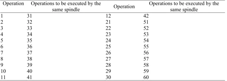
Precedence constraints, exclusion constraints for machining modules, turrets and working positions are presented in Tables 2, 3, 4 and 5, respectively. Inclusion constraints for machining modules are given in Table 6. Operations to be executed by the same spindle are presented in Table 7.
Table 2. Precedence constraints
Operation Predecessors Oper
ation Predecessors 2 1 3 31 33 40 5 7 9 11 35 37 39 41 4 1 3 31 33 42 9 11 39 41 6 5 7 9 35 37 39 44 43 45 8 5 7 9 35 37 39 46 43 45 10 5 7 9 11 35 37 39 41 48 47 49 12 9 11 39 41 50 47 49 14 13 15 17 19 52 21 51 16 13 15 17 19 53 22 52 18 13 15 17 19 54 23 53 20 13 15 17 19 62 61 63 22 21 51 64 61 63 23 22 52 66 65 67 24 23 53 68 65 67 32 1 3 31 33 70 69 71 73 75 34 1 3 31 33 72 69 71 73 75 36 5 7 9 35 37 39 74 69 71 73 75 38 5 7 9 35 37 39 76 69 71 73 75
Table 3. Incompatibility of operations in machining modules
Op Incom Op Incom Op Incom Op Incom
2 1 23 21 22 43 1-12, 31-42=* 63 25-30, 55-60 4 3 24 21-23 44 1-12, 31-42, 43 64 63 6 5 25-30 1 3 21-24 45 1-12, 31-42 66 65 8 7 31 2 13-20 25-30 46 1-12, 31-42, 45 68 67 10 9 32 1 13-20 31 47 1-12, 31-42 69 61-68 12 11 33 4 13-20 25-30 48 1-12, 31-42, 47 70 61-69 13 1-12 34 3 13-20 33 49 1-12, 31-42 71 61-68 14 1-13 35 6 13-20 50 1-12, 31-42, 49 72 61-68 71 15 1-12 36 5 13-20 35 51 22-30 73 61-68 16 1-12 15 37 8 13-20 52 21 23-30 51 74 61-68 73 17 1-12 38 7 13-20 37 53 21 22 24-30 51 52 75 61-68 18 1-12 17 39 10 13-20 54 21-23 25-30, 51-53 76 61-68 75 19 1-12 40 9 13-20 39 55-60 1 3 21-24 31 33 51-54 77 78 1 3 13 15 17 19 31 33 43 45 47 49 61 63=** 20 1-12 19 41 12-20 61 25-30, 55-60 79 **, 77 22 21 42 11 13-20 41 62 61 80 **, 78
Table 4. Incompatibility of operations in turrets
Operations Incompatible operations
13-20 1-12 25-30 21-24 31-42 13-20 43-50 1-12, 31-42 51-54 25-30 55-60 21-24, 51-54 69-76 61-68 77-80 21 51
Table 5. Incompatibility of operations in working positions
Operations Incompatible operations
21 1-20 25-30 1 3 21 31 21-30 32 21 33 21-30 34-50 21 51 1-20, 25-50 55-60 1 3 21 31 33 51 61 63 25-30 55-60 69-76 21 51 77-80 1 3 13 15 17 19 31 33 43 45 47 49 61 63
Table 6. Operations to be assigned to the same machining module Operation Operations to be in the same
machining module Operation
Operations to be in the same machining module 1 3 40 42 5 7 9 43 45 6 8 10 47 49 13 15 17 19 61 63 35 37 65 67 36 38 66 68 39 41 69 71 73 75
Table 7. Operations to be executed by the same spindle Operation Operations to be executed by the
same spindle Operation
Operations to be executed by the same spindle 1 31 12 42 2 32 21 51 3 33 22 52 4 34 23 53 5 35 24 54 6 36 25 55 7 37 26 56 8 38 27 57 9 39 28 58 10 40 29 59 11 41 30 60
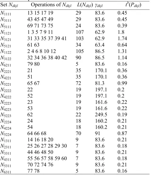
The total number of feasible orientations of all the parts was reduced to 16 due to the inclusion constraints (Table 7). The academic version of solver CPLEX 12.2 was used to solve the corresponding problems (1) – (41) for each combination of part orientations, but only one combination of part orientations resulted in a feasible system configuration. The obtained results are presented in Table 8. This solution was found in 0.56 seconds. The unfeasibility of 14 problems was discovered in 0.33 seconds on average. However, for one problem, 1.2 seconds were necessary to prove the unfeasibility of the problem. The total solution time was 6.5 seconds. The number of variables in MIP models was equal to 864.
The obtained optimal solution and its characteristics are presented in Tables 8 and 9. The vertical spindle head is common for positions 1, 2 and 3. Parts 1, 3, 5 are machined at position 1, part 6 is machined at position 2, and all the parts are machined at position 3. At position 1, there is a horizontal turret with 2 machining units (the first one is used for parts 1, 3, 5 and the second one is used for parts 1, 3). At position 2, there is a horizontal turret with 4 machining units which are used for machining parts 2, 4, and 5. The total time T(P) is equal to 16(3.18+0.28+3.41+0.28)+(3.41+0.1)+(0.28+3.18)-(3.41+0.28)+12(2.54+0.31+0.94+2.54)+(0.94+2.54)+(0.94+0.26)-(0.94+2.54)= 194.84 min.
Table 8. An optimal solution
Set Ndkjl Operations of Ndkjl L(Ndkjl) γdkjl tb(Pdkjl) N1111 13 15 17 19 29 83.6 0.45 N3111 43 45 47 49 29 83.6 0.45 N5111 69 71 73 75 24 83.6 0.39 N1121 1 3 5 7 9 11 107 62.9 1.8 N3121 31 33 35 37 39 41 103 62.9 1.74 N5121 61 63 34 63.4 0.64 N1122 2 4 6 8 10 12 105 86.5 1.31 N3122 32 34 36 38 40 42 90 86.5 1.14 N6211 79 80 5 83.6 0.16 N2221 21 35 170.1 0.36 N4221 51 35 170.1 0.36 N5221 65 67 72 81.3 0.99 N2222 22 19 197.1 0.2 N4222 52 19 197.1 0.2 N2223 23 19 161.6 0.22 N4223 53 19 161.6 0.22 N5223 62 22 249.5 0.19 N2224 24 18 160.2 0.21 N4224 54 18 160.2 0.21 N5224 64 66 68 70 91 0.87 N1311 14 16 18 20 9 83.6 0.21 N2311 25 26 27 28 29 30 7 83.6 0.18 N3311 44 46 48 50 9 83.6 0.21 N4311 55 56 57 58 59 60 7 83.6 0.18 N5311 70 72 74 76 9 83.6 0.21 N6311 77 78 5 83.6 0.16
Table 9. Characteristics of the solution Position k tp(P1k) tp(P2k) tp(P3k) tp(P4k) tp(P5k) tp(P6k) 1 3.41 0.1 3.18 0.1 0.94 0.1 2 0.1 1.49 0.1 1.49 2.54 0.26 3 0.31 0.28 0.31 0.28 0.31 0.26 5. Experimental study
The purpose of this study is to evaluate the effectiveness of the proposed techniques. There were generated series of 100 test instances for batches of 4, 6, 8 and 10 parts . Their characteristics are presented in Table 10, where |N| is the number of operations, OSP is the order strength of precedence constraints, DM, DT, DP, SS, and SM are the densities of graphs GDM, GDT, GDP, GSS, and GSM respectively, LS is the sum of lengths of loading sequences, NF is the number of families. Constraints were generated using tools developed previously [5]. Experiments were carried out on ASUS notebook (1.86 Ghz, 4 Gb RAM) with academic version of CPLEX 12.2.
Table 10
Parameters of problems for 4 parts Parameters of problems |N| OSP DM DT DP SS SM m0+1 LS NF Minimal value 44 0.034 0.064 0.026 0 0.027 0 4 8 2 Maximal value 95 0.525 0.659 0.659 0.242 0.051 0.016 8 16 2 Average value 69 0.106 0.373 0.348 0.024 0.036 0.004 6 12 2 Parameters of problems for 6 parts
Parameters of problems |N| OSP DM DT DP SS SM m0+1 LS NF Minimal value 89 0.029 0.003 0.002 0 0.024 0 3 6 2 Maximal value 159 0.471 0.462 0.462 0.205 0.031 0.057 9 18 2 Average value 124 0.29 0.228 0.197 0.027 0.027 0.016 6 12 2 Parameters of problems for 8 parts
Parameters of problems |N| OSP DM DT DP SS SM m0+1 LS NF Minimal value 118 0.023 0.003 0.002 0 0.024 0 3 8 2 Maximal value 216 0.456 0.438 0.417 0.214 0.033 0.057 10 20 2 Average value 165 0.288 0.197 0.168 0.025 0.028 0.017 6 12 2 Parameters of problems for 10 parts
Parameters of problems |N| OSP DM DT DP SS SM m0+1 LS NF Minimal value 251 0.023 0.025 0.02 0 0.014 0 4 12 2 Maximal value 255 0.062 0.58 0.588 0.194 0.026 0.005 9 27 3 Average value 254 0.04 0.326 0.3 0.031 0.019 0.001 7 18 2.5
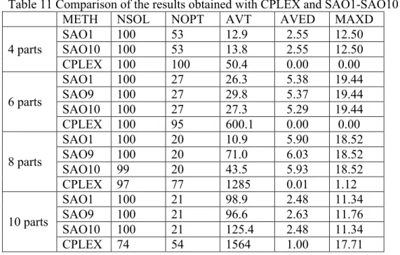
In Table 11 we compare results for CPLEX12.2 (maximal solution time 3600 sec) with SAO1 – SAO8 for TRnimp =500, Cmin = 0. TRtot was set to 1000 for SAO1 and SAO2 and 200 for SAO3-SAO8. Only the
best heuristic results are provided in Table 11. In this table NSOL is the number of problems with a founded feasible solution, NOPT is the number of problems with proven optimality, AVT is the average solution time (in sec), AVED and MAXD are average, and maximal deviations (in percents) of the found value of the objective function from the best known respectively. Minimal deviation was 0 for all instances.
Table 11 Comparison of the results obtained with CPLEX and SAO1-SAO10
METH NSOL NOPT AVT AVED MAXD
4 parts SAO1 100 53 12.9 2.55 12.50 SAO10 100 53 13.8 2.55 12.50 CPLEX 100 100 50.4 0.00 0.00 6 parts SAO1 100 27 26.3 5.38 19.44 SAO9 100 27 29.8 5.37 19.44 SAO10 100 27 27.3 5.29 19.44 CPLEX 100 95 600.1 0.00 0.00 8 parts SAO1 100 20 10.9 5.90 18.52 SAO9 100 20 71.0 6.03 18.52 SAO10 99 20 43.5 5.93 18.52 CPLEX 97 77 1285 0.01 1.12 10 parts SAO1 100 21 98.9 2.48 11.34 SAO9 100 21 96.6 2.63 11.76 SAO10 100 21 125.4 2.48 11.34 CPLEX 74 54 1564 1.00 17.71
These results show that the CPLEX solutions remain time-efficient for the problems with up to 6 different parts. For the problems with more parts to be produced, the heuristics can be used in the cases where CPLEX does not provide optimal solution or any solution at all. It can be noted that MAXD is superior for CPLEX solutions (a feasible solution found but not optimal) than for heuristic solutions. As a conclusion, both developed approaches are usefull in practice to treat different industrial cases.
5 Conclusion
The use of reconfigurable machining equipment can be an efficient response to increasing global competition and unpredictable market changes. Due to the physical structure that can be easily changed, the machining configuration can be optimized for each particular part family. The use of the optimization methods at this stage helps to reduce the total design time and to promptly discard unfeasible solutions. This paper proposed a decision support approach for the design of reconfigurable rotary machining systems with turrets used for producing several families of parts. The complex design constraints such as
compatibility and productivity requirements as well as design objectives were modeled within a mixed integer program. The model allows taking efficient decisions about part orientations, selection of machining modules and configuration/reconfiguration of working positions depending on the part families to be produced. The approach was validated on industrial case studies and one of these industrial examples was illustrated in the paper. The conducted study showed that the solution time to find the best cost-efficient machine configuration respecting all given constraints remains acceptable for the machine designers. Further development will concern the design of reconfigurable machining lines consisting of several reconfigurable machines. In order to evaluate the dynamic behaviour of the system, further studies should be conducted in order to develop appropriate simulation models and the integration scheme to combine optimization and simulation techniques in an efficient design scheme.
REFERENCES
[1] Abbasi, M., Houshmand, M. (2011) Production planning and performance optimization of reconfigurable manufacturing systems using genetic algorithm. International Journal of Advanced Manufacturing Technology, 54(1–4), 373-392.
[2] Agrawal, T., Sao, A., Fernandes, K.J., Tiwari, M.K., Kim, D. Y. (2013) A hybrid model of component sharing and platform modularity for optimal product family design, International Journal of Production Research, 51(2), 614-625.
[3] Battaïa, O., Brissaud, D., Dolgui, A., Guschinsky, N. (2015) Variety-oriented design of rotary production systems. CIRP Annals - Manufacturing Technology, 64(1), 411-414.
[4] Battaïa, O., Dolgui, A., Guschinsky, N., Levin, G. (2014) Integrated configurable equipment selection and line balancing for mass production with serial–parallel machining systems. Engineering Optimisation, 46(10), 2014, 1369-1388.
[5] Battaïa, O., Dolgui, A., Guschinsky, N., Levin, G. (2012) A decision support system for design of mass production machining lines composed of stations with rotary or mobile table. Robotics and Computer-Integrated Manufacturing, 28, 672-680.
[6] Battaïa, O., Dolgui, A., Guschinsky, N., Levin, G. (2012) Optimal design of machines processing pipeline parts. International Journal of Advanced Manufacturing Technology, 63, 963-973.
[7] Battaïa, O., Dolgui, A., Guschinsky, N., Levin, G. (2014) Combinatorial techniques to optimally customize an automated production line with rotary transfer and turrets. IIE Trasactions,46, 867-879.
[8] Bensmaine, A., Dahane M., Benyoucef. L. (2014) A new heuristic for integrated process planning and scheduling in reconfigurable manufacturing systems, International Journal of Production Research, 52(12), 3583-3594.
[9] Bi, Z. M., Lang, S. Y. T., Shen, W., Wang, L. (2008) Reconfigurable manufacturing systems: the state of the art, International Journal of Production Research, 46(4), 967-992.
[10] Borisovsky, P. A., Delorme X., Dolgui A. (2014) Balancing reconfigurable machining lines via a set partitioning model, International Journal of Production Research, 52(13), 4026-4036.
[11] Dou, J., Dai, X., Meng, Z. (2010) Optimisation for multi-part flow-line configuration of reconfigurable manufacturing system using GA. International Journal of Production Research, 48(14), 4071–4100.
[12] ElMaraghy H.A., Schuh G., ElMaraghy W., Piller F., Schönsleben P., Tseng M., Bernard A. (2013) Product Variety Management. CIRP Annals – Manufacturing Technology, 62, 629–652.
[13] Essafi, M., Delorme, X., Dolgui, A. (2012) A reactive GRASP and Path Relinking for balancing reconfigurable transfer lines, International Journal of Production Research, 50(18), 5213-5238.
[14] Goyal, K. K., Jain P.K., Jain, M. (2012) Optimal configuration selection for reconfigurable manufacturing system using NSGA II and TOPSIS, International Journal of Production Research, 50, 4175-4191.
[15] Goyal, K. K., Jain P.K., Jain, M. (2013) A comprehensive approach to operation sequence similarity based part family formation in the reconfigurable manufacturing system, International Journal of Production Research, 51 (6), 1762-1776
[16] Gumasta, K., Gupta, S.K., Benyoucef L., Tiwari M.K. (2011) Developing a reconfigurability index using multi-attribute utility theory. International Journal of Production Research, 49(6), 1669-1683. [17] Guschinskaya, O., Dolgui, A., Guschinsky, N., Levin, G. (2009) Minimizing makespan for multi-spindle head machines with a mobile table. Computers and Operations Research, 36 (2), 344–357.
[18] Gwangwava, N., Mpofu , K., Tlale, N., Yu, Y. (2014) A methodology for design and reconfiguration of reconfigurable bending press machines (RBPMs), International Journal of Production Research, 52(20), 6019-6032.
[19] Koren Y. (2013) The Rapid Responsiveness of RMS. International Journal of Production Research, 51(23–24), 6817–6827.
[20] Koren Y., Heisel U., Jovane F., Moriwaki T., Pritschow G., Ulsoy G., Van Brussel H. (1999) Reconfigurable Manufacturing Systems. CIRP Annals – Manufacturing Technology, 48(2), 527–540.
[21] Koren, Y., Shpitalni, M. 2010 Design of reconfigurable manufacturing systems. Journal of Manufacturing Systems, 29(4), 130-141.
[22] Koren, Y., Wang, W., Gu, X. (2016) Value creation through design for scalability of reconfigurable manufacturing systems, International Journal of Production Research, In Press.
[23] Kristianto, Y.; Gunasekaran, A. & Jiao, J. (2014) Logical reconfiguration of reconfigurable manufacturing systems with stream of variations modelling: a stochastic two-stage programming and shortest path model, International Journal of Production Research, 52, 1401-1418
[24] Liu, W., Liang, M. (2008) Multi-objective design optimization of reconfigurable machine tools: a modified fuzzy-Chebyshev programming approach, International Journal of Production Research, 46(6), 1587-1618.
[25] Makssoud, F., Battaïa, O., Dolgui, A. (2014) An exact optimization approach for a transfer line reconfiguration problem. International Journal of Advanced Manufacturing Technology 72, 717-727. [26] Mpofu, M. K., Tlale N. (2014) A morphology proposal in commercial-off-the-shelf reconfigurable machine tools, International Journal of Production Research, 52(15), 4440-4455.
[27] Renzi, C., Leali, F., Cavazzuti, M., Andrisano, A. O. (2014) A review on artificial intelligence applications to the optimal design of dedicated and reconfigurable manufacturing systems, International Journal of Advanced Manufacturing Technology, 72(1-4), 403-418.
[28] Saxena, L.K., Jain, P.K. (2012) A model and optimisation approach for reconfigurable manufacturing system configuration design, International Journal of Production Research, 50(12), 3359-3381.
[29] Singh, R. K., Khilwani, N., Tiwari, M. K. (2007) Justification for the selection of a reconfigurable manufacturing system: a fuzzy analytical hierarchy based approach. International Journal of Production Research, 45(14), 3165-3190.
[30] Tolio T., Urgo M. (2013) Design of flexible transfer lines: A case-based reconfiguration cost assessment. Journal of Manufacturing Systems, 32(2), 325-334.