Dynamic Shapes Average

HAL Id: inria-00608077

https://hal.inria.fr/inria-00608077

Submitted on 12 Jul 2011

HAL is a multi-disciplinary open access

archive for the deposit and dissemination of

sci-entific research documents, whether they are

pub-lished or not. The documents may come from

teaching and research institutions in France or

abroad, or from public or private research centers.

L’archive ouverte pluridisciplinaire HAL, est

destinée au dépôt et à la diffusion de documents

scientifiques de niveau recherche, publiés ou non,

émanant des établissements d’enseignement et de

recherche français ou étrangers, des laboratoires

publics ou privés.

Dynamic Shapes Average

Pierre Maurel, Guillermo Sapiro

To cite this version:

Pierre Maurel, Guillermo Sapiro. Dynamic Shapes Average. IEEE Workshop on Variational and

Level-Sets Methods in Computer Vision, Oct 2003, Nice, France. �inria-00608077�

Dynamic Shapes Average

Pierre Maurel

´

Ecole Normale Sup´erieure

75005 Paris, France

[email protected]

Guillermo Sapiro

Electrical and Computer Engineering

University of Minnesota

Minneapolis, MN 55455

[email protected]

Abstract

A framework for computing shape statistics in general, and average in particular, for dynamic shapes is introduced in this paper. Given a metric d(·, ·) on the set of static shapes, the empirical mean of N static shapes,C1, . . . , CN,

is defined by arg min_CN1 PN

i=1d(C, Ci)2. The purpose of

this paper is to extend this shape average work to the case of N dynamic shapes and to give an efficient algorithm to compute it. The key concept is to combine the static shape statistics approach with a time-alignment step. To align the time scale while performing the shape average we use

dy-namic time warping, adapted to deal with dydy-namic shapes.

The proposed technique is independent of the particular choice of the shape metric d(·, ·). We present the underlying concepts, a number of examples, and conclude with a vari-ational formulation to address the dynamic shape average problem. We also demonstrate how to use these results for comparing different types of dynamics. Although only aver-age is addressed in this paper, other shape statistics can be similarly obtained following the framework here proposed.

1. Introduction

Understanding shape and its basic empirical statistics is important both in recognition and analysis, with applica-tions ranging from medicine to security to consumer pho-tography. The basic metrics and statistics of static shapes have been the subject of numerous fundamental studies in recent years, see for example [1, 3, 4, 6, 8, 13, 15, 16] and

∗_{PM performed this work while visiting the University of Minnesota.}

We thank Renaud Keriven and Olivier Faugeras for suggesting and en-couraging this visit. We thank Facundo M´emoli, Alvaro Pardo, Renaud Keriven, Olivier Faugeras, and Paul Thompson for interesting discussions on shape statistics. This work was supported by a grant from the Office of Naval Research ONR-N00014-97-1-0509, the Presidential Early Career Award for Scientists and Engineers (PECASE), and a National Science Foundation CAREER Award.

references therein. In particular, given a metric on the set of static shapes (distance between two samples), the empirical mean shape of N static shapes, as well as other basic statis-tics, can be defined and computed. These are then used for diverse shape studies, from the recognition of particular ob-jects to the detection of abnormalities in medical data. The purpose of this work is to extend this to dynamic shapes. This is fundamental for studies such as those involving gait, behavior, growth patterns, and all problems involving mo-tion, deformations, and time-varying shapes.

Given N dynamic shapes Γ1(t), . . . , ΓN(t) (t stands for the time parameter, see Figure 1), we want to find M (t), the empirical mean of these shapes. This basic computation will be used throughout this paper as an example of how to perform statistics on dynamic shapes. One idea could be to simply perform static average among Γ1(t1), . . . , ΓN(t1), for each time instance t1, process that is clearly not effi-cient for every king of data. Indeed, the initial shape se-ries might not be time-aligned (e.g., due to different growth rates in medical applications and different motion speeds in gait analysis). The dynamic shapes need to be properly aligned before any kind of shape statistics technique is ap-plied.1This is exactly the role of the dynamic time warping (DTW), see Figure 1. This process is commonly used in speech recognition in order to time-align speech patterns to account for differences in speaking rates across speakers. It has also been used by a number of authors for gait analysis, but limited to the 1D path obtained by the tracking of partic-ular joints. In this work we propose to combine DTW with results on static shape analysis to compute basic statistics on dynamic shapes. The framework here proposed is inde-pendent of the particular choice of static shape metric. This work deals with discrete time instances, while the extension to a continuous framework is discussed in the conclusions section.

1_{The topic of time alignment appears also in video (see for example}

[2] and references in there). The goals and techniques used there are com-pletely different from the ones here presented. The use of our proposed framework for video alignment is the subject of future research.

2. Static Shape Averaging

In order to compute the mean of N static shapes, a dis-tance on the set of the shapes is necessary (for examples of such metrics see [3, 7, 13, 14] and references therein). Once the metric is given, the empirical mean shape can be defined:

Definition 1 Let d(·, ·) be a distance on the set of shapes

and C1, . . . , CN, N static shapes. The empirical mean M (C1, . . . , CN) is given by M (C1, . . . , CN) , arg min C N X i=1 d(C, Ci)2

The goal of this paper is to present a natural and easy to compute extension of this definition for dynamic shapes. Before doing this, let us briefly recall the second fundamen-tal component of our approach, dynamic time warping.

3. Dynamic Time Warping

Dynamic time warping (DTW) is principally used in speech recognition to time-align speech patterns in order to account for differences in speaking rates across speakers. A distance between two speech patterns can then be com-puted by this technique in order to be able to compare them (see [9]). DTW can be adapted to deal with other types of signals as done in this paper for shapes.

When the two signals (A, B) to be matched are de-fined as sampled time functions, A = a1, . . . , aL; B = b1, . . . , bM, the basic problem in DTW is to find two time

warping functions f and g such that

T X t=1

d(af (t), bg(t))2

is minimized (here d(·, ·) stands for the function measuring the discrepancy between two samples).

Computing these warping functions can be viewed as the process of finding a minimum-cost path through the lattice of points (ai, bj)(i,j)∈{1,...,L}×{1,...,M }, starting from (1, 1) and ending at (L, M ) (see Figure 2),2 _{where the cost of a} path is defined by:

D(f, g) , T X t=1

d(af (t), bg(t))2

and f and g are subject to the following constraints:

2_{Note that we use a}

iand biboth to denote the time positions and their

corresponding values, the distinction clearly provided by the context.

1. f and g must be monotonic:

f (k) ≥ f (k − 1) and g(k) ≥ g(k − 1) 2. f and g must match the endpoints of A and B:

f (1) = g(1) = 1, f (T ) = L and g(T ) = M 3. f and g must not skip any points:

f (k) − f (k − 1) ≤ 1 and g(k) − g(k − 1) ≤ 1 4. A limit in the maximum amount of warp is fixed by

|f (k)−g(k)| ≤ Q, Q being the given “window width” In the example in Figure 2, the time warping functions are:

f : 1 → 1, 2 → 2, 3 → 3, 4 → 4 5 → 5, 6 → 6, 7 → 6, 8 → 6 g : 1 → 1, 2 → 2, 3 → 2, 4 → 2 5 → 3, 6 → 4, 7 → 5, 8 → 6

At first glance, it would seem as if D(f, g) would have to be evaluated for a prohibitively large number of possible paths. Fortunately, dynamic programming brings this prob-lem under control by noting that the best path from (1, 1) to any given point is independent of what happens beyond that point. Hence, if we call D(ik, jk) the total cost of the best path from (1, 1) to (ik, jk), this is the cost of the point (ik, jk) itself plus the cost of the cheapest path to it:

D(ik, jk) = d(ik, jk)2+ min legal(ik−1,jk−1)

D(ik−1, jk−1) By the subscript “legal (ik−1, jk−1)” we mean the mini-mum over all permissible predecessors of (ik, jk). By con-straints 1 and 3 above, there are only three legal predeces-sors: (ik−1, jk), (ik, jk−1) and (ik−1, jk−1). Therefore we need to consider only three possibilities per lattice point (this if further constrained by point 4 above).

Dynamic programming for solving the DTW problem (finding f and g) then proceeds in incremental stages (see [9] for the complete algorithm), achieving an optimal time complexity of O(P Q) (P is the number of initial frames and Q the “window width” from constraint 4). It means that we need to compute d(·, ·), the distance between two static shapes, only O(P Q) times.

4. Dynamic Shapes Averaging

With the basic concepts on the mean of static shapes and dynamic time warping, we are now ready to describe the framework for dynamic shape average.

4.1

Basic Idea

We first define a dynamic shape as a sequence of static shapes (represented by any possible characterization):

Definition 2 Let S be a set of static shapes (using any

ex-isting representation). A dynamic shape Γ is an ordered sequence of static shapes (C1, . . . , CT) ∈ ST (T ∈ N is

the length of the dynamic shape).

Although the above definition is given for discrete times, it can be extended to continuous space.

The idea now is to combine dynamic time warping and static shape averaging:

Definition 3 Given d(·, ·), a distance on the set of static

shapes, and Γ1(t1), . . . , ΓN(tN), N dynamic shapes of

re-spective length Ti (i.e. ti = 1, . . . , Ti), their empirical

mean is defined as

for 1 ≤ t ≤ T : b_{Γ(t) , M (Γ}1(f1(t)), . . . , ΓN(fN(t)))

where f1, . . . , fN are N time-warping functions given by

(f1, . . . , fN) = arg min f1,...,fN T X t=0 µ(Γ1(f1(t)), . . . , ΓN(fN(t))) with µ(C1, . . . , CN) = X 1≤i<j≤N d(Ci, Cj),

and M (C1, . . . , CN) is the mean of static shapes (see

Def.1).

In words, we start by finding (via DTW) optimal time-correspondences between static shapes and after that we compute the average of these static shapes per time instance. The warping is such that the metric is minimized.

This definition suggests to consider the “distance” be-tween two dynamic shapes as follows (there is no triangle inequality here):

Definition 4 Given two dynamic shapes Γ1 and Γ2, their

“distance” is given by δ(Γ1, Γ2) = 1 T T X t=0 d(Γ1(f1(t)), Γ2(f2(t))),

where d(·, ·) is the selected metric for static shapes and f1

and f2are the optimal time warping functions.

This definition will be used later to compare human mo-tions.

4.2

Basic Improvements

With the simple use of DTW, the mean shape’s length T will be greater than or equal to the maximum of the indi-vidual time lengths {T1, . . . , TN}. Therefore, the dynamic mean shape will always be longer than the initial shapes (in Figure 2, T1= 6, T2= 6, T = 8). In order to correct this, we add jumps in the final path.

When N = 2, define, for i ∈ {1, 2},

Ei,{(bΓ(t), bΓ(t + 1)) | fi(t) = fi(t + 1)} where bΓ(·) is the dynamic mean shape (from Definition 3). E1 is the set of vertical segments and E2 the set of hor-izontal segments in the graph representing the final path. In Figure 2, E1 = {(bΓ(6), bΓ(7)), (bΓ(7), bΓ(8))} and E2 = {(bΓ(2), bΓ(3)), (bΓ(3), bΓ(4))}. These segments are responsi-ble for the increase of the final length. Indeed, we have the simple relation (T is the length of the mean shape without jumps) :

T = T1+ |E1| = T2+ |E2|

We opt to replace every second pair in E1by its static aver-age , then we do the same for the pairs in E2(see Figure 3). Each replacement decreases the length by one.

Therefore T’, the length of the mean shape with the jumps, becomes: T0= T −|E1| 2 − |E2| 2 = T1+ |E1| − |E2| 2 T0 = T1+ T2− T1 2 = T2+ T1 2

The length of the final mean shape is then the average of the length of the two initial shapes.

In the general case (N dynamic shapes), it is also intu-itive that we would like the length of the final mean shape to equal the average of the lengths of the N initial dynamic shapes. Therefore we now generalize the pairing process described above. Define, for any A ⊂ {1, . . . , N }:

EA,{(bΓ(t), bΓ(t + 1)) | fi(t) = fi(t + 1) ⇐⇒ i ∈ A} and, for any i ∈ {1, . . . , N }:

Ai,{A ⊂ {1, . . . , N } | i ∈ A}

Then the following relations, where T is the length of the mean shape without jumps, hold for any i ∈ {1, . . . , N } :

T = Ti+ X A∈Ai |EA| and T − 1 N N X i=1 Ti= 1 N X A⊂{1,...,N } |A| · |EA|

The right hand term of the previous equality can be elim-inated by the following process: For every subset A of {1, . . . , N }, we choose a number |A|·|EA|

N of pairs belong-ing to EA.3 Then we replace each pair by their static aver-age.The length of the final mean shape is then the average of the length of the N initial shapes. Figure 4 shows the mean shape for simple initial shapes and for N = 3.

5. Examples

For our experiments,we represented a static shape C by its distance function ψ(x) = miny∈Ckx − yk and we used the following simple metric on the set of static shapes:

d(C1, C2) = s

Z

Ω

(ψ1(ω) − ψ2(ω))2dω

where ψi(x) is the distance function to the shape Ci. For this distance, bC, the average shape, is the zero level set of

b ψ(x) = 1

2(ψ1(x) + ψ2(x))

As mentioned in the introduction, the framework here introduced is independent of the particular choice of the static metric d(·, ·), and we have selected this simple one for demonstration purposes only.

The segmentation of the input pictures is done by sim-ple thresholding ([12, 10]), and the distance function ψifor each shape Ci is computed with the fast marching method (for details, see [5, 11, 17]). Figure 5 shows an example (one frame) of an initial dynamic shape.

In figures 6 and 8, we present a number of frames from two initial video clips (dynamic shapes), followed by sam-pled frames from the average dynamic shape computed without using DTW, and finally sampled frames from the average dynamic shape computed with our technique. Fig-ures 7 and 9 show the corresponding DTW graphs.

In Figure 10, we present some frames from three ini-tial video clips (three walking men), followed by sampled frames from the mean dynamic shape computed without us-ing DTW, and finally with our technique.

Using Definition 4, we can compare different dynamics, such as running vs. walking men. As observed in the table below, this function is five times greater between one run-ning men and one walking men than between two runrun-ning or two walking men.

δ(·, ·)/106 walk 1 walk 2 run 1 run 2

walk 1 0 1.3 5.6 6.3

walk 2 1.3 0 5.2 6.7

run 1 5.6 5.2 0 1.1

run 2 6.3 6.7 1.1 0

3_{We choose these pairs uniformly spread in time.}

6. Conclusion

A novel framework for performing shape statistics in dy-namic shapes was described in this paper. The basic idea is to combine shape alignment with previously developed ideas from static shape studies. The shape alignment is based on dynamic time warping. The framework is inde-pendent of the metric between static shapes.

A number of directions are suggested by the line of re-search here initiated. First of all, other more advanced static shape metrics need to be used, including those that incorpo-rate landmarks, found to be fundamental for medical appli-cations [15]. Once these advanced metrics are incorporated into our framework, we can proceed with more exhaustive experimentation, including 3D dynamic shapes. Of partic-ular interest are the analysis and recognition of gait and the study of growth in medical applications.

In this paper we limited ourselves to the case of discrete time. In the continuous case, a variational formulation to address the dynamic shape average problem can be formu-lated as arg min Γ,fi Z T 0 X 1≤i≤N [d(Γ(t), Γi(fi(t))2 + H(fi(t)]dt

where fi are the time warping functions, and H represents some constraints on them (such as continuity, monotonicity, acceleration, etc). To this we can add time domain land-marks (e.g., by splitting the domain). These topics are the subject of current efforts in our group.

References

[1] F. Bookstein. Size and shape spaces for landmark data in two dimensions. Statistical Science, 1:181–242, 1986. [2] Y. Caspi and M. Irani. Parametric sequence-to-sequence

alignment. IEEE Transactions on Pattern Analysis and Ma-chine Intelligence.

[3] G. Charpiat, O. Faugeras, and R. Keriven. Approximations of shape metrics and application to shape warping and em-pirical shape statistics. Technical report, INRIA–RR-4820, 2003.

[4] T. Cootes, C. Taylor, D. Cooper, and J. Graham. Active shape models: Their training and application. Computer Vi-sion and Image Understanding, 61(1):38–95, 1995. [5] J. Helmsen, E. G. Puckett, P. Collela, , and M. Dorr. Two

new methods for simulating photolithography development in 3d. Proc. SPIE Microlithography, IX:253, 1996. [6] I. L. IDryden and K. V. Mardia. Statistical Shape Analysis.

John Wiley & Sons, New York, 1998.

[7] D. G. Kendall. Shape manifolds, procrustean metrics and complex projective spaces. Bulletin of the London Mathe-matical Society, 16:81–121, 1984.

[8] M. Miller and L. Younes. Groups actions, homeomorphisms and matching: A general framework. International Journal of Computer Vision, 41(1/2):61–84, 2001.

[9] T. Parsons. Voice and Speech Processing. McGraw-Hill, 1987.

[10] P. K. Sahoo, S. Soltani, A. K. C. Wong, and Y. C. Chen. A survey of thresholding techniques. Computer Vision, Graph-ics, and Image Processing, 41(2):233–260, Feb. 1988. [11] J. A. Sethian. A fast marching level-set method for

monotonically advancing fronts. Proc. Nat. Acad. Sci., 93:4:1591–1595, 1996.

[12] L. G. Shapiro and G. C. Stockman. Computer Vision. Pren-tice Hall, 2001.

[13] C. G. Small. The Statistical Theory of Shape. Springer, 1996.

[14] S. Soatto and A. J. Yezzi. Deformotion: Deforming motion, shape average and the joint registration and approximation of structures in images. International Journal of Computer Vision, 53(2):153–167, 2003.

[15] A. Toga. Brain Warping. Academic Press, 1998.

[16] A. Trouv´e and L. Younes. Diffeomorphic matching prob-lems in one dimension: Designing and minimizing matching functionals. In ECCV’00, pages 573–587, 2000.

[17] J. N. Tsitsiklis. Efficient algorithms for globally opti-mal trajectories. IEEE Transactions on Automatic Control,

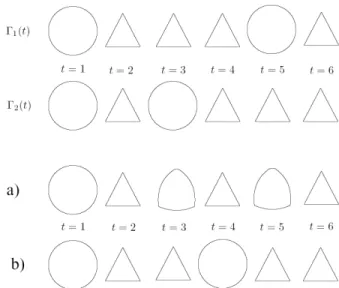
40:1528–1538, 1995. Figure 1. A simple example showing the

im-portance of time alignment when performing shape statistics. The first two rows show two dynamic shapesΓ1(t)andΓ2(t). The

fol-lowing two rows show their mean: a) Com-puted without DTW-alignment, b) ComCom-puted

with enhanced DTW-alignment. We clearly

observe the need for the DTW step.

Figure 3. Example of the introduction of jumps in DTW forN = 2.

Figure 4. Example of mean shape, with jumps, for simple initial shapes andN = 3.

Figure 5. From left to right: Initial image, seg-mented shape, and distance function

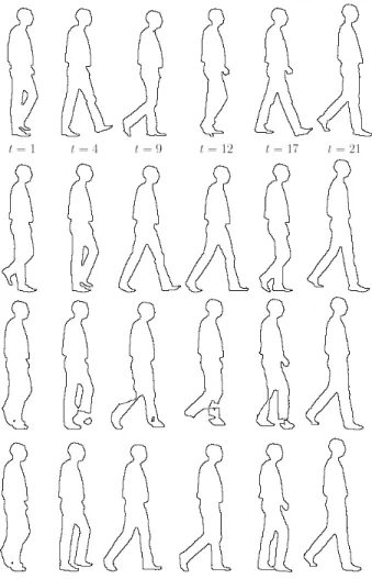
Figure 6. Example of two walking men. The two dynamic shapes are given first, followed by the mean without DTW (third row), and fi-nally the mean with DTW (last row). Note how the lack of time alignment creates topological errors, not present in the average when DTW is used.

Figure 7. Graph corresponding to the DTW for the running sequences.

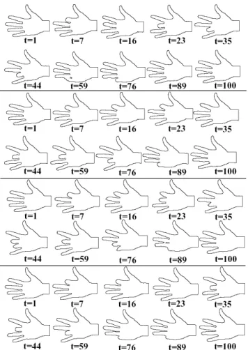
Figure 8. Same as Figure 6 for two hands in motion.

Figure 9. Graph corresponding to the DTW for the hands sequences.

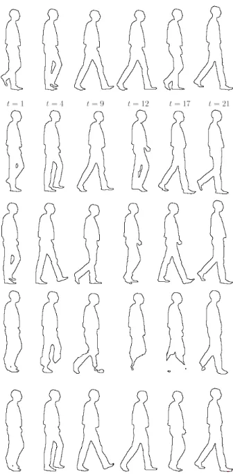
Figure 10. Example of three walking men. The three dynamic shapes are given first, followed by the mean without DTW (fourth row), and fi-nally the mean with DTW, our proposed tech-nique (last row). Once again, note the signif-icant improvement when the time-warping is added to the shape statistics process.