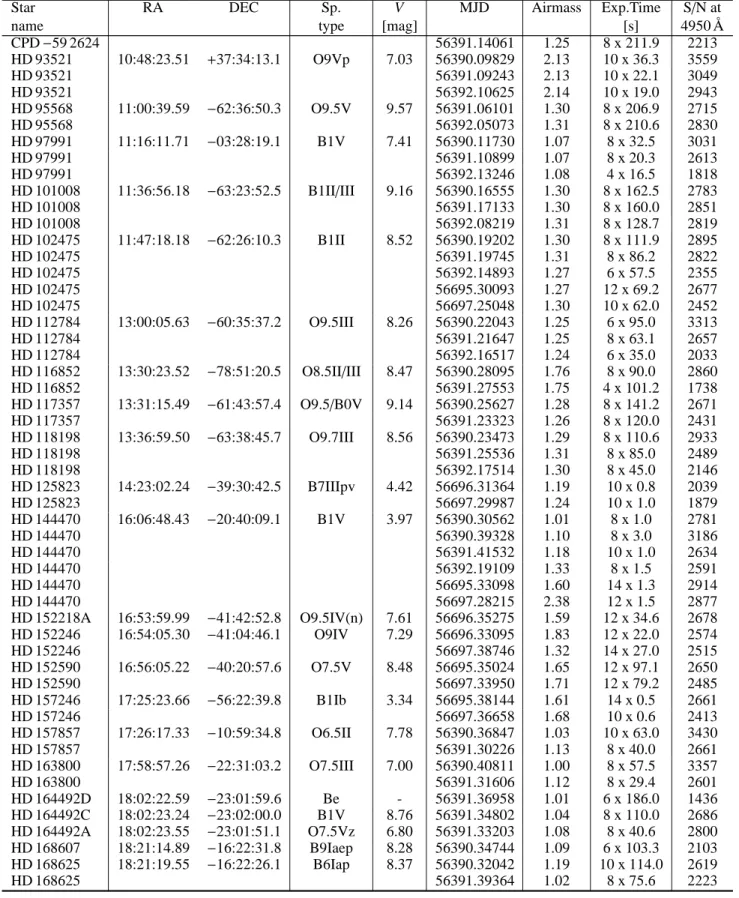
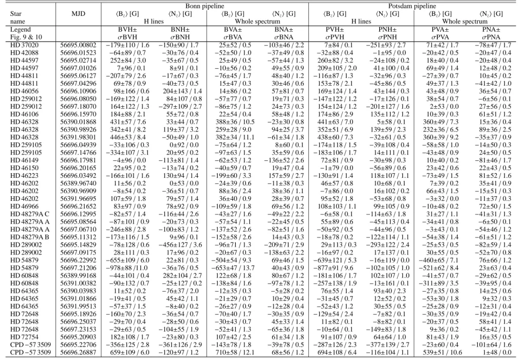
B fields in OB stars (BOB): low-resolution FORS2 spectropolarimetry of the first sample of 50 massive stars

When monitored on solid medium and thus without oxygen limitation, 68 and 77% of the tested strains were able to reduce nitrate and nitrite, respectively (Supplementary Figures

However, those images cover limited geographic areas and the evaluation procedure does not as- sess how the methods generalize to different contexts or more abstract semantic

"Development of European hydrogen infrastructure scenarios--CO2 reduction potential and infrastructure investment." Energy Policy Hydrogen 34(11), 1284-1298.

In an in-depth exploration of the synthesis of diblock copoly- mers 24, Sleiman developed a step-wise procedure: in the first step, the ruthenium catalyst induced polymerization of

Dans cette partie nous allons voir comment nous sommes passés d’un moyen de mesure manuel à une solution de test automatisé en examinant les deux points cruciaux qui

En este sentido, se observa que se subestima el potencial de Internet, la web y las redes sociales en relación a la promoción turística, ya que, aunque todos los museos entienden

The impact of each of the five parameters (energy, next-node distance, sink distance, node density, and message priority) utilised in the proposed MFWF was comparatively assessed

Le recensement exhaustif des admissions indique que parmi 263 jeunes admis avant 2000 (incluant des accueils en urgence, des placements courts et des réorientations avant la fin