Université de Montréal
Importance de la taille et du contexte spatial des unités d’analyse
sur la structure, le pouvoir prédictif et l’extrapolation des modèles de qualité d’habitat.
Par Mariane Fradette
Département de Sciences Biologiques faculté des Arts et des Sciences
Mémoire présenté à la Faculté des études supérieures en vue de l’obtention du grade de maîtrise en sciences biologiques.
Juin 2006
C
C
/,:
;
e-Université
de Montréal
Direction des bibliothèques
AVIS
L’auteur a autorisé l’Université de Montréal à reproduire et diffuser, en totalité ou en partie, par quelque moyen que ce soit et sur quelque support que ce soit, et exclusivement à des fins non lucratives d’enseignement et de recherche, des copies de ce mémoire ou de cette thèse.
L’auteur et les coauteurs le cas échéant conservent la propriété du droit d’auteur et des droits moraux qui protègent ce document. Ni la thèse ou le mémoire, ni des extraits substantiels de ce document, ne doivent être imprimés ou autrement reproduits sans l’autorisation de l’auteur.
Afin de se conformer à la Loi canadienne sur la protection des renseignements personnels, quelques formulaires secondaires, coordonnées ou signatures intégrées au texte ont pu être enlevés de ce document. Bien que cela ait pu affecter la pagination, il n’y a aucun contenu manquant. NOTICE
The author of thïs thesis or dissertation has granted a nonexclusive license allowing Université de Montréal to reproduce and publish the document, in part or in whole, and in any format, solely for noncommercial educational and research purposes.
The author and co-authors if applicable retain copyright ownership and moral rights in this document. Neither the whole thesis or dissertation, nor substantial extracts from it, may be printed or otherwise reproduced without the author’s permission.
In compliance with the Canadian Privacy Act some supporting forms, contact information or signatures may have been removed from the document. While this may affect the document page count, t does flot represent any loss of content from the document.
11
Université de Montréal Faculté des études supérieures
Ce mémoire intitulé
Importance de la taille et du contexte spatial des unités d’analyse
sur la structure, le pouvoir prédictif et l’extrapolation des modèles de qualité d’habitat.
Présenté par: Mariane Fradette
a été évalué par un jury composé des persoimes suivantes
Bemard Angers président-rapporteur Daniel Boisclair directeur de recherche Normand Bergeron membre du jury
111
RÉSUMÉ
Un modèle de qualité d’habitat met en relation un indicateur de la valeur écologique d’une série de sites d’échantillonnage pour une espèce ou une communauté (p résence/absence, densité, production, etc.) et les conditions environnementales caractérisant ces sites (pH, composition du substrat, production primaire, etc.). L’objectif de cette étude est de voir les effets de la taille et du contexte spatial des unités d’analyse sur la structure, le pouvoir prédictif et l’extrapolation des modèles de qualité d’habitat. Pour y arriver, nous avons échantillonné une section de 14.7 km de la Rivière Sainte-Marguerite (Région du Saguenay, Québec) de façon à obtenir des séries spatiales continues de la densité de juvéniles du saumon Atlantique ainsi que de différentes caractéristiques de l’environnement de nature locale (vitesse du courant, composition du substrat, etc.) ou de contexte spatial (distance à la plus proche frayère en amont, présence de remblaiements sur la berge, etc.). Nos résultats montrent que la taille des unités d’analyse influence la structure ainsi que le pouvoir prédictif des modèles. Les modèles développés avec des unités d’analyse provenant de la fusion d’unités d’échantillonnage similaires (taches d’habitat) ou avec des unités d’analyse dont la longueur est similaire à celle de ces taches (200 m dans notre étude) ont un meilleur pouvoir prédictif et une meilleure capacité d’extrapolation que les modèles développés avec de petites unités d’analyse. Bien que les variables locales restent essentielles lors d’une modélisation d’habitat, les variables de contexte spatial contribuent à augmenter le pouvoir prédictif des modèles.
iv
ABSTRACT
Habitat quality models are quantitative relationships between indicators of the ecological value of a series of sampling units (e.g. presence/absencc, density, growth, survival, production, etc) and the environrnental conditions prevailing at these units (e.g. temperature, substrate composition, pH, etc). The purpose ofthis study was to assess the effects of the size and the spatial context of analytical units on the structure, the predictive power, and the upscaling of habitat quality models. We sarnpled a 14.7 km section in the Sainte-Marguerite River (Saguenay region, Quebec) in a way to obtain continuous spatial series for juveniles Atiantic salmon density, and for different local habitat characteristics (flow velocity, substrate composition, etc.) and spatial context characteristics (distance to the nearest tributary upstream, presence of embankment in the shore, etc.). Our results are consistent with the expectation that changing the size of analytical units may affect the structure and the predictive ability of habitat quality models. Our analyses suggest that the merging of sampling units possessing similar environrnental conditions to form habitat patches or analytical units that have a size similar to habitat patches (i.e. in our study analytical units of 200 m) may improve the predictive ability and the upscaling of habitat quality models. Our study also indicates that, while local variables often explain most of the variation of indices of habitat quality, spatial context variables may also increase the predictive power of habitat quality models.
V
TABLE DES MATIÈRES
Page titre
Identification du jury ii
Résumé iii
Abstract iv
Table des matières y
Liste des tableaux vi
Liste des figures vii
Liste des abréviations ix
Dédicace x
Remerciements xi
introduction générale 1
Importance ofthe size and the spatial context ofanalytical units on the structure, the predictive power, and the upscaling
of habitat quality models $
Introduction 9 Methods 11 Resuits 27 Discussion 3$ Conclusion 43 Aknowlegments 44 Conclusion générale 45 Références bibliographiques 47
vi
LISTE DES TABLEAUX
Table 1. Environrncntal characteristics included as potential explanatory variables
in the
habitat quality models.
Table Il. Substrate size classes used in this study.
Table III. Average and variance (in parenthesis) of JAS density and selected environmental variables for each size ofanalyticat units (AU). HPÏ corresponds to the model developed with alt habitat patches, and HP2 corresponds to the moUd developed with habitat patches
> 50 m. ANOVAs and Levene tests that are statistically significant at the threshold of
p=O.05 are marked with an * in the “pAU” columii for the tests between AU sizes, and in the “pHP” colunm for the tests between AU sizes and HP models.
Table 1V. Habitat quality models that successfully predicted JAS density variations during the cross-validation exercise. Numbers in bold are partial R2adj.. Numbers in italic are the beta coefficients ofeach variable in the regression models.
vii
LISTE DES FIGURES
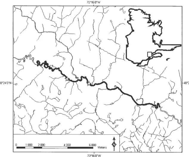
figure 1. Study area of 14.7 km on the Sainte-Marguerite River. White stars along the Sainte-Marguerite River represent beginnings ofsedimentary Iinks.
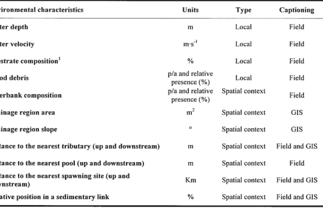
Figure 2. Substrate composition of habitat types determined by the K-means grouping method.
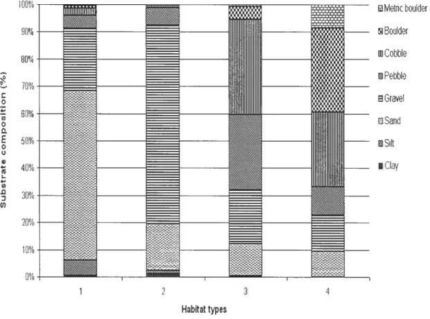
Figure 3. Frequency distribution ofthe size of habitat patches.
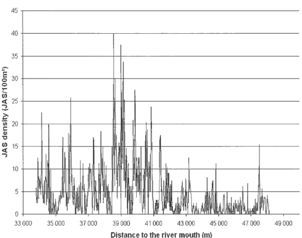
Figure 4. Spatial distribution of JAS density in the study area. The size of the sampling sections used to describe fish distribution in this figure is 20 m.
figure 5: Results of the bootstrap analysis. Bars represent 95% confidence intervals of R2adj for 1 000 iterations of models developed using different sizes of analytical units (AU). Squares represent original values ofR2adj..
Figure 6: Results of the cross-validation analysis. Bars represent 95% confidence intervals of r of Pearson of the relation between observed and predicted JAS density for 1 000 iterations of models developed using different sizes of analytical units (AU). Squares represent medians of r ofPearson.
Figure 7: Resuits of the cross-validation analysis. Bars represent 95% confidence intervals of the slope of the relation between observed and predicted JAS density for 1 000 iterations of models developed using different sizes of analytical units (AU). Squares represent medians ofslopes.
Figure 8: Results of the cross-validation analysis. Bars represent 95% confidence
viii 1 000 iterations of models devetoped using different sizes of analytical units (AU). Squares represent medians of intercepts.
ix
LISTE DES ABRÉVIATIONS
AU $ Analytical unit
Cl: Confidence interval HP : Habitat patch
HQM : Habitat quality model JAS : Juvenile Atiantic salmon
JSA : Juvénile du saumon de l’Atlantique MAUP : Modifiable areal unitproblem MQH : Modèle de qualité d’habitat R2adj. : Adjusted R2
SMR: Sainte-Marguerite River SU: Sampling tinit
UA : Unité d’analyse
X
Sornetirnes, there is just no way to hold back the river.
xi
REMERCiEMENTS
À
Daniel Boisclair. pour son optimisme. ses idées. son assiduité et sa patience.À
Judith Bouchard avec qui j’ai partagé totis les aspects de cette aventure dans te monde de la recherche scientifique. Sans toi Judith, je ne stiis vraiment pas sûre que
j
‘aurais réussià passer à travers... Aux gens qui m’ont aidé sur le terrain durant mes deux étés d’échantillonnage. Pour votre dévouement, votre rigueur et pour tous les chocolats chauds bus stir ta 172 (Nuwïts un jour, Nuwïts toujours!).
À
André Boivin, à Albertine, aux deux Collette, à Édith et à tous les gens du CIRSA. Ces étés passés parmi vous ont été tout simplement magiques.À
la gang du labo Boisclair, particulièrement à Guillaume Guénard pour son inconcevable connaissance des statistiques et du langage R.À
Philippe Girard qui ma beaucoup aidé avec mon introduction.À
tous les étudiants aux études gradués en biologie de l’Université de Montréal. Toutes ces personnes ont contribué, peut-être sans le savoir, à l’aboutissement de ce projet par leur soutien moral (surtout à l’occasion des très sérieuses réunions de l’AECBUM..-)
et par le partage de leur expérience personnelle.À
ma chère famille qui m’a permis de me rendre jusque là. Pour leur soutien sans faille et lettr amour réconfortant.À
mes merveilleuses amies. Je ne sais pas quoi vous dire d’autre que je vous aime! Je m’ennuie de vous! Venez toutes habiter à Riki!!À
mon amoureux que j’aime que j’aime que j’aime!À
Bruno et àMartinepour leur soutien involontaire mais très efficace.
INTRODUCTION
GÉNÉRALE
Uti habitat est constitué dun ensemble de facteurs physiques et biologiques qui permettent à un organisme vivant de subvenir à ses besoins (Barbour et al. 1999). Depuis environ 200 ans, la surpopulation humaine, la surexploitation des ressources
naturelles et la pollution ont entraîné une perte d’habitat pour de nombreuses espèces animales et végétales à l’échelle de la planète (Chiras et al. 2002). Selon le dernier rapport de l’Union internationale pour la conservation de la nature (IUCN; Baillie et al. 2004), la destruction, la dégradation et la fragmentation des habitats sont les plus grandes menaces pour les animaux terrestres, avec un impact sur 86 % des oiseaux et des mammifères menacés et sur $8 % des amphibiens menacés. La perte d’habitat est également la plus grande menace pour les espèces animales d’eaux douces et la deuxième plLts grande menace pour les espèces animales marines, après la surexploitation. Dans cet optique, il devient très important de développer des stratégies de conservation des habitats les moins altérés et d’élaborer des plans de restauration et d’aménagement pour les habitats endommagés.
Les écosystèmes sont des mosaïques complexes d’habitats présentant différentes conditions environnementales (Duiming et al. 1992). Cette hétérogénéité spatiale suggère que les différents habitats contribuent de façon non équivalente au maintien des populations et des communautés. Le modèle de qualité d’habitat (MQH) est un outil de synthèse qui s’avère très utile lorsqu’on cherche à représenter les relations entre des individus et leur environnement. Il existe plusieurs formes de MQH. Par exemple, les courbes de préférences montrent s’il y a des associations positives ou négatives d’une
espèce avec certaines caractéristiques de l’habitat en fonction de la disponibilité de ceux-ci (Guay et al. 2000; Crook et al. 2001). L’indice de qualité d’habitat classe les habitats sur un gradient de qualité pour une espèce ou une communauté selon différents facteurs physiques, chimiques ou biologiques associés à ces habitats (Courtois 1993; Guay et al 2000). Un autre indice, développé par Karr (1981) et qui s’applique plus particulièrement aux cours d’eau, permet d’évaluer les effets des perturbations anthropiques en milieu aquatique en évaluant l’intégrité des habitats en comparant les communautés ichtyologiques (ott d’invertébrés ou autres) des habitats perturbés avec celles des habitats non-perturbés (Rioux et Gagnon 2000). finalement, le modèle de régression met en relation un indice de la valeur écologique (ex production, biomasse, densité, taux de croissance, taux de survie, etc.) et des conditions environnementales (ex : pH, production primaire, présence de refuges,...) dans une série d’unités d’échantillonnage (liE; ex quadrats, parcelle, etc.). Ces modèles se présentent sous forme d’équation mathématique dont l’expression la plus simple est
y = bjxj+bx + b() [11
où y est l’indice de la valeur écologique à un UE, x1 et x2 sont des variables environnementales et b1, b2 et ho sont des constantes (Turgeon et Rodrigtiez 2005). Dans un but de conservation et d’aménagement, les MQH devraient idéalement permettre aux scientifiques et aux gestionnaires d’identifier les habitats possédant une grande valeur écologique pour une population ou une communauté dônnée et de prédire les effets de perturbations naturelles ou anthropiques sur les habitats (Gibson et al. 2004; Newbold et Eadie 2004; Woithon et Schmieder 2004; Bowman et Robitaille 2005; Klaus et al. 2005; VanManen et al. 2005).
3 L’étape finale du processus de modélisation est de transférer le modèle ayant été développé i partir d’observations faites sur un ensemble d’UE une autre portion de
l’écosystème où l’on souhaite identifier les habitats à haute valeur écologique. Cette extrapolation nécessite l’adoption de certaines prémisses. Cependant, les études de modélisation ne tiennent que rarement compte de celles-ci.
La première prémisse est que la taille des unités utilisées pour les analyses
statistiques menant au développement de MQH, les unités d’analyse (UA; dont ta taille peut différer de celle des UE, selon le design «échantillonnage; BrindArnour et Boisclair 2006) permet une description adéquate des processus écologiques de l’écosystème. Cependant, la taille des UE ou des UA est plus souvent déterminée par des contraintes logistiques (temps requis pour l’échantillonnage, distance entre les sites d’échantillonnage, etc.) que par des considérations écologiques. De plus, la taille des UA est reconnue pour affecter la structure, cest-à-dire les variables enviromwmentales incluses dans les modèles ainsi que le sens des relations entre celles-ci et l’indice de la valeur écologique, et le pouvoir prédictif des modèles empiriques (Wiens 1989; fotheringham et Wong 1991; Jelinski et Wu 1996; foIt et al. 1998). Ce phénomène, appelé problème des unités à aires variables, a été observé dans plusieurs études empiriques. Ce problème a, selon Jelinski et Wu (1996) deux composantes 1) le problème d’échelle, ou dépendance d’échelle, vient du fait qu’il est pôssible d’arriver à des résultats différents lorsque les mêmes données sont analysées à des échelles différentes. Par exemple, Bult et al. (199$) ont démontré que, à grandes échelles (>4 m), les juvéniles du saumon de l’Atlantique ($aÏmo saÏar) montrent une grande préférence pour les habitats peu profonds. Par contre, des analyses à une plus petite échelle (< 1m)
4 à l’intérieur de ces habitats montrent que les juvéniles sont plutôt associés à des micro-habitats d’eau profonde au sein des habitats d’eau peu profondes. Une autre étude (Crook et al. 2001) suggère qu’à l’échelle dti micro-habitat, la distribution de la perche dorée (Macqitaria ambigua) est positivement associée à la présence de débris ligneux,
tandis qu’à l’échelle du méso-habitat, cette association est négative. De plus, Brind’Amour et al. (2005) ont démontré qu’une communauté de poissons littoraux a une distribution spatiale structurée à plusieurs échelles et que les conditions environnementales influencent cette distribution de façon différente à toutes les échelles. 2) Le problème de zonage évoque le fait qu’une série d’UE combinées en UA qui ont la même surface mais qui sont positionnées différemment dans l’espace peut mener à des résultats différents à chaque analyse. Brind’Amour et Boisclair (2006) ont effectivement montré que, pour une communauté de poissons littoraux lacustres, te pourcentage de variance de l’indice de valeur écologique expliquée par les variables environnementales varie beaucoup pour des modèles développés avec des UA de même dimensions même avec des zonages différents.
La seconde prémisse est que les caractéristiques environnementales estimées dans une UA spécifique permettent une représentation adéquate de l’éventail complet des conditions affectant la qualité des habitat, non seulement de cette unité, mais de toutes les unités de l’écosystème étudié. Traditionnellement, les caractéristiques environnementales utilisées dans les MQH sont des caractéristiques locales décrivant le micro-habitat. Cependant, plusieurs études conceptuels (Schlosser 1991; Kocik et Ferreri 199$) et évaluations sur le terrain (Dunning et al. 1992; Schiosser 1995; Pess et al. 2002; Brind’Amour et Boisclair 2006) suggèrent que la qualité d’un habitat n’est pas
seulement reliée à ses attributs intrinsèques mais également à ce qu’il y a autour de lui. Ces caractéristiques environnementales, faisant référence au contexte spatial des UA, représentent les interactions pouvant exister entre des habitats plus ou moins éloignés.
Par exemple, Petit (1989) a bien illustré le phénomène de complémentarité en montrant qu’en hiver, les oiseaux forestiers n’utilisent pas les habitats d’alimentation qui ne sont pas situés à proximité d’un refuge contre le vent et la neige. Un autre concept, celui de la supplémentarité, fait référence à ta fragmentation des habitats dans ce sens où les individus vivant dans une tache d’habitat trop petite pour subvenir à un besoin en particulier doivent avoir la possibilité de se déplacer dans une autre tache d’habitat pour combler ce besoin. Whitcomb et al. (1977) ont décrit un cas de supplémentarité d’habitats en recensant les populations d’oiseaux de plusieurs boisés dans un paysage
fragmenté. Kocik et Ferrreri (199$) ont démontré l’importance de tenir compte du positionnement spatial des sites de fraie et des habitats d’alimentation dans une rivière pour estimer la production de juvéniles de saumon de l’Atlantique. Enfin, l’effet de voisinage est bien démontré dans une étude de Pess et al. (2002) qui montre que l’abondance de saumons coho (Oncorhynchus kisutch) dans la rivière Snohomish (Washington, É.-U.) est corrélée à la nature de l’utilisation des terres à proximité du cours d’eau.
Le saumon de l’Atlantique est tin bon exemple d’espèce pour laquelle les modèles traditionnels, qui ne tiennent pas compte des deux prémisses énoncées plus haut, ne parviennent pas à fournir des otttils réellement utiles pour sa conservation. Jusqu’à maintenant, la grande majorité des études de modélisation d’habitat des juvéniles du saumon de l’Atlantique (JSA) se sont limitées à utiliser des UE d’au plus
6
une centaine de mètres, ont fait des analyses avec une seule taille d’UA et ont employé des variables caractérisant l’habitat local des JSA, comme la vitesse du courant, la profondeur de l’eau ou la composition du substrat (Wankowski et Thorpe 1979; DeGraaf et Bain 1986; Morantz et al. 1987; Heggenes et al. 1990; Bourgeois et al. 1996; Gries et Juanes 1998; Guay et al. 2000; Bélanger et Rodrguez 2002; Mki-Petys et al. 2002; Hedger et al. 2004; Turgeon et Rodriguez 2005). foIt et al. (1998), qui ont fait une revue de littérature pour déterminer les échelles spatiales et temporelles utilisées dans la recherche sur le saumon de l’Atlantique, montrent que plus de 85% des études utilisent
plusieurs petites parcelles au sein d’une même rivière pour leurs analyses. De plus, ils remarquent que très peu d’études incluent plus d’une échelle dans leur analyses, ce qui permettrait de détecter les contradictions liés ati problème des unités à aires variables et de déterminer la taille optimale d’UA. Pour leur part, Armstrong et al. (2003) ont répertorié des études sur les habitats utilisés par les JSA et ont remarqué qu’il y avait de grandes différences entre les résultats des ces études qui utilisaient pourtant toutes les même variables locales pour caractériser les habitats. Seulement quelques études théoriques (Armstrong et al. 199$; Kocik et Ferreri 1998; Bardoimet et Baglinière 2000) ou empiriques (Bult et al. 1998; Poff et Huryn 1998) ont considéré qu’il était important de faire des analyses multi-échelle et de tenir compte d’autres variables environnementales que les variables traditionnelles locales lorsqu’on souhaite développer des MQH pour les JSA en rivière.
Le saumon de l’Atlantique est une espèce dont la majorité des populations
sauvages sont en déclin depuis les dernières décennies. Quelques unes ont même été
7 des clés du problème de conservation des populations sauvages de saumons de l’Atlantique. Premièrement, il est plus facile d’étudier et d’intervenir au niveau des cours d’eau que dans l’océan, où les coûts associés et les difficultés tecimiques sont accrus. De plus, les rivières sont des habitats cruciaux pour cette espèce puisque c’est là que les juvéniles vont naître et se développer (Poff et Nuryn 1998). Il est donc très important de bien coirnaître ces habitats pour ensuite élaborer des stratégies de conservation efficaces.
Le premier objectif de cette étude sera donc dévaluer comment la taille des AU influence le pouvoir prédictif et le pouvoir d’extrapolation des MQH pour les ISA en rivière. Nous croyons que les modèles développés avec différentes tailles d’UA auront des pouvoirs prédictifs et d’extrapolation différents, cependant, aucun indice dans la littérature ne 110L15 permet de prédire dans quel sens iront ces différences. Le dettxième
objectif sera d’évaluer les effets du contexte spatial des UA sur la structure et le pouvoir prédictif de ces MQH. Dans, ce cas-ci, nous croyons que des variables environnementales décrivant le contexte spatial des UA auront un rôle significatif à jouer lors du développement des MQH.
Pour rencontrer nos objectifs, nous estimerons la densité de JSA et plusieurs caractéristiques environnementales dans des petites (quelques dizaines de m) UE
contigus formant tine série spatiale continue de plusieurs km. Cette approche nous
permettra de combiner des UE adjacents pour former des UA de différentes taiLles. Cette approche permettra également de faire ttne description approfondie du contexte spatial desUA.
$
Importance ofthe size and the spatial context ofanalytical units on the structure,
the predictive power, and the upscahng of habitat quality models.
Mariane fradette, Judith Bouchard. and Daniet Boisclair
Université de Montréal, Département de sciences biologiques
C.P. 612$, Succursale Centre-ville, Montréal, Québec, Canada H3C 3J7
Contribution to the program of C1RSA (Centre Interuniversitaire de Recherche sur la Saumon Atlantique)
Author to whom ail correspondence should be addressed: Daniei Boisciair
Phone (514) 343-6762
9
NTRODUCTION
Habitat quality models (HQM) are quantitative relationships between indicators of the ecological value of a series of sites (e.g. presence/absence, density, growth, survival, production. etc) and the environmental conditions prevailing at these sites (e.g. temperature, substrate composition. pH. etc). HQM are expected to allow scientists and managers to predict the effect of changes of environmental conditions caused by natural and anthropogenic perturbations on the ecological value of habitats and to identify habitats that should be protected for conservation purposes (Gibson et al. 2004; Newbold and Eadie 2004; Woithon and Schrnieder 2004; Bowman and Robitaille 2005; Klaus et al. 2005; VanManen et al. 2005).
The comptete realization ofthe potential ofHQM requires that models developed using observations perforrned at the scale of sampling units (SU; individual areas or volumes surveyed during sampling) can be employed to map habitat quality over large areas of an ecosystem. Such ‘upscaling’ of HQM entails the adoption of specific assumptions. First, the size of SU is assumed to permit an adequate representation of the processes that define the ecological value of sites. Tue size of SU, however, is often defined more by logistical constraints (size of sampling gear, time required to sample, distance between sampling sites, etc) than by ecological considerations. One approach used to circumvent the problems related to the appropriateness of the size of SU has been to adopt a sampling strategy that allows one to merge SU o posteriori to forrn larger units, hereafter referred to as analytical units (AU), which are employed during the statistical analysis perfonried to develop HQM (Brind’Amour and Boisctair 2006).
10 This approach is particularly informative in the context that the size of AU bas long been recognized to affect both the structure and the predictive power of empirical models (Wiens 1989; fotheringham and Wong 1991; Jelinski and Wu 1996; FoIt et al. 1998; Crook et al. 2001). However. the effect of this situation on the upscaling of HQM bas not been explored. Second. the nature of the environmental conditions employed to characterize AU is assumed to permit the adequate representation of the processes that occur not only within this unit but also in other units located anywhere in the ecosystem. Nurnerous conceptual models (Schlosser 1991; Kocik and FelTeri 199$) and field evaluations (Dunning et al. 1992, Schlosser 1995; Pess et at. 2002) suggest that habitat quality is not only affected by variables observed within AU but also by features observable outside AU. This situation, which refers to the spatial context of AU, bas
been presumed to represent the effect of the hierarchicaÏ structure ofecosystems (e.g. a
microhabitat. within a riffle, within a reach, and within a watershed; Frissell et al. 1926;
Hawkins et al. 1993; Imhof et al. 1996; Allan et al. 1997; fatisch et al. 2002) and the
effect of the interactions that may exist among neighboring habitats (proxirnity of other or similar types of habitats, e.g. habitat supplementation and complementation; Schiosser 1995; Pess et al. 2002). Although the roTe of the spatial context on habitat quality has been quantifled at the scale offew meters (Palmer et al. 2000; Silver et al. 2000; Swan and Palmer 2000), its effect on the upscaling of HQM at larger scales bas flot been addressed.
The purpose of this study was to assess the effects of the size and the spatial context of AU on the structure, the predictive power, and the upscaling ofHQM.
Il
METHOD
S
STRATEGY
The approach we employed to meet our objectives consisted in estimating fish
density (nI100m; a measure of flsh habitat quality) and a suite of environmental conditions in a series of small and contiguous sections of a river organized to forrn a spatially continuous trace. This approach allowed us to combine contiguous sections to form AU of increasing sizes, to use these different AU to develop HQM, and to test the ability ofHQM developed using different AU to predict habitat quality over larger areas. Our strategy also permitted us to describe attributes of the spatial context of AU and to assess the effect ofthese affributes on HQM.
AREA AND SPECIES FOR STUDY
Sampling was conducted in the main branch of the Sainte-Marguerite River, (SMR; Saguenay region ofQuebec, Canada; Figure 1). More specifically, the study area was a 14.7 km segment located 35 to 50 km from the river mouth. it was selected for the
study because it contained a great diversity of habitats. Furthenuore. it was easy to acccss because of a road that passed nearby, or the presence of paths in the wood when the road was farer. This segment was divided in 735 sections of 20 m distributed continuously along the downstream-upstream axis of the river. These sections were identifled using georeferenced color coded fluorescent plastic markers visible from river center. Georeferenced low altitude air photographs were used to ground-truth the position of these rnarkers. The section of the SMR surveyed consisted in sandy meanders (predominantly in the upstream part of the study area) and boulder riffles
12 (particuiarly between 39 to 41 km for the river rnouth) interspersed by pools and runs. River width and maximum depth in the study area ranged from 20 to 40 m and from 0.2 to 3 ni respectiveiy. Vegetation cover was iimited to 1-2 ni from the banks and was provided mostly by Speckled aider (Aïnus iugosa), Sweet gale (Mvrica gale), and LambkitÏ kalmia (Kaïmia angustjfolïa).
In SIvIR, we find Atiantic salmon (Saïmo salar), Brook trout (Saïvelinus fontinalis), American ccl (A nguiÏÏa rostrata), Sea iamprey (Petromyon marintis), Longnose sucker (Catostomus catostom lis), Blacknose dace (Rtiinichtvs atratulus), and Longnose dace (Rhinichtis cataractae). HQM developed in this study focussed exclusivelyon 1+ and 11+juveniles ofAtiantic salmon (JAS). JAS were selected because they are ubiquitous in the SMR. Others species are not enough well represented in the SMR to provide a great variability in the density between sampting sections. JAS were also selected because their fidelity to a territory during the summer (Keenleyside and Yamamoto 1962) was expected to facilitate the deveiopment of relationships between fish density, taken here as a measure of the ecological value of AU, and environrnental conditions.
Sampling was conducted between June 27 and August 4 2003. During this period, water temperature ranged from 11°C to 24°C. Water flow at a gauging station located 59.5 km from river mouth ranged from 2.5 to 23 rn3s1. However, no sampling
was conducted when water flow was above 3.8 m3s’ to minimize the effect of flow variations on our data.
13
ON
Figure 1. Study area of 14.7 km on the Sainte-Marguerite River. White stars along the Sainte-Marguerite River represent beginnings of sedimentary Iinks.
14 DENSITY 0F JUVENILES 0F ATLANTIC SALMON
JAS density (number of JAS/100 m2) was estimated in each sections using two approximately parallel transects having a length of 20 m in the upstream-downstrearn axis of the river. One transect was located 1-2 m from shore and another was located approximately at haif of the distance between the shore and the thalweg. The thalweg is defined by the une joining the deepest point of a river’s cross section along its downstream-upstream axis. JAS density in each transect was estimated at night (22:00 03:00) because previous studies indicated that, in the SMR, estimates of JAS densities at night are 1.25 to 5 fold greater than during the day (Irnre and Boisclair 2004; see also Gries et al. 1997; Johnston et al. 2004 for sirnilar observations in other rivers). In addition, while daytime JAS density may be affected by the percent cloudiness (Girard et al. 2003), JAS density estirnated at night are not signiflcantly affected by
meteorological and moon phase conditions (Irnre and Boisclair 2005). Finally, Bédard et al. (2005) showed that JAS density in the SMR does not vary signiflcantly during this period of the night for a same transect. During JAS sampling, two observers (one per transect) equipped with underwater lighting systems (UK Sunlight D4) snorkeled upstrearn with the light beam directed towards water surface to minimize fish disturbance (Gries et al. 1997). Each observer noted the number of JAS encountered and evaluated the maximum distance (right and lefi) over which they could see a fish and correctly identify it as a JAS. The maximunivisibility was about 2 m on both sides of observers. The visibility varied with several conditions as the substrate size, the water depth, and the water turbidity. It was evaluated to permit the conversion of abundances of JAS into densities. A pair of observers sampled 400-700 m of the river length per night (25-35 sections of 20 m). Two pairs of observers were deployed in different parts
15
ofthe study area each night. Hence, 0.8 to 1.4 km ofthe SMR was surveyed each night and any given transect was sampled oniy once during the sampling period. JAS density in each transect was estimated by dividing the number of JAS noted by the stirface area of this transect (20 m x [distance observed lefi + distance observed right of the observer]). JAS density within any given AU was estimated as the average of JAS densities in transects incltided within the AU.
ENVIRONMENTAL CONDITIONS
HQM were developed to explain variations of JAS density using two categories of environmental conditions (Table I). The local variables referred to environrnental conditions that were estimated within each section (e.g. water depth, substrate composition). The spatial context variables were meant to represent the potential effect on fish density of the spatial arrangement of sections or AU relative to features observable outside these units. We defined two types of spatial context variables: lateral variables wcrc attributes observable perpendicular to the downstream-upstream axis of the river (e.g. composition of the riverbank); longitudinal variables were attributes observable along the downstream-upstream axis of the river (e.g. distance to the closest tributary upstream of a section or an AU). Local variables were estimated in the field while spatial context variables were estimated either in the field or using a geographic information system (GIS; ArcView $
®).
Field estimation of environmental conditions for specific section was performed in the week preceding or following sampling for fish in these sections. Maximum flow difference between observations on fish and estimation of environmental conditions in a given section was 0.15 m3s1 (or 11.5% ofthe mean flow during sampling).16
Table I. Environrnental characteristics included as potential explanatory variables inthe habitat quality models.
Environmental characteristics Units Type Captioning
Water depth m Local Field
Water velocity iiis1 Local field
Substrate composition’ % Local Field
p/aand relative
Wood debris Local Field
presence(/o)
p/a and relative Spatial context
Riverbank composition f ieId
presence (¾)
Drainage region area Spatial context GIS
Drainage region slope O Spatial context
GIS Distance to the nearest tributary (up and downstream) m Spatial context f ield and GIS
Distance to the nearestpool (up and downstream) m Spatial context Field
Distance to the nearest spawning site (up and
Km Spatial context Fieldand GIS
downstrea m)
Relative position in a sedimentary link % Spatial context Field and GIS described using $ size classes (see Table II)
17 Local variables
The local variables used in our study were selected on the basis oftheir potential
to affect JAS habitat quality (Wankowski and Thorpe 1979; DeGraaf and Bain 1986;
Morantz et al. 1987; Cunjak 198$; Guay et al. 2000; Hedger et al. 2004; Turgeon and Rodriguez 2005). Water depth (± 0.05 m) was measured with a graduated rod. Water velocity (+ 2%) was estimated at 40% ofthe water column (at 0.4 m ftom de riverbed in 1 rn of water) during 30 seconds with a cuiient meter (GPI Pygrny meter). This depth was selected because it was expected to represent the average flow velocity in the water colunw (Gordon et al. 2004). The substrate composition of the riverbed
(%)
was described visually using eight classes of substrate grain size (Table II). These three variables were estimated at three locations along the river width (1-2 in from the shore,1-2 rn from de thalweg, and rnidway between the shore and the thalweg) at the beginning of each section of 20m. The average of the three estimates of water depth, flow velocity, and percent contribution of any given substrate grain size was used to represent the local conditions found within each section. We consider that these three estirnates conectly represent the conditions prevailing in each section since they were taken at three locations covering a great variability of these environmental characteristics. Wood debris (dead trunks and branches) on the riverbed were included in our list of local variables because it may serve as a shelter for fish or a habitat for their prey. The presence (cover > 1 rn2) or the absence of wood debris on the riverbed was
18 Table 11. Substrate size classes used in this study.
Substrate classes Median substrate size (mm)
Clay * Sut * Sand * Grave! 2-32 Pebble 32-64 Cobble 64-250 Boulder 250-1000 Metric bou!der > 1000
*flese substrate classes were identified visually without estimating their median size.
Spatial context variables Lateral variables
The nature of the teiiestrial surroundings of a river can influence habitat quality (Allan and Johnson 1997; Pess et al. 2002). The form of riverbanks might therefore contribute to explain variations in JAS density in our study area. We defined four forms of riverbanks; sandy shore (gentle sandy siope < 5°), rocky shore (shore composed of
substrate > 32 mm of diarneter and with a gentie slope < 5°), eroded shore (shore
composed of mixed substrate [clay - 250 mm diameter] with a steep slope [> 35°]
resulting from the effect of floods), and embankrnent (hurnan made stabi!izing structures composed of large substrate [>500 mm diameter]). The presence of these forms of riverbanks were noted in the field for each section, without distinction for the right or the left shore. More, it was possible that none ofthese forms ofriverbanks was present within a section, as it was possible that more that one were presents.
The area and the siope ofthe regions drained on the river’s bank may potentially contribute to provide water, sediments, and nutrients to a specific section or AU and may explain variations in habitat qua!ity (Schlosser 1995). We can defme a “region drained on the river’s bank” as a part of the river’s watershed, corresponding to a
19 specific section or AU. The area (lefi shore + right shore) and the siope (average ofthe left and the right shores) ofthe region drained on the river’s bank were calculated using a GIS, a numerical topographic maps (1:20 000) and a nurnerical elevation raster, used to generated the total watershed ofthe SMR, and divided it into regions corresponding to each section.
Longitudinal variables
Nurnerous conceptual studies and field tests have suggested that the proximity of a site to different features of an ecosystem might affect habitat quality at this site (Schlosser 1991; Dunning et al. 1992; Schlosser 1995; Kocik and Ferreri 199$; Pess et al. 2002; Brind’Arnour and Boisclair 2006). In our study, seven longitudinal variables were employed to describe the potential interactions between AU and different features ofthe river, and to represent the role ofthese interactions in explaining variations in JAS density. The six first longitudinal variables were estirnated as the distance (upstream and downstrearn) between sections and specific features ofthe river such as tribtitaries (point source of cool and well oxygenated water and input of invertebrates that drifi in the 110w; Erkinaro 1995; Bardonnet and Baglinière 2000), pools (predation and thermal refuge; Gries and Juanes 199$; Poff and Huryn 1998), and salmon spawning sites (the spatial configuration of spawning sites relative to rearing habitats may affect JAS production; Kocik and ferreri 199$). Pools were defined as depressions ofthe riverbed having a minimum depth of 0.5 m, a minimum length of 20 m, and a maximum water velocity of 0.5 m-s* The position ofthe spawning sites along the SMR was determined based on the knowledge of the fishing guides of the SMR. Tributaries, pools, and spawning sites were positioned in the field, georeferenced, and the distances between
20 these features and any AU were estimated using a GIS and nurnerical topographic rnaps (1:20 000).
The seventh longitudinal variable represented the relative position of a section within the sedirnentary links of the SMR as described by Davey (2004). A sedirnentary link is defined as the area that extends between two zones dorninated by coarse substrate (ofien boulders originating from banks, tributaries or from glacial deposition). Along the link, the substrate undergoes a process of fining such that the mean diarneter of the particles of the riverbed tends to decrease from the upstream to the downstrearn part of a sedirnentary link. $edimentary links are thus geornorphological units at the scale of the riverscape that have been suggested to affect the spatial distribution of organisrns in rivers (Rice et al. 2001). Our stttdy area intersected three sedirnentary links (figure 1). The position of each section was described as a percentage relative to the upstream part of a link (0% = upstrearn part of a sedimentary link —coarse substrate; 100% =
downstrearn part ofa sedirnentary link—finer substrate).
DATA ORGANIZATION
One objective of our study was to assess the effect of the size of AU on fish HQM. The spatially continuous nature of the data we collected allowed us to achieve this objective by testing the effect of different ways to group the information obtained for contiguous sections on HQM. The sections were grouped to form five different sizes of AU. Four of these sizes of AU had lengths that were multiples of the 20 m sections; AU of the size of the original section (20 m), and AU that represented the merging of three (60 rn), five (100 m), or ten (200 rn) contiguous sections. With the exception of
21
AU of 20 rn, different sequences were used to merge the information of contiguous
sections. For instance, for AU of 60 m, sections were merged following three sequences 1)1-2-3,4-5-6,7-8-9, etc; 2)2-3-4,5-6-7, 5-9-10, etc; or 3)3-4-5,6-7-8.9-10-11, etc. Each size of AU >20 ni (60 ni, 100 m, 200 ni) and each possible seqtience for a given
size of AU required the recalculation of the dependent and the independent variables (e.g. average values of JAS density, ail environrnental conditions). This Ied to the formation of 19 datasets (one dataset for AU of 20 ni, three datasets for AU of 60 m, five datasets for AU of 100 rn, and ten datasets for AU of 200 ni).
The fifth size of AU, like ail other sizes of AU, was obtained by the grouping of contiguous 20 m sections. However, in this case. the grouping was performed with the added constraint that oniy sections possessing similar environmental conditions could be rnerged. A K-means clustering analysis (Legendre and Legendre 199$) was employed to classify sections according to the environrnental conditions noted during our study. The Calinski-Harabasz pseudo-F statistics (Milligan and Cooper 1985) indicated that the optimal grouping of sections could be obtained using the percent composition of the eight classes of substrate. This procedure resuited in the definition of four types of habitats (Figure 2) and to the classification of each of the 735 sections into one of the four habitat types. Merging of contiguous sections betonging to a sanie habitat type leU to the formation of 138 units (ranging from 20 to 1 140 m; figure 3) further referred to as habitat patches (HP). HP formed by the merging of sections belonging to habitat type # 1 were characterized by the dominance of sand (average of 60
%)
whereas the substrate of HP originating from sections belonging to habitat type #2 was mostly composed of grave! (average of 70%).
In contrast, HP resulting from the merging of sectionsclassifled as habitat type #3 consisted in a more even mixture of grave!, pebb!e, and cobble. HP obtained using sections belonging to habitat type #4 were defined by a higher percentage of boulders and metric boulders (average of 40%). A study by Bouchard et al. (unpublished data) suggested that, in the SMR, JAS density in AU became temporally stable when this AU was larger than 200 m2 (AU 50 rn long x 4 m wide [distance observed left + distance observed right of the observer]). Consequently,
in addition to the data set including the 138 HP (HP 1), we developed a twenty-first data set including only the 67 HP longer than 50 m (HP2). So, HP constituted the fifih size of AU and Ied to the formation ofthe twentieth and the twenty-first datasets.
Li 100% __________ __________ 9[I% ___________ ___________ 00% __________ __________ 70% _____ _____ o ________ uu-’o __________ o __________ cL _______ 50%
j
z
______ ________ 20% 10% 0%figure 2. Substrate composition of habitat types determined by the K-means grouping method. _ IviE1tiC boulier BouMer ______ llJCobble PebbIe sGruvel Sand 3ilt Ciay Habitattypes 4
24 80 70 60 >‘ C) G) 50 G) — 40 G)
Habitat patches size (rn) f igure 3. Frequency distribution ofthe size of habitat patches.
25
During the formation of the data sets, JAS density within each AU was represented by the average ofthe values obtained for the sections within these AU. The same strategy was employed for water depth, water velocity, substrate composition, drainage region siope, upstream or downstream distance to different features (the nearest tributary, pool, and spawning site), and relative position in a sedimentary iink. We surnmed the areas of the drainage regions included in an AU. Finally, for the wood debris and the forms of riverbanks, we calculated the percentage of sections within an AU in which these attribtites were present. In addition, we considered that these environmental attributes were present when they were found in at least ouc of the sections merged to form an AU.
STATISTICAL ANALYSIS Description of variables
ANOVAs and Levene homogeneity of variance tests were used to describe how variables parameters (average and variance) react to the merging process. One series of those tests were made to assess changes in the average and the variance of the variables when we increased AU size (20 m to 200 ni). Another series of tests were used to evaluate the effect ofthe HP merging rnethod on the variables parameters.
Development of habitat guality models
HQM, in the context of our study, were relationships between JAS density and a series of environmental conditions. HQM were developed independently for the twenty one datasets we obtained. In ail cases, HQM were obtained using a forward stepwise multiple regression performed with the software Statistica6©. Dependent and
26 independent variables were analyzed under their linear form and, when required to insure the linearity of the relationships, were subjected to a logarithmic transformation (natural logarithm). Ail independent variables had to significantly contribute to a model (p<O.05) to be selected and no more than four independent variables were included in the final models.
Assessment ofthe reliability of habitat guaiity models
The reliability of the models we developed was assessed using a bootstrap analysis. For each model, we randomly selected, with throw-in, a number of AU conesponding to the total number of AU in the dataset. A multiple regression was conducted to determine parameters of the relation between the dependent and independent variables included in the moUd. This procedure was repeated 1 000 times for each inodel and provided us 1 000 estimates of the adjtisted R2 (R2adj) associated with each model. The 2.5 and 97.5 percentiles ofthese estimates were taken as the 95% confidence intervals (CI) ofthe R2adj of a model.
Upscaling of habitat gtiaiity models
The models we developed were further assessed using a cross validation procedure that consisted in three steps; 1) we randomly chose one third of AU in a dataset, 2) a multiple regression analysis was conducted to determine the parameters of the relationship between the dependent and the independent variables included in the model, and 3) the resulting model was used to predict JAS density of the two thirds of the dataset. Thus, all models were validated over an area twice as large as that used to develop them. The correlation (r of Pearson), the siope, and the intercept of the
27
relationships between observed and predicted JAS density were calculated. This procedure was repeated 1 000 times for each mode!. The 2.5 and 97.5 percentile ofthe
1000 estimates ofthese parameters were taken as their 95% CI.
RESULTS
DESCRIPTION 0F JAS DENSITIES AND ENVIRONMENTAL VARIABLES
Twenty nights were necessary to sample the 14.7 km ofthe sttidy area. A total of 2 764 JAS were observed and 72 % ofthese fish (1 977 JAS) were located 1-2 rn from shore. Fish density estirnated with AU of 20 m rangcd from 0.0 to 40.0 JAS 100 m2 (Figure 4) with an average of 4.6 JAS• 100 m2 (n 735; Table III), and a variance of 3 1.36 JAS 100 -2 Average JAS density was unaffected by the size of AU (e.g. 4.6 JAS100 m2 for AU of 200 m, n = 73; ANOVA p = 0.99). However, variance of JAS
density tended to decrease as the size of AU increased (15.44 JAS 100 rn2 for AU of 200 m; Levene test p = 0.03). Averages of JAS densities estimated for HP (HPY 3.2
JAS• 100 nï2; HP2 =3.8 JAS• 100 m2) were slightly, but not significantly, lower than for
other AU sizes (ANOVA p = 0.07). However, variances of JAS densities estimated for
FIP (HP1 = 11.76 JAS 100 m2 ; HP2 = 10.89 JAS:.Ï00 m2) were significantly Iower than
for other AU (Levene test p < 0.0001). The averages of the local variables did flot
change with the increasing of AU size (Table III), but their variances decreased as AU size increased (e.g. for the water depth, Levene test p < 0.0001). Local variables
2$
average contribution of boulders to the riverbed in HP1 (4.6 %) was smaller than that for other AU sizes (ANOVA p = 0.02). However, the average water depth for HPI was
larger (ANOVA p = 0.002) than for other AU. We found no significant relationship
between averages or variances of spatial context variables and AU size. Averages and variances of spatial context variables estirnated for HP were sornetirnes smaller (e.g. average and variance of the distance to the nearest pool upstream; p < 0.00 1) and
sornetirnes larger (e.g. average and variance of the relative position in a sedimentary link p < 0.00 1) than values obtained for other AU sizes.
29 45 10 r S 30 Q (n 25 -) (n 20 33 000 35 000 37 000 39 000 41 000 43 000 45 000 47 000 49 000
Distance to the river mouth (m)
Figure 4. Spatial distribution of JAS density in the study area. The size of the sampling sections used to describe fish distribution in this figure is 20 rn.
30
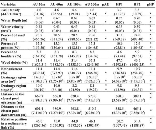
Table III. Average and variance (in parenthesis) of JAS density and selected environrnental variables for each size of analytical units (AU). HPI corresponds to the model developed with ail habitat patches, and NP2 corresponds to the model deveioped with habitat patches > 50 m. ANOVAs and Levene tests that are statisticaiiy significant
at the threshold of
p=O.O5
are marked with an * in the “pAU” colurnn for the testsbetween AU sizes, and in the “pHP” colurnn for the tests between AU sizes and HP models.
Variables AU 20m AU 60m AU 100m AU 200m pAU UPI 11P2 pHP
JAS Density 4.6 4.6 4.6 4.6 3.2 3.8 (JASIOOm2) (31.36) (22.56) (19.01) (15.44) * (11.76) (10.89) * 0.67 0.67 0.67 0.67 0.75 0.70 * Water Depth (m) (0.06) (0.04) (0.03) (0.03) * (0.05) (0.06) * Watervelocity 0.43 0.43 0.43 0.43 0.33 0.39 * (ms1) (0.05) (0.04) (0.04) (0.03) * (0.03) (0.03) * Percent ofsand 20.5 20.5 20.5 20.6 31.8 24.0 * (%) (465.26) (331.24) (288.66) (221.12) * (569.7$) (492.40) * Percent of 15.3 15.3 15.3 15.3 10.6 12.6 * pebbles(%) (155.50) (130.64) (118.81) (104.65) (95.84) (109.62) * Percent of 8.3 8.3 8.3 8.3 4.6 5.9 * boulders (%) (164.35) (151.78) (145.93) (134.56) (73.44) (97.61) * 31.4 31.4 31.4 31.3 47.5 40.5 * Wood debris(%) (1626.51) (1382.35) (1338.10) (1246.80) * (1592.81) (1409.25) * Embankment 11.4 11.4 11.4 11.4 9.9 10.7 (%) (439.74) (375.97) (340.77) (246.80) * (316.84) (254.40) * Drainage regÎon 3.6x10’ 1.1x10⁶ 1.9x10⁶ 3.9x10⁶ 1.9x10⁶ 3.9x10⁶ area (m2)l (2.50x10⁷) (2.25x10⁷) (3.$0x107) (7.62x107) * (4.0$x107) (8.35x10⁷) * Drainage region 10.0 10.0 8.2 8.1 * 9.8 9.3 * slope (°) (56.10) (56.10) (24.90) (19.27) * (43.96) (34.34) * Distance to the * 669.7 656.0 620.4 573.0 360.3 389.1 closest pool * (7.8$x105) (7.99x10⁵) (7.79x10⁵) (7.45x10⁵) (3.5$x105) (3.57x10⁵) upstream (m) Dïstance to the 601.4 580.9 563.8 510.2 358.5 465.1 * closest POOl (7.41x10⁵) (7.27x10⁵) (7.30x10⁵) (6.93x10⁵) (5.33x10⁵) (7.56x10⁵) downstream (w) Relative position * 45.0 45.0 44.9 46.1 60.2 51.4 * in a sedimentary (1267.36) (1270.92) (1272.35) (1302.49) (1007.43) (1188.87) link(%)
31
HABITAT QUALITY MODELS
The twenty-one datasets obtained following our sampling allowed us to develop twenty-one HQM. Bootstrap analyses indicated that the predictive power of HQM tended to increase as the size of AU increased from 20 (average R2adj. 0.3 1) to 200 rn (average R2adj= 0.61; figure 5). The 95% CI of the R2adj showed that the predictive power of HQM increased significantly as the size of AU increased from 20 (R2adj.
0.25-0.37) to 100 m (R2adj = 0.39-0.67). Although the R2adj ofrnodels developed using
AU of 200 rn (R2adj = 0.42-0.81) was higher than with AU of 100 rn, the gain in
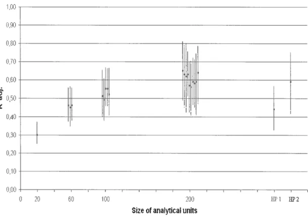
predictive power was not statistically significant. In addition, the range ofthe 95% CI of R2adj. associated with HQM tended to increase as the size of AU increased. The predictive power of HQM developed using alt habitat patches (HP 1) was sirnilar to that of models based on AU of 60 rn but lower than that of HQM developed using only habitat patches >50 rn (HP2; figure 5). R2adj of HQM developed using HP2 were similar to those based on AU of 200 rn.
32
E
O 20 60 100 200
Size of analytîcal unïts
Figure 5. Results ofthe bootstrap analysis. Bars represent 95% confidence intervals of
R2adj. for 1 000 iterations ofmodets developed using different sizes ofanalytical units
(AU). Squares represent original values ofR2adj..
•1,0O 080 R7 060 0,5’] n: 0-l0 0,30 Cii 010 0,00 BPIHP2
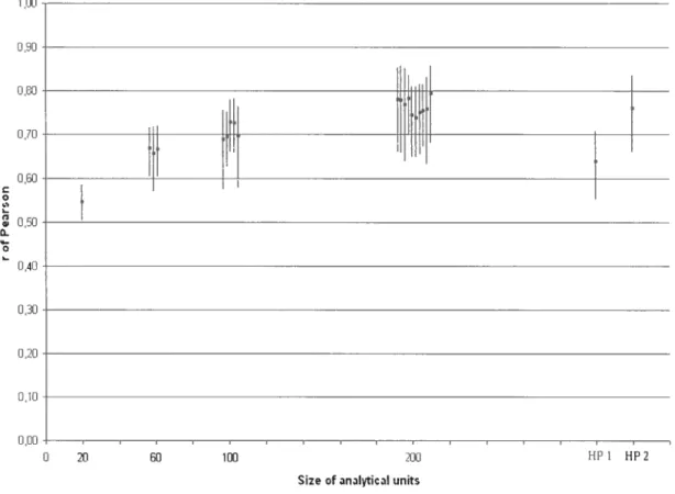
33 The cross-validation of the models we developed suggested that the upscaling of HQM was affected by the size of AU. Pearson correlation coefficients of relationships between JAS densities predicted using HQM based on AU of 20 m and observed values ranged from 0.5 1 to 0.58 (Figure 6). Corresponding values for HQM developed using AU of 200 m ranged from 0.64 to 0.86. This range extended from 0.56 to 0.71 for models developed using ail HP, and from 0.67 to 0.83 for those based on HP >50 rn. However, models developed using AU of 200 rn and HP >50 rn (HP2) were the only HQM for which the siopes and the intercepts of the relationship between predicted and observed JAS densities aiways had 95% CI that included, respectiveiy, the value of 1 (figure 7) and the value of O (Figure 8). Hence. ony eteven of the twenty-one HQM
developed explained significant proportions of the variation of JAS densities and could be upscaled to adequately predict JAS densities (Table IV).
34 0,90 0.00 o,io 0,60 C o w 00 Q o 0,40 0,30 0,20 o ,;o 0,00
Figure 6. Results of the cross-validation analysis. Bars represent 95% confidence intervals of r of Pearson of the relation between observed and predicted JAS density for 1 000 iterations of models developed using different sizes of analytical units (AU). Squares represent medians of r of Pearson.
t
t
0 20 60 00 200
Size of anaIticaIunits
35 ,1 1 2 D 0 o (I) O 3 D ,4 0,2 O
Figure 7. Resuits of the cross-validation analysis. Bars represent 95% confidence intervals of the siope of the relation between observed and predicted JAS density for 1 000 iterations of models developed using different sizes of analytical units (AU). Squares represent medians of siopes.
O 20 60 100 200 HP I HP 2
36 2,5 1,5 w w u -D .5 -1,5
figure 8. Resuits of the cross-validation analysis. Bars represent 95% confidence intervaïs of the intercept of the relation between observed and predicted JAS density for 1 000 iterations of models developed using different sizes of analytical units (AU). Squares represent medians ofintercepts.
llll
.E
4
D 20 BD 100 200 1 }2
Table IV. Habitat quality models that successfully predicted JAS density variations during the cross-validation exercise. Numbers in bold are partial R2adJ. Numbers in italic are the beta coefficients of each variable in the regression models. Size of analyfical units 200 in HP Dataset 1 2 3 1 5 6 7 8 9 10 2 Radj, 065 063 0.62 0.63 0.57 0.56 0.59 0.58 0.59 0.64 0.59 Depeudant variable JAS JAS JAS Ln JAS Ln JAS Lii JAS Lii JAS Ln JAS JAS JAS JAS 0.5$ 0.5$ 0.58 0.56 0.59 Boulders (,,) +0.208 +0.222 0.229 -0.230 -0.228 0.5$ 0.54 0.54 0.54 0.55 Lubou1ders) +0.315 +0.299 +0.305 +0.240 f0,3]] . 0.02 pla ofwood debris -] 390 . 0.03 0.03 0.02 0.03 tood debns ( /1) -0.006 -0005 -0.004 -0.005 0.05 0.05 0.03 0.05 0.05 p/a ofembankment a-1.832 --2.076 -1.630 2.062 ‘].84 Lu embankment (%) 0.01 -0.6b 0 0.03 Sandy shore -0.013 . 0.02 Lu dist. to tise closest pool downstream (in) 0 039 . . . 0.02 Distance to the closest spawning site upstream (km) -6 3y ]0’ . . . . . . 0.54 Ln relative position in a seduuentary hnk (%) -] 81 Intercept —2.965 -h-1.781 ±1847 ÷1.384 —1.219 +1.202 +1.542 —1.194 —1.896 —1.673 +9.688
‘D
3$ The percent contribution of boulders to the riverbed explained the rnajority the variance of parr density in ail models developed using AU of 200 m (0.54 < partial
R2adj < 0.59). Wood debris, another local variable, was selected in haif of the HQM
developed using AU of 200 rn (0.02 < partial R2adj < 0.03). Embankment, a laterai
variable, was included in half of the 200 m models. Embankrnent was aiways as the second most important variable in the model (0.03 < partial R2adj < 0.05). The
percentage of sandy shore (lateral variable) also contributed to explain a fraction of the variations of]AS density (partial R2adj =0.03). f inaily, the distance to the nearest pool
downstream (R2adj = 0.02), and the distance to the nearest spawning site upstream
(R2adj = 0.02) were the two longitudinal variables that explained a significant fraction of
JAS density in models developed using AU of 200 m.
Contrary to the models developed with AU of 200 m, the HP2 mode! exclusively included spatial context variables. In this mode!, the variable that had the rnost signfficant effect on JAS density Qartial R2adj. =0.54) was the relative position ofa AU
in a sedimentary link. The other spatial context variable included in this model was the presence or the absence ofembankment (partial R2adj.= 0.05).
DISCUSSION
flJFLUENCE 0F THE SIZE 0F ANALYTICAL UNITS
The results of our analyses are consistent with the expectations associated with the modifiable areal unit problem (MAUP; Jelinski and Wu 1996), also referred to as the
39
scale dependence problem (Wiens 1989; FoIt et al. 1998). The size of AU had a significant effect on attributes of HQM. For instance, the average R2adj of HQM
increased as the AU size increased from 20 ni to 200 ni. Two hypotheses may be used to
explain effects of AU size on HQM attributes. First, the nature of the independent variables used during this study to develop HQM may hamper the ability of these models to explain JAS density variations when AU are small (e.g. 20-60 m) and facilitate the finding of more powerful models when AU are large (200 m, HP2). In the present study, only physical variables were employed to model JAS density variations because they are generally easier to estimate than biological variables such as prey availability, competition, and predation. Yet, it has been suggested that, as the size of AU decreases, the magnitude of the effect of biological variables on the distribution of the biota increases while that ofphysical variables decreases (Legendre 1993; Jackson at al. 2001; Brind’Amour et al. 2005). Our findings that the development of powerful HQM based on small AU is difficult without biological variables and that the predictive power ofHQM based on physical variables increases as AU size increases are consistent with this suggestion. Second, it may be more difficult to develop strong predictive models with srnall AU (e.g. 20-60 ni) because the error associated with JAS density in
small AU may be larger than that in large AU (200 m; HP2, habitat patches > 50 m). In
our study, JAS density was estimated only once in any given AU. Bouchard et al. (unpublished data) estimated JAS density on ten occasions in four 200 m reaches ofthe
SIVIR tising a sampling method identical to that used in the present study. They found that the coefficient of variation of JAS density decreased from 120% to 60% as AU size increased from 10 to 200 m. They attributed this situation to the possibility that, although JAS are generally described as territorial fish, they may move tens to hundreds
40
of meters over few days (Arrnstrong et al. 1997; Metcalfe et aI. 1997; Økland et al. 2004; Booker et al. 2004) Hence, this interpretation and our findings are consistent with the suggestion of Bellehumeur and Legendre (1997) that the use of larger AU may diminish the noise found in spatial data and inctease the ability to develop statistically significant models.
The performance of HQM based on relatively large AU was also expressed during the upscaling ofthe models we developed. HQM based onAU of 200 m and HP2 model taken from one third of the segments were the only models that could be effectively upscaled to the other two thirds of the segments. We wotild argue that two elements contribute to the similar performance of HQM developed using AU of 200 m and HP > 50 m. f irst, the size of habitat patches in the HP2 data set averaged 193 m
(range from 60 m to 1 140 m) which confers to HP larger than 50 m the same kind of statistical advantage (lower coefficients of variation) as AU of 200 m. Second, the fact that the size of 200 m AU is similar to that of the average HP confers to AU of 200 m the same ecological advantages as HP. HP, which are spatially continuous units possessing relatively homogeneous environmental characteristics, may represent more ecologically meaningftul AU than AU of an arbitrary size defined iliespective of any environmental variable (Brind’Amour and Boisclair 2006). In this context, one may expect that HP >50 m would allow the developmeiit of HQM more powerfiul than AU of 200 m. However, we found that the R2adj. of HP2 model (0.59) was slightly lower than that of HQM based on AU of 200 m (average = 0.6 1). Whether this is caused by the presence of smaller patches (50 to 200 rn) in HP2 caimot be evaluated because of an insufficient number ofpatches >200 m in this data set (17; figure 3).
41
INFLUENCE 0f TUE SPATIAL CONTEXT 0F ANALYTICAL UNITS
The HQM we developed potentially included the effect of local variables (environmental conditions observed within AU) and spatial context variables (environmental conditions observed outside AU). However, the moUds that had the best predictive abilities (AU of 200 m and HP >50 ni) differed in their structure and, in particular, in the relative importance ofthese types of variables for HQM. Seven ofthe ten HQM based on AU of 200 m included the combined effects of local (0.02 <partial R2adj < 0.59) and spatial context variables (0.02 <partial R2adj < 0.05). Among the
local variables, the percentage of boulders contributed most to explain the variations in JAS density (0.54 < partial R2adj < 0.59). The effect of this variable may be related to
the expectation that the size of JAS teiiitory should decrease as the contribution of boulders to a riverbed increases due to a visual isolation between them (Kalleberg 1958; Dolinsek 2004). Wood debris is a local variable included in half of the 200 un models. Wood debris tended to have a negative effect on JAS density. However, Bouchard et al. (unpublished data) found a positive relationship between wood debris and JAS density in the SMR. We explain this inconsistency by the study extend difference existing between their study and ours. Their data have been collected in sites located ail along the SMR, where wood debris are found in ail habitat types. In contrast, our data were concentrated in a specific 14.7 km section where wood debris were particularly associated with the meanders sections. Indeed, in our study, there is a positive relationship between the percentage of sand and the presence of wood debris (with AU of 200 rn; r of Pearson= 0.30, p < 0.05). Furtherrnore, in the 200 m datasets, only 20 %
of the AU contain wood debris and boulders (> 15
%).
It is thus possible that, in our study, the effect of wood debris on JAS density was masked by the effect of substrate.42
Yet, wood debris were particularly found in habitats where JAS were already less abundant.
Arnong the spatial context variables, the variables that described attributes of the shore (lateral variables) explained, on average, 3 % (negative effect of the presence of sandy beaches) to 5 % (positive effect of the presence ofernbankrnents) of JAS density variations. Both variables confirrned the positive effect of the presence of large substrate on JAS density. Longitudinal variables that expressed the cffect of the distance between AU and specific features of the river explained 2 % (distance of the nearest pool downstream, and distance to the nearest spawning site upstrearn) of JAS density variations. Gries and Juanes (199$) docurnented that pools represent daytirne sheltering habitats against high water temperatures, highly turbulent flows, intra-specific competition, and predation. Ouï analyses, suggest that JAS also tend to be associated with pools at night. This observation, together with the expectation that intra-specific competition and predation should be lower at night (Poff and Huryn 1998), indicate that physical conditions such as cooler water temperatures and less turbulent flows may be the primary conditions attracting JAS to pools and that, if there is any structure to this behaviour, parr tend to move upstream of a pool at night. However, further studies may be needed to conflrm this behaviour. JAS density was negatively related to another longitudinal variable; the distance to the closest spawning site, this tirne, upstream of AU. This relationship may be related to sedentary behaviour that favour the use of nursery habitats close to the spawning site and, when movernents do occur, to a passive behaviour that transport JAS, particularly during their first year of life, towards the closest nursery areas downstream of spawning sites (Beail et al. 1994).
43
In contrast with moUds based on AU of 200 ni, the onÏy HQM based on HP >50 ni cornprised exclusively spatial context variables. The position of AU within a
sedirnentary link (longitudinal variable) explained 54 % of the variation of JAS density while the presence ofernbankment (lateral variable) explained 5 % ofthis variation. Our analyses therefore stiggest that JAS density tended to decrease as the distance from AU to the upstream luit ofa sedimentary link increased. Hence, the identity ofthe variables that cxplained the largest fraction of JAS density differed between moUds developed using AU of 200 ni (percent contribution of boulders) and HP >50 ni (position within a
link). However, the percent contribution of boulders to the riverbed is related to the position of habitat patches within a sedirnentary link (r ofPearson = 0.6$ for HP2). The elimination of the variable ‘position within a sedimentary link’ fiom the analysis perforrned to develop HQM based on HP2 resulted in the finding of a new model in which the percent contribution of boulders to the riverbed (partial R2adj 0.45) and the presence of embankrnent (partial R2adj.= 0.07) explained 52% of the variations of JAS density. These analyses, together with the knowledge that the upstream limits of sedimentary links are characterized by the dominance of boulders (Rice et al. 2001) suggest that models developed for HP2 using either local or spatial context variables maybasically emphasize the same biological relationship between JAS and boulders.
CONCLUSION
Taken together, our study is consistent with the expectation that changing the size of AU may affect the structure and the predictive ability of HQM. Our analyses