HAL Id: hal-01169750
https://hal-mines-albi.archives-ouvertes.fr/hal-01169750
Submitted on 30 Jun 2015
HAL is a multi-disciplinary open access
archive for the deposit and dissemination of
sci-entific research documents, whether they are
pub-lished or not. The documents may come from
teaching and research institutions in France or
abroad, or from public or private research centers.
L’archive ouverte pluridisciplinaire HAL, est
destinée au dépôt et à la diffusion de documents
scientifiques de niveau recherche, publiés ou non,
émanant des établissements d’enseignement et de
recherche français ou étrangers, des laboratoires
publics ou privés.
Shape Measurement Using a New Multi-step
Stereo-DIC Algorithm That Preserves Sharp Edges
J. Harvent, Benjamin Coudrin, L. Brèthes, Jean-José Orteu, Michel Devy
To cite this version:
J. Harvent, Benjamin Coudrin, L. Brèthes, Jean-José Orteu, Michel Devy. Shape Measurement Using a
New Multi-step Stereo-DIC Algorithm That Preserves Sharp Edges. Experimental Mechanics, Society
for Experimental Mechanics, 2015, 55 (1), pp.167-176. �10.1007/s11340-014-9905-z�. �hal-01169750�
(will be inserted by the editor)
Shape Measurement Using a New Multi-Step Stereo-DIC
1
Algorithm That Preserves Sharp Edges
2
Jacques Harvent · Benjamin Coudrin · Ludovic 3
Br`ethes · Jean-Jos´e Orteu ·
4
Michel Devy 5
Received: date / Accepted: date
6
Abstract Digital Image Correlation is widely used for shape, motion and deforma-7
tion measurements. Basically, the main steps of 3D-DIC for shape measurement 8
applications are: off-line camera calibration, image matching and triangulation. 9
The matching of each pixel of an image to a pixel in another image uses a so-10
called subset (correlation window). Subset size selection is a tricky issue and is 11
a trade-off between a good spatial resolution, achieved with small subsets that 12
preserve image details, and a low displacement uncertainty achieved with large 13
subsets that can smooth image details. 14
In this paper, we present a new multi-step DIC algorithm specially designed 15
for measuring the 3D shape of objects with sharp edges. With this new algorithm 16
J. Harvent
NOOMEO, 425 rue Jean Rostand, F-31670 Lab`ege, France E-mail: jacques.harvent@gmail.com B. Coudrin
CNRS ; LAAS ; 7 avenue du colonel Roche, F-31400 Toulouse, France
Universit´e de Toulouse ; LAAS ; F-31400 Toulouse, France E-mail: bcoudrin@laas.fr L. Br`ethes
NOOMEO, 425 rue Jean Rostand, F-31670 Lab`ege, France E-mail: ludovic.brethes@noomeo.eu J.-J. Orteu
Universit´e de Toulouse ; Mines Albi ; ICA (Institut Cl´ement Ader) ; Campus Jarlard, F-81013 Albi, France E-mail: jean-jose.orteu@mines-albi.fr
M. Devy
CNRS ; LAAS ; 7 avenue du colonel Roche, F-31400 Toulouse, France
an accurate 3D reconstruction of the whole object, including sharp edges that are 17
preserved, can be achieved. 18
Keywords Shape Measurement·Stereovision·Digital Image Correlation (DIC)·
19
Edge Preservation·Accurate 3D reconstruction. 20
1 Introduction 21
The problem of improving the accuracy of the 3D reconstruction of a complex 22
object is addressed by using a DIC-based shape measurement technique. The DIC 23
technique requires choosing a correlation criterion, the size of the correlation win-24
dow (also called subset) and the window transformation model (subset shape func-25
tion). The choice of the subset size is a tricky issue [1–4] and is a trade-off between 26
a good spatial resolution, achieved with small subsets that preserve image details, 27
and a low displacement uncertainty achieved with large subsets that can smooth 28
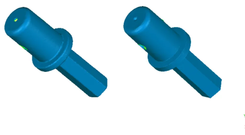
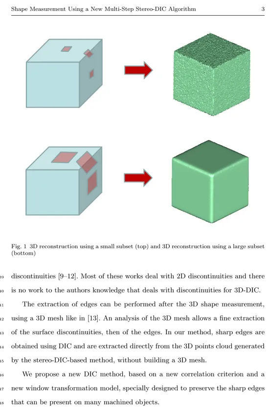
image details (see figure 1 and table 1). 29
subset size displacement uncertainty shape details
small high preserved
large low smoothed
Table 1 Trade-off between displacement uncertainty and shape details preservation
In order to increase the accuracy of the shape reconstruction, several authors 30
have proposed to use a multi-view stereo method that exploits a large number of 31
images [5–8] and that allows using a small subset size. 32
In this paper, we address the problem of providing an accurate 3D reconstruc-33
tion of an object by using the classical two-views 3D-DIC technique. 34
In the classical DIC-based matching technique, discontinuities (e.g. cracks 35
in 2D-DIC-based displacement/strain measurements, sharp edges in stereo-DIC-36
based shape measurements) are difficult to handle and several authors have pro-37
posed new DIC formulations specially designed for DIC matching in presence of 38
Fig. 1 3D reconstruction using a small subset (top) and 3D reconstruction using a large subset (bottom)
discontinuities [9–12]. Most of these works deal with 2D discontinuities and there 39
is no work to the authors knowledge that deals with discontinuities for 3D-DIC. 40
The extraction of edges can be performed after the 3D shape measurement, 41
using a 3D mesh like in [13]. An analysis of the 3D mesh allows a fine extraction 42
of the surface discontinuities, then of the edges. In our method, sharp edges are 43
obtained using DIC and are extracted directly from the 3D points cloud generated 44
by the stereo-DIC-based method, without building a 3D mesh. 45
We propose a new DIC method, based on a new correlation criterion and a 46
new window transformation model, specially designed to preserve the sharp edges 47
that can be present on many machined objects. 48
2 Overview 49
The presented method is an extension to the standard stereo-vision 3D recon-50
struction. It aims to refine the reconstruction accuracy for points near sharp 51
edges. These points are generally badly estimated due to an over-smoothing effect. 52
Standard stereo-vision uses the approximation that the observed surface is locally 53
continuous and almost planar. This assumption becomes false near sharp edges 54
causing a false estimation of the surface. Due to the planar approximation, stan-55
dard stereo-vision tends to measure edges as curves. To achieve the sharp edges 56
preservation, our proposed method performs an iterative refinement of the areas 57
where the planar approximation fails. It starts from an initial 3D reconstruction 58
of an object. 59
The initial 3D reconstruction is obtained using a standard stereo-vision method 60
and is briefly presented in section 4. It provides a 3D point cloud representation of 61
the surface, and equally computes normals and confidence values of the measured 62
points. 63
From this initial reconstruction, our edge-optimized method refines iteratively 64
the position of the edges. Our algorithm is composed of three steps. 65
Firstly, it detects regions with high curvature. These regions are considered candi-66
dates to the edge refinement. This allows us to reduce the number of points which 67
need to be processed. It is presented in section 5. 68
Secondly, the algorithm computes a first estimate of the possible location of the 69
edges for each area (section 6). 70
Finally, every considered point is estimated using our new ”bi-plane” model. This 71
model is based on the two planes which compose an edge, and is refined minimizing 72
a correlation criterion. It is presented in section 7. 73
The proposed strategy to improve the accuracy near sharp edges is itself based 74
on a two-planes assumption, i.e. the neighborhood of every point on the object 75
surface can be approximated by two planes. In some situations (chamfers perceived 76
from a far viewpoint), this assumption can be violated. An additional step is 77
necessary to validate the results. The residual error from the standard stereo-vision 78
method and the residual error from our new edge-optimized method are compared. 79
The reconstruction which provides lower error is chosen. This ensures that high 80
curvature areas not representing actual sharp edges would not be ”sharpened” by 81
error. 82
3 Problem formulation and notation 83
We consider a stereo-vision system with two digital cameras rigidly attached. We 84
associate to each camera an euclidean coordinate frame. RespectivelyC0 andC1
85
for the principal camera and the secondary one: 3D points are reconstructed in 86
the reference frame of the principal camera. Every camera is calibrated using the 87
method from [14], modified to allow automatic initialization; the rigid transfor-88
mation between the reference frames of the two cameras is also estimated using 89
the standard stereo calibration toolbox. Images are considered distortion free – 90
i.e. the images are provided by a perfect distortion free system or the images have 91
been corrected from their distortion using the calibration parameters. Moreover, 92
images and transformations are considered in the epipolarly rectified space. This 93
transformation between the cameras is noted [I3×3|tC1C0]∈ SE(3), whereI3×3is a 94
3×3 identity matrix andtC1C0is the translation between the origins of the camera 95
frames, with only the baseline along theX axis. 96
The stereo-imaging process can then be represented using a linear model re-97
lating a 3D point in the world (reference) coordinate frame mW = (X, Y, Z,1)T
98
to two image pointsmI0 = (sx0, sy, s)
T and
mI1= (sx1, sy, s)
T the projections of
99
mW in, respectively, the image coordinate framesI0, related to the cameraC0, and
100
I1, related to the cameraC1. Due to the epipolar rectification, images of the same
101
3D points lie on the same image line and have then the sameycoordinate [15]. 102
The imaging process can be formulated as follow.
mI0 =K0[RC0W|tC0W]mW (1)
mI1 =K1[I3×3|tC1C0] [RC0W|tC0W]mW (2)
whereK0andK1are the calibration matrices of, respectively, camerasC0and
103
C1, formed from the cameras independent intrinsic parameters, and [RC0W|tC0W]∈ 104
SE(3) is the transformation between the world frameWand the principal camera 105
frameC0. This transformation is called the pose of the system.
106
4 Initial reconstruction 107
Standard stereo-vision reconstruction is the process of finding the 3D point coor-108
dinatesmW from its image pointsmI0 andmI1. 109
A common stereo-reconstruction approach is to try to match pixels in the 110
pair of images using the luminance information of the images. This is achieved by 111
determining the pointmI1matching the pointmI0. This is done by observing and 112
matching luminance information in both images,I0andI1. Luminance functions
113
are notedI0(p) andI1(p), respectively for imagesI0andI1. To avoid ambiguities,
114
the matching point is found by comparing local appearance around the pixelmI0. 115
Surface can be approximated locally by tangent planes to observed points. The 116
matching process is the similarity measurement of the projections of an area of this 117
approximated plane in the images. The transformation relating the projections in 118
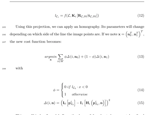
each image is an homography (figure 2). 119
From [8] we have the following homography formulation: 120
π
WC
0C
1H
Fig. 2 An homography is a projective transformation relating the projections of a plane in two images H=K1[I3×3|tC1C0]SK −1 0 (3) S= 2 6 6 6 6 6 6 6 6 4 −1 0 0 0 −1 0 0 0 −1 nx ny nz 3 7 7 7 7 7 7 7 7 5 (4)
where (nx, ny, nz)T is the normal of the tangent plane to the surface atmW.
121
The structure of the scene, from two images acquired at the same time, is 122
obtained by minimizing dissimilarities between the luminance function I0(p) in
123
the region W of imageI0 and the luminance function I1(p) in the transformed
124
regionH(W) of image I1. If we notex= (nx, ny, nz), we try to find
125 argmin x X i∈W “ I0 h piI0 i − I1 h Hi “ piI0, x ”i”2 (5)
Equation (5) introduces the minimization criterion used to find, for a given 126
pointmI0, the matched pointmI1, using only the parameters of the tangent plane 127
defined by the correlation of two pixel regions in two stereo images. This problem 128
can be solved using standard non-linear least-squares methods. 129
This approach is valid and has proved to work well on nearly planar surfaces. 130
The assumption that the observed regionW is a plane tangent to surface atmW
131
introduces an approximation resulting in a surface smoothing (figure 3). 132
Fig. 3 The plane model does not fit the surface along the edges
The reconstruction process on very non-planar surfaces is a trade-off between 133
accuracy and stability by tuning the size of the regionW. 134
Particularly, when the region W contains sharp edges, the tangent plane-135
induced homography is not a valid model. It tends to reduce the discontinuity 136
of the surface. Our method proposes to correct the result of the process we have 137
described by detecting sharp edges in the model and re-correlating the erroneous 138
points using a ”bi-plane” model. 139
5 Edge detection 140
The aim of our proposed method is to refine the initial reconstruction we have 141
presented to allow reconstruction of sharp edges. Only the points near sharp edges 142
have to be refined. To avoid processing unnecessary points, we add an edge detec-143
tion step. 144
Since the method we have described tends to smooth discontinuities due to the 145
approximation of the local surface, edges are reconstructed as short arc curves. 146
For each 3D point p0, with its normal n0, let us consider the neighborhood W
147
consisting of nearest points pi ∈ W aroundp0. Each pointpi is associated with
148
its normal ni. We compute the mean normal ¯n, the mean µ and the standard
149
deviationσof the dot products to this mean normal inW. 150 ¯ n= 1 kP i∈W(p0)nik X i∈W(p0) ni (6) µ= 1 card(W(p0)) ¯ n · X i∈W(p0) ni (7) σ= v u u t 1 card(W(p0)) X i∈W(p0) (n · n¯ i− µ)2 (8)
Points on short arc curves are identified from high deviation regions to ensure 151
that we select regions with high curvature. The standard deviation σ of the dot 152
products represents the variability of the normal distribution in W and is then 153
used as the deviation measurement. 154
The detection process consists in thresholding the standard deviation σ. The 155
criterion is used to build a selection functionΠ(p). 156 Π(p0) = 8 > < > : 1if σ(p0)> α 0 otherwise (9)
where α is the threshold, allowing to be more or less selective on the edge 157
detection. A higher threshold will reject more points, increasing the probability of 158
non-detection. A lower threshold will result in a less selective behavior, increasing 159
the probability to select non-edges points. 160
The edge selection process allows us to save time by processing less non-edge 161
points. The results of our method is not likely to improve points that do not lie 162
on edges. We discuss in section 7.2 this matter and how we deal with wrongly 163
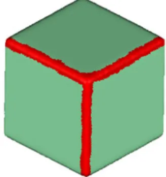
selected points. 164
Fig. 4 Selection (red) of the edges of the cube
6 Initial edge estimation 165
An initial estimate of the edge model is computed for each selected point, and this 166
estimate is refined later (as described in section 7). The edge model consists of two 167
mean normals each of which describes one face of the edge. In order to compute 168
these two normals, we consider a region around the edge and then we classify 169
the points and their normal in two groups using a modified k-means clustering 170
algorithm. In section 5 the standard deviationσof the dot products to the mean 171
normal was computed for each point. This value is introduced in the clustering 172
process, in order to filter points with a large σ. A plane is then fitted to each 173
cluster of points. The result provides the two mean normals. 174
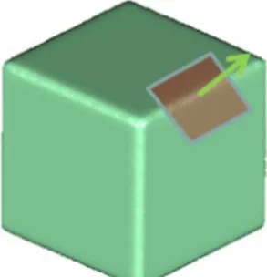
7 Edge preservation 175
7.1 Edge matching 176
In order to refine points along edges, we introduce a new surface model. This 177
model is represented by two planes which intersect as a 3D lineL(figure 5). 178
Fig. 5 The ”bi-plane” model is represented by two planes defined by their normals (green)
The intersection can be expressed as Pl¨ucker axial coordinates: 179
L= [L23:L31:L12:L01:L02:L03] (10)
with Lthe Pl¨ucker matrix. 180
Given two planesπ0= (n0,1)T andπ1= (n1,1)T, withn0andn1 the normals
181
of the planes, Pl¨ucker axial coordinates of their intersection are defined as: 182
L= [n1− n0:n0× n1]T (11)
where ×is the cross product. 183
The projection of a 3D lineLon a 2D linelinCi coordinate frame is written:
lCi=f(L, Ki[RCiW|tCiW]) (12)
Using this projection, we can apply an homography. Its parameters will change 185
depending on which side of the line the image points are. If we notex=“nT0, nT1
”T
, 186
the new cost function becomes: 187 argmin x X i∈W φ∆(i, n0) + (1− φ)∆(i, n1) (13) with 188 φ= 8 > < > : 0if lC0· x <0 1 otherwise (14) ∆(i, n) =“I0 h piI0i− I1 h Hi “ piI0, n”i”2 (15)
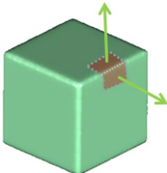
This new ”bi-plane” model allows the shape of the edge to be accurately refined 189
as seen in Figure 6. 190
Fig. 6 3D reconstruction of the cube using the edge-optimized method (to be compared with figure 1)
7.2 Edge consistency 191
The proposed edge model produces good results along sharp edges made of two 192
faces. However, problems may occur when the edge model is used on surfaces with 193
chamfers, spikes, small radii edges of fillets. 194
Both chamfers and spikes are composed of more than two planes. Small radii 195
are not a surface discontinuity. In any case, our edge model cannot fit the surface 196
perfectly. In the case of important noise on the surface, the algorithm may be 197
biased and result in incorrect bi-plane fitting. 198
To prevent our method to include sharp edges in the model where they must 199
not be or to accept inconsistent results we have added a verification step. 200
In order to discard wrong results produced by the edge optimization, we com-201
pare results obtained by the standard criterion to results obtained by the edge 202
optimization and choose the best one. This works as both methods minimize a 203
sum of squared differences on pixel intensity. 204
In addition we can set a threshold on the angle between the two-plane fitted by 205
our algorithm to reject flat angles, that are mostly inconsistencies due to surface 206
noise. 207
8 Results and discussion 208
The results presented in this section have been processed from images of a home-209
made stereo-vision system. It is composed of two 1024×768 CCD cameras with 210
8 mm lenses and a pattern projector. The stereoscopic baseline is 140 mm long 211
and the cameras are oriented with a 15◦ angle. The working distance is about 212
400mmand the pixel size is about 0.23mm. During the image correlation process, 213
11×11 pixel correlation windows are used, leading to a spatial resolution of about 214
2.5×2.5 mm2. The whole setup has been described and evaluated by Coudrin 215
et al. [7]. The cameras and the projector are synchronized. We use a pattern 216
projection to provide a dense 3D information from the pair of cameras, regardless 217
of the texture on the object surface. When the system is triggered, the pattern is 218
projected on the scene. Then the two cameras acquire images simultaneously. The 219
pair of images is used in a reconstruction algorithm, providing a 3D point cloud by 220
a stereo-vision surface reconstruction method. Points are expressed with respect 221
to the frameC0 of the principal camera.
222
Figure 7 presents two 3D reconstructions of a mechanical part. The part con-223
tains both sharp and curved edges. On the left, one can see the result of the initial 224
reconstruction. Sharp edges are rounded. On the right, one can note that the sharp 225
edges have been corrected and are sharper. Curved edges have not been modified. 226
Fig. 7 Result of standard 3D reconstruction (left) and edge-optimized 3D reconstruction (right)
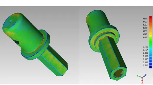
To illustrate the improvement of the new method, the deviation between the 227
two results has been computed using Geomagic Qualify software (figure 8). The 228
color map describes the signed euclidean distance between the two shapes and lies 229
within the range [−0.5mm,+0.5mm]. The largest errors can be observed along the 230
edges. It shows that points on edges have moved up to 0.5mm from their initial 231
position. 232
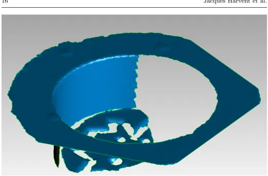
Figure 9 shows a cylindrical gauge block. It is composed of a section of a 233
cylinder with flat surfaces on the top and the bottom and perfectly circular surface 234
Fig. 8 Comparison between standard 3D reconstruction and edge-optimized 3D reconstruction. The color map represents the euclidean deviation between the two shapes
on the inside. The CAD model of this part is known and accurate up to 1µm. 235
Figure 9 shows the initial reconstruction of the cylinder. Figure 10 presents the 236
qualitative result of edge optimization. The edge at the intersection of the inner 237
cylinder and the top surface has been sharpened. The other edges have not been 238
altered since they are not actual sharp edges. 239
Since the CAD model is known for this part, we have evaluated the accuracy of 240
our method by comparing the 3D reconstruction results to the theoretical surface. 241
We have used the Geomagic QualifyTM software to align and compare our result 242
to the CAD model ground truth. The software gives a comparison by projecting 243
orthogonally each point of our 3D reconstruction to the surfaces of the CAD model. 244
The result of the comparison is a distance map. Small projection distances are 245
displayed in green, and tend to dark red or dark blue when the distance increases. 246
Figure 11 shows the distance map of the initial 3D reconstruction to the CAD 247
model. The error increases strongly on the edge. Indeed, the initial reconstruction 248
over-smoothes this sharp edge. Consequently, the points have been estimated far 249
behind the actual surface. After the edge optimization process, Figure 12 shows 250
Fig. 9 Initial 3D reconstruction of a cylinder
Fig. 10 Edge-optimized 3D reconstruction of the cylinder
the improved result. The edge has been accurately reconstructed and all the points 251
on the edge are in the acceptable green range. 252
As a side effect of our method, one can note that the top surface contains a 253
certain amount of error in figure 11 that is minimized in figure 12. This is due to the 254
Fig. 11 Distance map of the initial 3D reconstruction to the CAD model
Fig. 12 Distance map of the edge-optimized 3D reconstruction to the CAD model
alignment step of the Geomagic Qualify software. Since the initial reconstruction 255
contains more error, it is harder to align with the actual surface. With the edge 256
improvement, the 3D reconstruction is more accurate and can be more easily 257
aligned to the CAD model. 258
It should be noted that we have shown in [8] that the standard stereo-DIC 259
approach does not perform well with a small window size (3×3 or 5×5 pixel 260
windows). Indeed, reducing the window size increases ambiguities in correlation 261
and causes drifts in the stereo matching process, causing noise and holes in the 3D 262
reconstruction. On the contrary, with a 11×11 pixel window, the noise is reduced 263
and no holes appear, but the window becomes too large compared to the size of 264
some small details, causing a smoothing effect (see Figure 10 in [8]). With the new 265
multi-step stereo-DIC method proposed in this paper, a 11×11 pixel window can 266
be used while reducing the smoothing effect. 267
8.1 Accuracy comparison 268
To give an absolute reference of the results provided by our method, we used a 269
gauge block with a known geometry. 270
This part has been designed for measurement device calibration. It has been 271
accurately manufactured and has an accurately known geometry. It is composed 272
of several simple geometrical primitives (figure 13). 273
The ground truth CAD model (figure 14) is available and used to evaluate the 274
reconstruction error. 275
We compare our edge-optimized method to the standard pairwise stereovision 276
approach. As we have seen previously, this approach tends to smooth details and 277
edges. The gauge block is made of a large plane and geometrical primitives inter-278
secting the plane, creating sharp edges. We also provide results obtained with the 279
multi-view stereovision (MVS) method presented in [8]. 280
Models resulting from the three methods (pairwise stereovision, edge sharpen-281
ing in pairwise stereovision and our multi-view stereovision method) are registered 282
on the CAD model of the gauge block. Points are projected orthogonally on the 283
surfaces of the theoretical model and projection distance is measured for each 284
point. This distance is considered as the reconstruction error of the point. Figure 285
15 represents these errors using a color map. Green areas are measured inside 286
Fig. 13 The gauge block composed from simple geometrical primitives. It contains several sharp edges
the tolerance range [−25µm,+25µm]. Points with a larger positive error are rep-287
resented on a scale from yellow to red. Points with a larger negative error are 288
represented on a scale from light to deep blue. 289
As expected, the error map of the pairwise stereovision method shows a large 290
error near edges of the model. Due to the smoothing effect of the surface ap-291
proximation in the reconstruction process, edges are rounded. The error on the 292
dominant plane is essentially contained in the tolerance range. The edge-optimized 293
Fig. 14 The CAD model of the object is used as ground truth
Pairwise Edge MVS
stereo optimization optimization
Max error (mm) 0.553 0.478 0.452
Min error (mm) −0.606 −0.286 −0.446
Pos. mean (mm) 0.036 0.037 0.023
Neg. mean (mm) −0.032 −0.031 −0.020
Std. dev. (mm) 0.066 0.049 0.033
Table 2 Reconstruction error to the ground truth of the gauge block. Max/Min error : maximal positive and negative errors. Pos./Neg. mean : means of, respectively, positive and negatives errors. Std. dev : standard deviation on the error set
method performs a lot better along the edges. Maximal errors are now mainly lo-294
cated near complex edges – intersection of more than two surfaces – and along 295
the chamfer of the central drilling. However, a small error on the edges remains. 296
With our method, error is still mainly located near edges, but the model is more 297
homogeneously inside the tolerance. The chamfers in the central drilling are now 298
more finely reconstructed. It is to be noted that the dominant plane is also more 299
finely reconstructed. A significantly larger part of the object is considered inside 300
the tolerance comparing to the other methods. 301
Table 2 summarizes the results for this experiment. The results are presented 302
showing maximal and minimal errors. The mean error should be 0 mm, since the 303
models are registered minimizing the distance between point clouds and the surface 304
(a) Pairwise stereo
(b) Edge-optimized method
(c) MVS method
Fig. 15 Comparison of reconstruction error using pairwise stereovision, pairwise stereovision with our edge detection and correction method, and our multiview stereovision method
of the CAD model. It is then more meaningful to present average errors in positive 305
and negative parts. The standard deviation on the error set is also presented. 306
As it was pointed in figure 15, our edge-optimized algorithm and our MVS 307
method present better results and a higher accuracy in terms of deviation to 308
the theoretical surface. The MVS method offers the best results, with the lowest 309
deviation, but requires more images to be efficient. 310
8.2 Discussion 311
We have introduced a new bi-plane model and a new correlation criterion in order 312
to achieve a high accuracy 3D reconstruction along sharp edges. Standard window-313
based methods suffer from the tradeoff between higher accuracy obtained with 314
large subsets and more details obtained with small subsets. Our model permits 315
to use larger subsets with the advantage of having both more details (reduced 316
smoothing effect) and higher accuracy along the edges. 317
The main advantage of our method is that it performs well with a single stereo 318
pair of images. Most of the state of the art methods which produce high accuracy 319
3D reconstruction rely on multiple views. Even if most of these methods perform 320
better than our new bi-plane model, our method allows to improve the reconstruc-321
tion along sharp edges when a multiple view configuration is not possible. This 322
may be the case for those industrial applications where the number of cameras is 323
limited or when the shape to be measured is not easily accessible. 324
The actual limitation of our method is that it only handles one kind of discon-325
tinuity: a bi-plane edge. With this model, more complex edges are not correctly 326
modeled and are generally smoothed. Nevertheless, the general methodology de-327
scribed in this paper could be extended to handle more complex edge models 328
(and associated correlation criterion) and a model switching mechanism could be 329
implemented. By using the verification step described in section ”7.2 Edge consis-330
tency” the model leading to the minimal correlation score could be kept locally. 331
The choice of the best model could be even made easier in situations where the 332
CAD model of the object to be reconstructed in 3D is available. 333
9 Conclusions and Future Work 334
We have developed a new multi-step stereo-DIC algorithm, based on a new cor-335
relation criterion and a new window transformation model, specially designed for 336
measuring the 3D shape of machined objects with sharp edges. 337
With a standard stereo-DIC-based shape measurement technique, sharp edges 338
are generally smoothed. This effect can be minimized by choosing small size subsets 339
but this increases the stereo matching uncertainty. 340
With our new method, reducing the subset size to avoid smoothing sharp edges 341
is not necessary. 342
Results on real machined objects show that, with our new method, an accurate 343
3D reconstruction of the whole object, including the sharp edges that are preserved, 344
can be achieved. 345
Many methods for 3D reconstruction are iterative and multi-resolution, im-346
proving an initial low-resolution model up to a representation with the required 347
resolution and accuracy. Future work will be devoted to such a method, including 348
using a prior knowledge provided by the object CAD model when available, in 349
order to make simpler and more accurate the modeling process. 350
We also compared our method to a MVS method. Although the accuracy of 351
MVS methods is better than our edge-optimized method, the latter requires only 352
one pair of images and is able to produce honorable results. MVS methods require 353
several images. It is legitimate to ask if combining both methods (MVS and edge 354
optimization) and working with several images would improve the results. 355
DIC is widely used for shape and strain measurement. This work focused on 356
shape measurement and we did not explore the eventual contribution of the edge-357
optimized method to strain measurement. This will be part of further studies. 358
References 359
1. Pan B., Xie H., Wang Z., Qian K., and Wang Z. (2008) Study on subset size selection in
360
digital image correlation for speckle patterns. Optics Express, 16(10):7037–7048.
361
2. Sutton M. A., Orteu J.-J., and Schreier H. W. (2009) Image Correlation for Shape, Motion
362
and Deformation Measurements – Basic Concepts, Theory and Applications. Springer,
363
ISBN 978-0-387-78746-6.
3. Bornert M., Hild F., Orteu J.-J., and Roux S. (2012) Chapter 6: Digital image
correla-365
tion. Gr´ediac M. and Hild F. (eds.), Full-Field Measurements and Identification in Solid
366
Mechanics, pp. 157–190, Wiley-ISTE, ISBN 978-1-84821-294-7.
367
4. Reu P. (2012) Hidden components of 3D-DIC: Interpolation and matching – part 2.
Ex-368
perimental Techniques, 36(3):3–4.
369
5. Seitz S., Curless B., Diebel J., Scharstein D., and Szeliski R. (2006) A comparison and
370
evaluation of multi-view stereo reconstruction algorithms. 2006 IEEE Computer Society
371
Conference on Computer Vision and Pattern Recognition, pp. 519–528.
372
6. Furukawa Y. and Ponce J. (2010) Accurate, dense, and robust multi-view stereopsis. IEEE
373
Trans. Pattern Anal. Mach. Intell., 32(8):1362–1376.
374
7. Coudrin B., Devy M., Orteu J.-J., and Br`ethes L. (2011) An innovative hand-held
375
vision-based digitizing system for 3D modelling. Optics and Lasers in Engineering, 49(9–
376
10):1168–1176.
377
8. Harvent J., Coudrin B., Br`ethes L., Orteu J.-J., and Devy M. (2013) Multi-view dense 3D
378
modelling of untextured objects from a moving projector-cameras system. Machine Vision
379
and Applications, 24(8):1645–1659.
380
9. Helm J. D. (2008) Digital image correlation for specimens with multiple growing cracks.
381
Experimental Mechanics, 48:753–762.
382
10. Sj¨odahl M. (2010) Image and complex correlation near discontinuities. Strain, 46(1):3–11.
383
11. Poissant J. and Barthelat F. (2010) A novel ”subset splitting” procedure for digital image
384
correlation on discontinuous displacement fields. Experimental Mechanics, 50:353–364.
385
12. Pan B., Wang Z., and Lu Z. (2010) Genuine full-field deformation measurement of an
ob-386
ject with complex shape using reliability-guided digital image correlation. Optics Express,
387
18(2):753–762.
388
13. Attene M., Falcidieno B., Rossignac J., and Spagnuolo M. (2003) Edge-sharpener:
Recov-389
ering sharp features in triangulations of non-adaptively re-meshed surfaces. ACM
Sympo-390
sium on Geometry Processing.
391
14. Zhang Z. (2000) A flexible new technique for camera calibration. IEEE Trans. Pattern
392
Anal. Mach. Intell., 22:1330–1334.
393
15. Hartley, R.I. and Zisserman, A. (2004) Multiple View Geometry in Computer Vision.
394
Cambridge University Press, second edn.
![Fig. 2 An homography is a projective transformation relating the projections of a plane in two images H = K 1 [ I 3 × 3 |t C 1 C 0 ] SK − 0 1 (3) S = 266666 6 6 6 4 − 1 0 00−1 000− 1 n x n y n z 3777777775 (4)](https://thumb-eu.123doks.com/thumbv2/123doknet/11446898.290421/8.892.195.535.142.399/fig-homography-projective-transformation-relating-projections-plane-images.webp)