Seasonality in the Risk-Return Relationship: Some International
Evidence
Corhay Albert(1), Hawawini Gabriel(2), Michel Pierre(1)
(1)
University of Liège (Belgium).
(2)
INSEAD, Fontainebleau (France). ABSTRACT
We report evidence of seasonality in the Fama and MacBeth estimate of the CAPM-based risk premium in four stock exchanges: the NYSE and the London, Paris, and Brussels exchanges. Specifically, we found that, in Belgium and France, risk premia are positive in January and negative the rest of the year. There is no January seasonal in the U.K. risk premium. Instead, we observed in this country a positive April seasonal and a negative average risk premium over the rest of the year. In the U.S., the pattern of risk-premium seasonality coincides with the pattern of stock-return seasonality. Both are positive and significant only in January. We also found that the January risk premium in the U.S. is significantly larger than those observed in the European markets. Interestingly, the reported patterns of risk-premium seasonality in European equity markets do not fully coincide with the observed patterns of stock-return seasonality in these markets. For example, in the U.K., average stock returns arc significant and positive in January and April, whereas the market risk premium is
significantly positive only in April. A possible interpretation of this phenomenon is presented in the paper.
THE SEASONAL BEHAVIOR of stock market returns has been documented in several studies. Rozeff and Kinney [24], Keim [16], and Roll [23] report that U.S. stock market returns are, on average, higher in January than during the remaining eleven months of the year. This January seasonal is not restricted to U.S. common stocks. Gultekin and Gultekin [9] and others have observed the same phenomenon in most stock exchanges around the world.1
More to the point, however, is the fact that the U.S. January seasonal is not confined to stock market returns. Recent contributions by Tinic and West [28, 29] indicate the presence of a January seasonal in the coefficients of the estimated relationship between average portfolio returns and systematic risk. Their results reveal, "The positive relationship between return and risk is unique to January. The risk premiums during the remaining eleven months are not significantly different from zero" ([28], p. 561).2 The purpose of this paper is to examine the relationship between average returns and risk in the United States, the United Kingdom, France, and Belgium and to find out whether the estimated coefficients of the risk-return relationship exhibit a January seasonal similar to that observed in the U.S. equity market.
The examination of stock price behavior in markets other than the United States is of interest for at least three reasons. First, it provides additional evidence in support of or against the validity of security-pricing models such as the two-parameter capital asset pricing model (CAPM).3 Second, it allows us to compare the pattern of risk-premium seasonality across national stock markets. Third, looking at non-U.S. data may help us in understanding why the market risk premium exhibits seasonalities. In particular, we seek to find out whether risk-premium seasonality is linked to return seasonality. If this were the case, then, any potential explanation of return seasonality could also be a possible explanation of risk-premium seasonality. For example, if return seasonality could be explained by the so-called tax-loss selling hypothesis,4 which predicts that stock returns will be higher in the first month of the fiscal year, then the tax-loss selling hypothesis could have something to do with risk-premium seasonality. Consider the following empirical result reported in Section II. In January, and only in January, average stock returns and the market risk premium are positive in the United States. They are not significantly different from zero during the rest of the year. Now, based on the U.S. evidence, we may be tempted to link the January seasonal in stock returns to the January seasonal in the risk premium. But a look at the evidence from other countries reveals that these two phenomena may not be related. Indeed, in the United Kingdom, France, and Belgium, the evidence is not consistent with the linkage hypothesis.
premia estimated according to the Fama and MacBeth [8] methodology are positive in January and negative the rest of the year. We found no January seasonal in the U.K. risk premium. Instead, we found a positive April seasonal with a negative average risk premium over the other months of the year. We also found that the reported patterns of risk-premium seasonality in European equity markets do not coincide with the observed patterns of stock-return seasonalities in these markets. For example, although there is no evidence of a January seasonal in the U.K. risk premium, there is a significant January seasonal in the U.K. stock market returns. The remainder of the paper is organized as follows. In the first section, we describe the sample properties and present the methodology we employed to carry out our empirical tests. The evidence is reported and discussed in Section II. A summary and concluding remarks are contained in Section III.
I. Sample Properties and Methodology A. The Four Markets
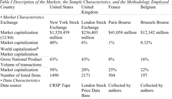
The sample consists of 1591 common stocks from four countries: 782 stocks traded on the New York Stock Exchange (NYSE), 527 stocks traded on the London Stock Exchange (LSE), 112 stocks traded on the Paris Stock Exchange, (PSE), and 170 stocks traded on the Brussels Stock Exchange (BSE). Comparative statistics on the four exchanges are given in Table I. The world's largest equity market is the NYSE, representing forty percent of the world's equity capitalization. One of the world's smallest is the BSE, representing one third of one percent of the world's equity capitalization. As a percentage of GNP, the NYSE and the LSE are about the same size (forty-three percent of GNP); the PSE and the BSE are considerably smaller. The European exchanges are not just smaller than their U.S. counterpart, but they are also considerably less active, as indicated by the significantly lower ratio of trading volume to market capitalization in London, Paris, and Brussels compared with New York. Finally, note the sharp decline in the average market capitalization across exchanges: from over $1 billion per firm on the NYSE to less than $63 million per firm on the BSE. Also, it is worth pointing out that the ten largest Belgian firms represent fifty-two percent of the total market capitalization on the BSE, whereas the ten largest U.S. firms represent only fifteen percent of the total market capitalization on the NYSE.
B. The Data
A general description of the sample properties and the methodology employed to estimate the risk premia are given in Table I. For all markets, the data begin in January 1969 and end in December 1983, thus yielding 180 monthly returns for each stock in the sample. The source of the data for U.S.
common stocks is the tape of the Center for Research in Security Prices (CRSP tape); for U.K. common stocks, it is the London Stock Price Data Base (Smithers [26, 27]).
Table I Description of the Markets, the Sample Characteristics, and the Methodology Employed
Country United States United
Kingdom
France Belgium
• Market Characteristics
Exchange New York Stock London Stock Paris Bourse Brussels Bourse
Exchange Exchange Market capitalization (12/84) $1,529,459 million $236,403 million $41,058 million $12,342 million Market capitalization World capitalizationa 40% 6% 1% 0.32% Market capitalization
Gross National Product 43% 43% 8% 16%
Volume of transactions
Market capitalization 50% 20% 25% 22%
Number of listed firms 1490 2171 504 197
• Data Characteristics
Data source CRSP Tape London Stock
Price Data Base Collected by authors Collected by authors
Data begin on January 1969 January 1969 January 1969 January 1969
Data end on December 1983 December
1983
December 1983 December 1983 Number of common
stocks
782 527 112 170
Market, index (including dividend yields) Equally weighted (from the CRSP Tape) Equally weighted (using the 527 stocks) Equally weighted (using the 112 stocks) Equally weighted (using the 170 stocks) • Return Characteristics
Length Monthly Monthly Monthly Monthly
Number 180 months 180 months 180 months 180 months
Definition Log of price
relatives adjusted for dividends Log of price relatives adjusted for dividends Log of price relatives adjusted for dividends Log of price relatives adjusted for dividends • Beta Characteristics
Number of estimated betasb 11,730 7905 1680 2550
Percent significantly different from zeroc
66% 58% 69% 44%
• Fama-MacBeth Methodology
Number of portfoliosd 20 20 20 20
Number of stocks per portfolio 40,39, •••,39, 40 30,26, •••,26, 29 6,5, •••,5,6 13,8, •••,8,
13 Length of portfolio construction
period
12 months 12 months 12 months 12 months
Length of beta-estimation period 12 months 12 months 12 months 12 months
Length of testing periode 12 months 12 months 12 months 12 months
Updating of portfolio construction period
Every year Every year Every year Every year
Updating of risk-estimation period Every year Every year Every year Every year
Total number of estimated monthly 156 (from Jan. '7 1 to 156 (from Jan. '71 to 156 (from Jan. '71 to 156 (from Jan. '71 to
parameters (γ0, γ1) Dec. '83) Dec. '83) Dec. '83) Dec. '83)
a Based on a world equity capitalization of $3,805 billion.
b Using one year of monthly observations; the reported number equals 15 years times the number of stocks.
c At the 0.05 level of significance (see footnote 12).
d Portfolios are formed with stocks ranked according to their beta values. e Cross-sectional regressions are run for every month of the year.
Prices and dividends for French and Belgian common stocks were collected by the authors. Common stocks that did not have a recorded end-of-month price were eliminated from the sample.5
C. The Properties of the Four Domestic Market Indexes
The domestic stock market indexes used in this study are equally weighted averages of common stock returns including dividend payments. In the case of the United States, we used the index given in the CRSP tape. For each of the three European markets, the average is that of the domestic common stocks in the sample.6 Monthly returns are calculated as logarithms of price relatives adjusted for dividend payments.7
Since one of the objectives of this paper is to investigate the relationship between the pattern of risk-premium seasonality and the pattern of return seasonality, we begin with an examination of the behavior of the month-to-month mean returns of the stock market index of each of the four countries in our sample. The results are summarized in Table II.
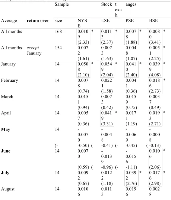
There is a significantly positive January seasonal in the stock market returns of the four countries. But the United States is the only country where returns are significantly positive only in January. In the United Kingdom, there is an April seasonal and, in France, a July seasonal.8 In Belgium, stock returns are significantly positive in February, April, June, and July, in addition to January. A Kruskal-Wallis nonparametric test shown at the bottom of Table II indicates that the hypothesis that the monthly mean returns are equal is rejected at the ten percent or less significance level only in the case of France9 and Belgium.10
Table II Month-to-Month Mean Stock Market Returns and Kruskal-Wallis Tests of Equality of Mean Returns from January 1970 to December 1983; Equally Weighted Indices for the New York, London, Paris, and Brussels Stock Exchangesa
Sample Stock t
exc h
anges
Average return over size NYS
E
LSE PSE BSE
All months 168 0.010 9 * 0.011 3 * 0.007 8 * 0.008 0 * (2.33) (2.37) (1.88) (3.41)
All months except January 154 0.007 2 0.007 3 0.004 8 0.005 1 * (1.61) (1.63) (1.07) (2.25) January 14 0.050 8 * 0.054 9 * 0.041 0 * 0.039 9 * (2.10) (2.04) (2.40) (4.08) February 14 0.007 8 0.022 1 0.004 1 0.018 6 * (0.74) (1.58) (0.36) (2.73) March 14 0.015 1 0.007 3 0.015 9 0.003 7 (0.94) (0.42) (0.75) (0.49) April 14 0.005 7 0.041 9 * 0.017 1 0.019 3 * (0.36) (3.31) (1.19) (2.71) May 14 -0.007 0 -0.004 8 -0.006 9 -0.000 8 (- -0.50) ( -0.41) (- -0.45) ( -0.13) June 14 0.007 0 -0.013 9 -0.015 6 0.010 6 * (0.59) ( -0.96) (- -1.11) (2.06) July 14 0.009 2 0.012 2 0.039 2 * 0.017 6 * (0.67) (1.18) (2.76) (2.98) August 14 0.010 6 0.011 3 0.019 6 0.002 8
(0.66) (0.83) (1.52) (0.36) September 14 0.003 1 -0.010 4 -0.004 0 -0.009 4 (0.23) ( -0.52) (- -0.21) ( -1.17) October 14 -0.009 1 -0.000 7 -0.017 6 -0.014 8 * (- -0.42) ( -0.06) (- -1.24) ( -2.48) November 14 0.022 5 0.000 6 -0.002 7 -0.007 0 (1.22) ( -0.029 ) (- -0.22) ( -0.98) December 14 0.014 8 0.016 2 0.003 7 0.015 8 (1.12 9) (1.06) (0.41) (1.58) K-W test: s tatisticsb 8.45 16.16 17.53 33.93 K-W test: p robability 0.672 8 0.135 2 0.093 2 0.000 4 a t-Statistics are in parentheses. They are computed aswith n = sample size. b See footnote 10 in the text for an explanation. * Significant at the 0.05 level.
Using tests based on a dummy-variable regression, we could not reject the hypothesis that the January mean returns in the four countries differ from the mean returns during the rest of the year. Likewise, we could not reject the hypothesis that the April mean returns in the U. K. differ from the mean returns during the rest of the year.11
D. The Return Properties of the Twenty Domestic Portfolios
To find out whether portfolios' mean returns exhibit monthly seasonalities similar to those observed in the mean returns of the stock market indexes, we examined the behavior of the month-to-month mean returns of the twenty portfolios we constructed for each of the four countries and compared them with the pattern of month-to-month mean returns of the corresponding four stock market indexes. We found that the pattern of seasonalities in the portfolios' mean returns is similar to that observed in the stock market indexes of the four countries. There is a January seasonal in the four countries. In the United States, eight out of the twenty portfolios have significantly positive mean returns in January, including the highest and lowest risk portfolios. Not a single portfolio was found in the United States with a significant mean return from February to December. In the United Kingdom, the April seasonal "dominates" the January seasonal. All twenty portfolios have mean returns that are significantly different from zero in April, whereas only nine out of twenty have significant mean returns in January. During the other ten months of the year, only February has portfolios with significant mean returns. In France, there is a July seasonal that "dominates" the January seasonal; fourteen out of twenty portfolios have mean returns that are significantly different from zero in July, but only eight out of twenty have significant mean returns in January. Finally, in Belgium, the January seasonal "dominates" all other months, with eighteen out of twenty portfolios having mean returns significantly different from zero.
E. The Methodology
To estimate each month's risk premium, we use the Fama and MacBeth [8] methodology. We run the regression
y0t and the slope coefficient y1t in regression (1), we proceeded as follows.
Using the first year of monthly returns, we estimated the betas of the 1591 common stocks in the sample based on their respective domestic market indexes.12
We then ranked each country's stocks from the highest to lowest estimated beta and constructed twenty equally weighted domestic portfolios, the first portfolio containing the securities with the highest risk. The number of securities in each portfolio is given in Table I.13
We then used the second year of monthly returns to estimate the securities' systematic risks (betas). The estimated betas of each portfolio were then calculated by taking the arithmetic average of the betas of the individual stocks making up the portfolio. Finally, we tested the relationship between portfolio returns and risk over the third year of monthly returns (the test period). For each month of the twelve-month test period, we calculated the realized return of each of the twenty domestic portfolios. These twenty portfolio returns were then cross-sectionally regressed on estimated betas according to regression (1). Recall that risk is estimated over the preceding twelve-month risk-estimation period. From the twelve cross-sectional regressions, we obtained twelve monthly estimates of γ0 and γ1: one for each month of the year.
The entire procedure was then repeated using the second year of monthly data to construct portfolios, the third year of monthly data to estimate risk, and the fourth year of monthly data to estimate the monthly relationship between realized returns and risk. Dropping one year of yearly data and adding a new one, we kept on repeating the entire procedure until we reached the year 1983. This approach provided a total of 156 monthly estimates of γ0 and γ1: thirteen estimates for each of the twelve months of the year (from January 1971 to December 1983).
II. Empirical Evidence
A. The Risk-Return Relationship over the Entire Thirteen- Year Period
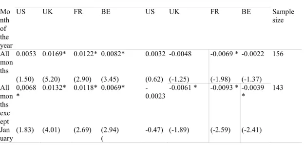
On the upper part of Table III, we report the average values, over the entire thirteen-year period (156 months) from January 1971 to December 1983, of the intercept and slope coefficients of the regression of realized portfolio returns on systematic risk.
Table III Average Values of the Fama and MacBeth Estimates of the Intercept and Slope Coefficients for Each Month of the Year from January 1971 to December 1983 for the Regression Rpt = yot + y1tβp + µpt(a) Mo nth of the year US UK FR BE US UK FR BE Sample size All mon ths 0.0053 0.0169* 0.0122* 0.0082* 0.0032 -0.0048 -0.0069 * -0.0022 156 (1.50) (5.20) (2.90) (3.45) (0.62) (-1.25) (-1.98) (-1.37) All mon ths exc ept 0,0068 * 0.0132* 0.0118* 0.0069* -0.0023 -0.0061 * -0.0093 * -0.0039 * 143 Jan uary (1.83) (4.01) (2.69) (2.94) ( -0.47) (-1.89) (-2.59) (-2.41)
Jan uary -0.0108 0.0464* 0.0171 0.0234* 0.0632 * 0.0091 0.0193 0.0162 * 13 (-0.91) (3.94) (1.09) (1.91) (2.46) (0.40) (1.21) (2.63) Feb ruar y -0.0095 0.0282* 0.0104 0.0174* 0.0115 -0.0038 -0.0068 0.0003 13 (-1.08) (2.83) (0.89) (2.10) (0.68) (-0.35) (-0.61) (0.05) Mar ch -0.0068 0.0181 0.0282 0.0048 0.0227 -0.0099 -0.0157 -0.0037 13 (-0.48) (1.73) (1.43) (1.12) (0.95) (-0.68) (-1.01) (-0.48) Apr il 0.0059 0.0282* 0.0207 0.0206* 0.0089 0.0220 * -0.0026 -0.0026 13 (0.38) (2.11) (1.48) (2.24) (0.65) (1.98) (-0.22) (-0.53) Ma y 0.0054 0.0236* 0.0111 0.0021 -0.0085 -0.0211 * -0.0194 * -0.0032 13 (0.44) (2.47) (0.75) (0.32) ( -0.63) (-3.33) (-1.91) (-0.95) Jun e 0.0247 * 0.0111 0.0006 0.0229* -0.0160 -0.0287 * 0.0179 -0.0140 * 13 (2.68) (1.21) (0.03) (3.26) ( -1.29) (-1.96) (-1.64) (-2.68) July -0.0099 0.0084 0.0407* 0.0103* 0.0096 0.0013 -0.0057 0.0030 13 (-0.87) (0.90) (3.50) (1.89) (0.52) (0.12) (-0.53) (0.56) Aug ust 0.0101 0.0000 0.0192 0.0105 -0.0070 0.0116 -0.0017 -0.0104 * 13 (0.64) (-0.00) (1.53) (1.24) ( -0.45) (1.25) (-0.17) (-2.23) Sept emb er 0.0092 -0.0059 -0.0119 -0.0030 -0.0167 -0.0088 -0.0056 -0.0089 * 13 (1.02) (-0.39) (-1.12) (-0.36) ( -1.88) (-0.66) (0.39) (-2.13) Oct ober 0.0265 0.0140 -0.0173 -0.0079 -0.0362 -0.0159 -0.0067 -0.0106 * 13 (1.70) (1.65) (-1.01) (-1.61) ( -1.68) (-1.39) (-0.45) (-1.88) Nov emb er 0.0047 0.0125 0.0061 -0.0122* 0.0133 -0.0086 0.0101 0.0040 13 (0.42) (0.97) (0.46) (-1.82) (0.90) (-0.67) (-0.98) (1.02) Dec emb er 0.0147 0.0182 0.0210* 0.0097 -0.0067 -0.0045 -0.0212 * 0.0031 13 (1.55) (1.81) (1.91) (0.98) (- -0.57) (-0.34) (-1.88) (0.51)
(a) t-Statistics are given in parentheses below the average values; refer to Table I for details on the sample properties and methodology. * Significant at the 0.05 level.
A look at the t-statistics for the estimated average risk premium indicates that it is not
significantly different from zero, except for the case of France, where it is negative. This means that investors in stocks trading in the United States, the United Kingdom, and Belgium were not
compensated with higher average returns for bearing higher levels of risk over the thirteen-year sample period.14 Investors in stocks trading on the Paris Stock Exchange were actually penalized rather than rewarded. They received below-average rates of return for holding stocks with above-average levels of risk. It appears, then, that the absence of a positive relationship between average returns and risk in the seventies and early eighties is not a characteristic unique to U.S. common stocks; it is also observed in
the United Kingdom, France, and Belgium.15 Finally, note that the average intercept coefficient is
B. January versus the Rest of the Year
The fact that the average risk premium is not different from zero over the thirteen-year sample period does not rule out the possibility that it may be different from zero over a particular month of the year. Tinic and West [28] report that, in the United States, the risk premium is actually positive in January and not significantly different from zero over the other eleven months. Our results for U.S. common stocks on the upper part of Table III point to the same conclusion. The average estimated monthly market risk premium is equal to 6.32 percent in January alone.16 It is not different from zero during the remaining eleven months.
Is this puzzling phenomenon also observed in European stock exchanges? In the case of Belgium, the risk premium is, like in the United States, significantly positive in January (1.62 percent). But, unlike the United States, the risk premium is significantly negative during the remaining eleven months (-.39 percent). What about the United Kingdom and France? We observe a positive January risk premium in both countries, but it is not significantly different from zero. Note, however, that in both countries the risk premium during the rest of the year is significantly negative, as in the case of Belgium. In the United Kingdom it is -.61 percent, and in France it is -.93 percent.17
It seems, then, that a significant positive January risk premium, similar to that observed in the United States, is only revealed in the case of Belgian common stocks. But this does not mean that the January risk premium does not differ from the average risk premium during the rest of the year in France and the United Kingdom. To test the hypothesis that the risk premium in January is equal to the average risk premium during the rest of the year, we run the regression
over our entire thirteen-year sample period (from January 1971 to December 1983). In the regression, y1t is the monthly estimate of the risk premium, and D2 is a dummy variable representing the rest of the year. (D2 equals one the rest of the year and zero in January.) The regression intercept a1 measures the difference between the average risk premium in January and the average risk premium during the remaining eleven months of the year. If the average risk premium in January is the same as the average risk premium during the rest of the year, the estimate of a2 will not be statistically different from zero. We found the following:
γ1tUS = 0.0632 - 0.0655 D2 (United States), (3.69) (-3.66) γ1tUκ = 0.0091 - 0.0152 D2 (United Kingdom), (0.69) (-1.10) γ1tFR = 0.0193 - 0.0285 D2 (France), (1.57) (-2.23)
γ1tBE = 0.0162 - 0.0201 D2 (Belgium). (2.98) (-3.54)
We can see that the estimate of a2 is negative and statistically different from zero only in the case of the U.S., French, and Belgian common stocks (where t-statistics, in parentheses, exceed -2.00). This means that, in the United States, France, and Belgium, the average risk premium from February to December (the rest of the year) is significantly smaller than the average risk premium in January.18 More important, however, is the fact that there is no significant January seasonal in the U.K. risk premium.19
C. Month-to-Month Estimates of the Risk Premium
The absence of a January seasonal in the U.K. risk premium does not rule out the presence of seasonality during some other months of the year. It is also possible that seasonality exists in months other than January in the United States, France, or Belgium. To find out whether this is indeed the case, we estimated the month-to-month average intercept and average slope coefficient (risk premium) of the risk-return relationship for the four countries in our sample. Our results are summarized on the lower part of Table III.
Turning first to the United Kingdom, we can see that, in April, the risk premium is significantly positive and equal to 2.20 percent. As a matter of fact, April is the only month of the year with a significantly positive risk premium. In May and June, the risk premia are significant but negative. The results for the United States and Belgium confirm that, in these two countries, the risk premium is significantly positive only in January. In France, there is a weak January seasonal. The January risk
premium is positive (1.93 percent) but not statistically significant. Note that, although not a single month of the year has a significant positive risk premium in France, January and September are the only months of the year with a positive (but insignificant) risk premium.
Turning to the intercept coefficient γ0, no consistent patterns emerge from the results summarized in Table III. For the United States, γ0 is significantly positive only in June. It is significantly positive in January, February, April, and May in the United Kingdom. In France, it is significantly positive in July and December. In Belgium, it is significantly positive in January, February, April, June, and July and significantly negative in November.
In order to test the hypothesis that the month-to-month risk premia (γ1) are equal, we run the regression over our entire thirteen-year sample period for the four countries in our sample. In regression (3), Dt are dummy variables representing each month of the year from February (t = 2) to December (t = 12). The regression intercept a1 measures the average risk premium in January, while the regression slopes at measure the difference between the average risk premium in January and the average risk premium in month t. As in the case of regression (2), a slope at that is statistically different from zero indicates that the average risk premium in month t is different from the average risk premium in January. We found that, in the United States, except for March, risk premia differ in January from all other months of the year. In the United Kingdom, only the June risk premium is different from the January risk premium. In France, the March, May, and June risk premia are different from the January risk premium, and, in Belgium, all months but July, November, and December have risk premia that differ from that of January.
To summarize, there is a strong positive January seasonal in the risk premium of U.S. and Belgian common stocks. There is no January seasonal in the risk premium of U.K. common stocks. It is replaced by an April seasonal. There is not a single month of the year with a significantly positive risk premium in France. The French January risk premium, however, is the year's largest.
D. Comparative Analysis of U.S. and European Risk Premia
We have shown that the seasonal behavior of the risk premia differs across the four countries in our sample. How significant are these differences in risk premia across the national stock markets? To answer this question we run the regression
for each month t of the year from January (t = 1) to December (t = 12). The dependent variable is the risk premium in month t for country i. (i = U.S. for the United States, i = 1 for the United Kingdom, i =2 for France, and i = 3 for Belgium.) The dummy variable Mt represents month t (Mt equals one in month t and zero otherwise), the dummy variable Dlt represents country i, and the dummy variable Sit is equal to Mt Dit. The regression coefficients have the following interpretation:
The intercept a0 is the average U.S. risk premium during the rest of the year (r). The slope a0* is the difference between the average U.S. risk premium in month t and the average U.S. risk premium during the rest of the year. We define this difference as the average excess risk premium in month t. Using this definition, the slope ai* is the difference between the average excess risk premium in country i and the average excess risk premium in the United States. Finally, the slope ai is the difference between the average risk premium during the rest of the year in country i and the average risk premium during the rest of the year in the United States.
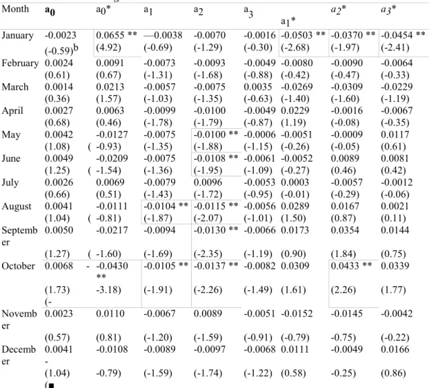
Regression (4) was run twelve times, once for every month of the year (t = 1, • • •, 12). The estimated regression coefficients and their corresponding t-statistics are given in Table IV. The a0 column indicates that the average U.S. risk premium during the rest of the year is never significant, regardless of which month of the year is excluded to obtain the rest of the year. The a0* column indicates that the
average U.S. excess risk premium is significantly positive in January (6.55 percent) and significantly negative in October (-4.30 percent). That is, the average U.S. risk premium is significantly larger in January than the rest of the year and significantly smaller in October than the rest of the year. (The average October risk premium is equal to -3.62 percent, as shown in Table III.) The a1 column indicates that the average risk premium during the rest of the year in the United Kingdom is significantly smaller than that in the United States if we exclude April, August, or October from the twelve months of the year. The a2 column indicates that the average risk premium during the rest of the year in France is also significantly smaller than that in the United States.
Table IV Test of the Hypothesis of Equal Risk Premia (γ1) in Month t and the Rest of the Year (r) across Countries (i = 1 is the U.K., i = 2 is France, i = 3 is Belgium) Estimated from January 1970 to December 1983 with the Regressiona
Month a0 a0* a1 a2 a
3
a1* a2* a3*
January -0.0023 0.0655 ** —0.0038 -0.0070 -0.0016 -0.0503 ** -0.0370 ** -0.0454 ** (-0.59)b (4.92) (-0.69) (-1.29) (-0.30) (-2.68) (-1.97) (-2.41) February 0.0024 0.0091 -0.0073 -0.0093 -0.0049 -0.0080 -0.0090 -0.0064 (0.61) (0.67) (-1.31) (-1.68) (-0.88) (-0.42) (-0.47) (-0.33) March 0.0014 0.0213 -0.0057 -0.0075 0.0035 -0.0269 -0.0309 -0.0229 (0.36) (1.57) (-1.03) (-1.35) (-0.63) (-1.40) (-1.60) (-1.19) April 0.0027 0.0063 -0.0099 -0.0100 -0.0049 0.0229 -0.0016 -0.0067 (0.68) (0.46) (-1.78) (-1.79) (-0.87) (1.19) (-0.08) (-0.35) May 0.0042 -0.0127 -0.0075 -0.0100 ** -0.0006 -0.0051 -0.0009 0.0117 (1.08) ( -0.93) (-1.35) (-1.88) (-1.15) (-0.26) (-0.05) (0.61) June 0.0049 -0.0209 -0.0075 -0.0108 ** -0.0061 -0.0052 0.0089 0.0081 (1.25) ( -1.54) (-1.36) (-1.95) (-1.09) (-0.27) (0.46) (0.42) July 0.0026 0.0069 -0.0079 0.0096 -0.0053 0.0003 -0.0057 -0.0012 (0.66) (0.51) (-1.43) (-1.72) (-0.95) (-0.01) (-0.29) (-0.06) August 0.0041 -0.0111 -0.0104 ** -0.0115 ** -0.0056 0.0289 0.0167 0.0021 (1.04) ( -0.81) (-1.87) (-2.07) (-1.01) (1.50) (0.87) (0.11) Septemb er 0.0050 -0.0217 -0.0094 -0.0130 ** -0.0066 0.0173 0.0354 0.0144 (1.27) ( -1.60) (-1.69) (-2.35) (-1.19) (0.90) (1.84) (0.75) October 0.0068 - -0.0430 ** -0.0105 ** -0.0137 ** -0.0082 0.0309 0.0433 ** 0.0339 (1.73) (- -3.18) (-1.91) (-2.26) (-1.49) (1.61) (2.26) (1.77) Novemb er 0.0023 0.0110 -0.0067 0.0089 -0.0051 -0.0152 -0.0145 -0.0042 (0.57) (0.81) (-1.20) (-1.59) (-0.91) (-0.79) -0.75) (-0.22) Decemb er 0.0041 - -0.0108 -0.0089 -0.0097 -0.0068 0.0111 -0.0049 0.0166 (1.04) (■ -0.79) (-1.59) (-1.74) (-1.22) (0.58) -0.25) (0.86)
aThe dummy variable Mt represents month t, Dit represents country i, and Sit = Mt . Dit. The
regression coefficients are interpreted as follows:
b t-Statistics are in parentheses. ** Significant at the 0.05 level.
This is the case if we exclude April, May, June, August, September, October, or December from the twelve months of the year. Finally, note that we cannot reject the hypothesis that the average risk premia during the rest of the year are equal in the United States and Belgium (the a3 column).
The last three columns indicate that the average excess risk premium in January is significantly smaller in the United Kingdom, France, and Belgium than in the United States. For the other months of the year, there are no significant differences across stock exchanges, except in October, where the French average excess risk premium is significantly larger than that in the United States.
E. Return Seasonality versus Risk-Premium Seasonality
Let us summarize our results regarding the patterns of return seasonality and risk-premium seasonality in the four countries in our sample. In the United States, there is a positive January seasonal in
portfolios' returns, as well as a January seasonal in the market risk premium. More important is the fact that January is the only month of the year for which these two phenomena are significant. In other words, in the United States, portfolios' returns and the market risk premium are both significantly positive only in January. Over every one of the other eleven months, neither portfolios' returns nor the market risk premium are different from zero. In light of this result, we may be tempted to conclude that the January seasonal in the risk premium may be nothing but a reflection of the January seasonal in stock returns and that both phenomena may simply be the manifestations of the same underlying factors. However, the evidence from the three European countries indicates that the pattern of return seasonality can differ from the pattern of risk-premium seasonality.
What is the analytical relationship between return seasonality and estimated risk-premium seasonality? Suppose that portfolios' mean returns (Rp ) exhibit seasonality only in month t ; the rest of the year, the monthly returns are equal to µp. We can write
where λpt is the excess return earned by portfolio p in month t. Assume that the estimated systematic risk of portfolio p (βp) does not exhibit any seasonality;20 then, the estimated monthly risk premium in any month other than the seasonal month t is
and the estimated risk premium in month t becomes
It follows from equations (5) and (6) that the seasonality in the risk premium is related to the seasonality in portfolio returns only if beta does not exhibit any seasonality and cov(λpt, βp) is different from zero. And the absence of seasonality in portfolio returns (λpt = 0) will imply no seasonality in the risk premium (γ1t =) if beta does not exhibit any seasonality.
In other words, if beta is not seasonal, then cov(λpt, βP) different from zero in month t implies that, over that month, we should observe both return seasonality and risk-premium seasonality.
To examine the empirical validity of the above argument, we estimated the second term in equation (6) in the following manner. For each country, we calculated the term λpt for each one of the twenty portfolios over each month of the year from January 1970 to December 1983 by taking the difference between the return of portfolio p in month t (Rpt) and the mean return of portfolio p over the twelve months of the year. We then ran 168 (fourteen years times twelve months) cross-sectional regressions of λpt on βp (twenty observations), where the latter term is the portfolio's beta estimated over the preceding year.21 We have
where αt is an estimate of the slope coefficient cov(λpt, βp)/var(βp).
In Table V, we present the average values of αt from January (t = 1) to December (t = 12) with their corresponding t-statistics for the four countries in our sample.
In the case of the United States, the evidence in Table V is in line with the analytical argument; the average value of the second term in equation (6) is significantly positive only in January. This is consistent with the fact that, in the United States, we have a return seasonal and a risk-premium seasonal only in January. (Compare the results in Table II with those in Table III.) In other words, in the United States and over our sample period, return seasonality is the probable cause of risk-premium seasonality.
In the case of the United Kingdom, the average value of the second term in equation (6) is significantly positive only in April. Again, this is consistent with the fact that, in the United Kingdom, we have a return seasonal and a risk-premium seasonal only in April. (Compare the results in Table II with those in Table III.) But the average value of the second term in equation (6) is not statistically significant in January. Hence, despite the presence of a January seasonal in the U.K. stock returns, we do not observe a January seasonal in the estimated U.K. risk premia.
Table V Average Values of the Estimates of the Slope Coefficient for Each Month of the Year from January 1970 to December 1983 (Fourteen Observations for Each Month of the Year) for the
Regressiona λpf = αt* + αt βp + ept
Month United States United Kingdom France Belgium
January 0.0628 * 0.0240 0.0299 0.0312 * (2.17) (1.09) (1.74) (2.35) February 0.0097 0.0128 -0.0008 0.0046 (0.68) (0.99) (-0.06) (0.81) March 0.0129 -0.0034 0.0056 -0.0099 (0.63) (-0.19) (0.35) (-1.20) April -0.0084 0.0248 * 0.0124 0.0118 * (—0.57) (1.98) (0.87) (1.99) May -0.0214 -0.0198 -0.0218 -0.0129 (-1.78) (-1.71) (-1.33) (-1.72) June -0.0159 -0.0314 0.0306 0.0048 (—1.57) (—1.63) (-1.75) (0.85) July 0.0061 0.0223 0.0237 0.0124 (0.33) (0.12) (1.35) (1.62) August 0.0022 0.0072 0.0100 -0.0018 (0.14) (0.73) (0.83) (-0.22) September —0.0047 -0.0199 0.0124 -0.0130 * (-0.29) (-1.19) (0.52) (-2.02) October -0.0383 -0.0135 -0.0124 -0.0254 * (-1.72) (-0.71) (-0.56) (-3.06) November 0.0104 -0.0131 -0.0074 -0.0006 (0.68) (—0.06) (-0.48) (-0.05) December -0.0156 0.0182 -0.0210 -0.0013 (-1.09) (1.24) (-1.15) (-0.10)
a it-Statistics are given in parentheses below the average values. * Significant at the 0.05 level.
In France, the average value of the second term in equation (6) is never significantly different from zero. Hence, we cannot find a single month of the year that exhibits both return seasonality and risk-premium seasonality. (Compare the results in Table II with those in Table III.) Belgium is the only country that does not fully comply with the above argument according to which we should observe return seasonality and risk-premium seasonality over a given month only if the average value of the second term in equation (6) is different from zero. The evidence is consistent with the argument in January and October. It is not in April and September. (Compare the results in Table II with those in Table III.) Seasonality in the estimated Belgian beta coefficients may be the cause of this
phenomenon.22
III. Summary and Conclusion
In this paper, we have examined the monthly behavior of the CAPM-based risk premia in the United States, the United Kingdom, France, and Belgium. These risk premia were estimated according to the Fama and MacBeth [8] methodology. We have seen that equity markets differ widely in terms of size and activity among these countries. The world's largest and most active exchange is the NYSE; one of the world's smallest and least active is the Brussels Stock Exchange. Despite these differences, our empirical evidence reveals a common characteristic across the four stock exchanges: the presence of persistent seasonalities in these markets' risk premia and stock returns. In the United States and Belgium, the relationship between average portfolio returns and their corresponding systematic risk is significantly positive only in January. This positive January seasonal is not observed in the United Kingdom. It is replaced by an April seasonal, the only month of the year during which the relationship between average portfolio returns and systematic risk is significantly positive on the London Stock Exchange. In France, the January risk premium is positive and larger than the risk premium during the rest of the year, but it is not significantly different from zero. Contrary to the case of the United States, where the relationship between the average portfolio returns and systematic risk is not significantly
different from zero the rest of the year, it is, on average, significantly negative during the other eleven months of the year in the three European countries in our sample. We have also found that the January excess risk premium (the January premium less the premium during the rest of the year) is significantly larger in the United States than in the three European countries in our sample. During the rest of the year, however, the European risk premia do not differ significantly from the U.S. risk premium. Finally, in order to find out whether the monthly risk premium seasonal is simply a reflection of the monthly return seasonal observed in the four countries, we compared, in each country, the pattern of risk-premium seasonality with the pattern of return seasonality. Although a perfect correspondence between these patterns exists in the United States, it is not the case in the United Kingdom, France, and Belgium. A possible explanation of this phenomenon is presented in the previous section.
Notes
1 There is a growing literature dealing with the issue of seasonality in the monthly returns of stock market indexes around the world. For the case of Canada see Berges, McConnell, and Schlarbaum [2], as well as Tinic, Barone-Adesi, and West [30]. For the Australian evidence see Officer [21] and Brown, Keim, Kleidon, and Marsh [4]. For the case of Japan see Jaffe and Westerfield [14] and Kato and Schallheim [15]. The evidence for European countries is found in Hamon [10] for the case of France, Reinganum and Shapiro [22], Dimson and Marsh [7], Beckers, Rosenberg, and Rudd [1], and Levis [17] for the case of the United Kingdom, Wahlroos and Berglund [31] for the case of Finland, van den Bergh and Wessels [3] for the case of the Netherlands, and Santesmases [25] for the case of Spain.
2 For the period January 1935 to December 1982, Tinic and West [28] report that the Fama-MacBeth average estimate of the market risk premium is 0.0470 in January with a t-statistic of 4.63. For the rest of the year it is 0.0038, with a i-statistic of 1.41. When all months are considered, the market risk premium is .0074, with a t-statistic of 2.80. Similar qualitative results are reported over shorter periods. 3 The evidence for the case of the United Kingdom is found in Corhay, Hawawini, and Michel [6], for the case of France in Hawawini, Michel and Viallet [13], and for the case of Belgium in Hawawini and Michel [11], The British data do not support the CAPM over a twenty-seven-year period from January 1957 to December 1983. The risk-return relationship is negative but not significantly different from zero. The French data tend to support CAPM, but the risk-return relationship is persistently negative. The Belgian data are consistent with the CAPM, with the risk-return relationship positive over the eight-year period from December 1966 to November 1974 and negative over the four-year period from December 1976 to November 1980.
4 According to the tax-loss selling hypothesis, as the end of the fiscal year approaches, investors can reduce their taxes by selling the stocks on which they lost money during the year. In doing so, they realize capital losses that are deductible from their taxable income. The sale of securities at the end of the fiscal year depresses prices, which recover at the beginning of the next fiscal year as stocks move back toward their equilibrium value. For countries with a fiscal year ending in December (United States, France, and Belgium), this trading implies that mean returns in December will be smaller than in the other months of the year and that mean returns in January will be significantly larger. In the United Kingdom, individuals close their fiscal year at the beginning of April, but corporations and partnerships may select the last day of December as the end of their fiscal year. Hamon [10] concludes that the behavior of French stock returns is consistent with the tax-loss selling hypothesis. Reinganum and Shapiro [22] find that the behavior of British stock returns is consistent with the tax-loss selling hypothesis, and Beckers, Rosenberg, and Rudd [1] conclude that their statistical analysis of the British data provides weak support for the tax-loss selling hypothesis.
5This criterion may introduce a slight "survivalship" bias since the sample contains only the securities of those firms that were successful over the entire period.
6 For the case of the United Kingdom, France, and Belgium, the use of other indexes, some of which are value weighted, did not materially affect the results.
7 Note that, for returns less than ten percent, the logarithm of wealth relatives is equal to the logarithm of one plus the rate of return, which is in turn approximately equal to the rate of return. We have
log((Pt + Dt )/Pt-1) = log(1 + Rt) ≈ Rt .8 The July seasonal may be attributed partly to the fact that, in France, roughly two thirds of all dividend payments occur in July (Hamon [10]). Litzenberger and Ramaswamy [19, 20] have shown that shareholders' expected returns are positively related to dividend yields. It follows that, in months when dividends are paid, average returns should be higher, relative to those months in which no dividends are paid-hence, the observed July seasonal in France.
9 Our results do not seem to confirm those reported in Gultekin and Gultekin [9], except for the case of Belgium. They found that, in France, the month-to-month returns do not differ at the ten percent level of significance and that, in the United Kingdom, the month-to-month returns do differ at the ten percent level of significance. We found the opposite; in France, month-to-month returns are significantly different, and, in the United Kingdom, they are not. It follows that the seasonal behavior of stock market indexes is sensitive to the nature of the index and the period of time over which seasonality is examined.
10 The Kruskal-Wallis test is nonparametric and tests the null hypothesis that the month-to-month average mean returns are equal against the alternative that they are not. It is distributed approximately as a chi-square distribution with eleven degrees of freedom. The probability values given at the bottom of Table II are values for the probability that the reported corresponding chi-square statistics would be realized if the average values of the monthly mean returns were equal. The critical value for the chi-square distribution with eleven degrees of freedom at the ten percent level of significance is 17.27. 11For example, for the case of the January seasonal, we found the following set of regressions:
RtUS = 0.0508 - 0.0435 D2 (3.20) (—2.62)
RtUK = 0.0549 — 0.0476 D2 (3.39) (-2.81)
where Rt represents mean returns and D2 is a dummy variable representing the rest of the year. The intercepts are the January mean returns, and the slopes are the differences between mean returns during the rest of the year and the mean returns in January. The t-statistics (in parentheses) clearly indicate that, in all four countries, the market returns in January differ from those during the rest of the year. 12 Note that we have only fifteen years of data. We use one year of data to construct portfolios, one year to estimate beta coefficients, and the remaining thirteen years to estimate the risk-return relationship. (See the lower part of Table I.) The reason we only use twelve monthly return
observations (one year) to estimate betas is to save as many observations as possible to test the model. But twelve observations may not be sufficient to estimate betas reliably. Turning to Table I, note that the percentage of estimated betas that are significantly different from zero at the 0.05 level is sixty-six percent in the United States, fifty-eight percent in the United Kingdom, sixty-nine percent in France, and forty-four percent in Belgium. These percentages did not increase significantly when we lengthened the beta estimation period to either twenty-four or thirty-six months. Also, the average t-statistics did not increase significantly. Hence, lengthening the beta estimation period would have reduced the model estimation period without significantly increasing the reliability of beta estimates. Finally, it should be pointed out that the percentage of beta estimates that are not significantly different from zero is particularly large in the five portfolios with the lowest beta coefficients. The ten portfolios with the highest betas have a percentage of significant betas ranging from ninety-six to seventy-nine percent.
13 The "errors-in-the-variable" problem may be particularly serious in risk premia estimates in European stock markets due to, first, the small number of return observations used to estimate beta coefficients (see footnote 12) and, second, the small number of stocks in each portfolio (particularly in France and Belgium). As a result, comparisons across stock markets may not be statistically reliable and should be interpreted cautiously. Note, however, that Hawawini, Michel, and Corhay [12] have shown that the stability and reliability of Belgian beta coefficients can be greatly improved by constructing portfolios containing a very small number of securities. (For example, five stocks may be sufficient.)
14 We have shown that this result holds even if risk is measured by the variance of total returns (total risk) instead of systematic risk. The reason we rerun the regressions with variance as the measure of
risk is that, in smaller markets, investors may not be well diversified. In this case, the variance may play a more important role than systematic risk in pricing securities (Levy [18]). It is possible, of course, that variance may simply be acting as a proxy variable for systematic risk.
15 This result may be interpreted as some evidence of international integration among these markets. 16 Our results are similar to those reported by Tinic and West [28]. They found an average estimated monthly risk premium of 6.09 percent in January, with a t-statistic of 2.64 for the period January 1969 to December 1982.
17 Interestingly, we found that a significant positive January seasonal is observed in the United States, the United Kingdom, and Belgium when risk is measured as variance. Note that, in the case of the United Kingdom, there is a January seasonal when variance is the measure of risk but no January seasonal when systematic risk is the measure of risk.
18 We have used the same technique to find out whether the average intercept term in the risk-return relationship is also different in January from its average value during the rest of the year. We found a significant positive January seasonal only in the United Kingdom and Belgium.
19 We run a regression similar to regression (2) for the case of the United Kingdom in order to compare the average risk premium in April to the average risk premium during the rest of the year. We found the following:
γ1t = .0220 - .0292 D2. (1.67) (2.13)
Since the regression slope measures the difference between the average risk premium in April and the average risk premium during the remaining eleven months, we can conclude that the average April risk premium is significantly different from the average risk premium during the rest of the year.
20 Preliminary work on our sample indicates that this may be the case for the four countries in the sample, with some exceptions in the case of Belgium. In general, we could not reject the hypothesis of beta invariance when betas were estimated with only January data, February data, etc., in the case of the United States, the United Kingdom, and France. In this respect see Corhay, Hawawini, and Michel [5].
21 Note that the methodology we use to estimte at is the Fama and MacBeth [8] methodology we
employed to estimate the risk premium. 22 See footnote 20.
REFERENCES
[1]. S. Beckers, B. Roenberg, and A. Rudd. "The January or April Effect: Seasonal Evidence from the United Kingdom." Working Paper, BARRA, Berkeley, California, March 1983.
[2]. A. Berges, J. McConnell, and G. Schlarbaum. "The Turn of the Year in Canada." Journal of Finance 39 (March 1984), 185-92.
[3]. W. van den Bergh and R. Wessels. "Seasonality of Individual Stock Returns: Recent Empirical Evidence for the Amsterdam Stock Exchange." Working Paper, Presented at the 10th Annual Meeting of the European Finance Association, Fountainebleau, France, September 1983.
[4]. P. Brown, D. Keim, A. Kleidon, and T. Marsh. "Stock Return Seasonalities and the Tax-Loss Selling Hypothesis: Analysis of the Arguments and Australian Evidence." Journal of Financial Economics 12 (June 1983), 105-27.
[5]. A. Corhay, G. Hawawini, and P. Michel. "Risk-Premia Seasonality in US and European Equity Markets." Working Paper, INSEAD, Fontainebleau, France, February 1986.
[6]. A. Corhay, G. Hawawini, and P. Michel. "The Pricing of Equity on the London Stock Exchange: Seasonality and Size Premium." In E. Dimson (ed.), Stock Market Anomalies. Cambridge University Press, 1987.
[7]. E. Dimson and P. Marsh. "The Impact of the Small Firm Effect on Event Studies and the Performance of Published UK Stock Recommendations." Working Paper, London Business School, March 1984.
[8]. E. Fama and J. MacBeth. "Risk, Return and Equilibrium: Empirical Tests." Journal of Political Economy 71 (May/June 1973), 607-36.
[9]. M. Gultekin and B. Gultekin. "Stock Market Seasonality: International Evidence." Journal of Financial Economics 12 (December 1983), 469-82.
[10]. J. Hamon. "The Seasonal Character of Monthly Returns on the Paris Bourse" (in French). Finance (the Journal of the French Finance Association) 7 (June 1986), 57-74.
[11]. G. Hawawini and P. Michel. "The Pricing of Risky Assets on the Belgian Stock Market." Journal
of Banking and Finance 6 (June 1982), 161-78.
[12]. G. Hawawini, P. Michel, and A. Corhay. "New Evidence on Beta Stationarity and Forecast for Belgian Common Stocks." Journal of Banking and Finance 9 (December 1985), 553-60.
[13]. G. Hawawini, P. Michel, and C. Viallet. "An Assessment of the Risk and Return of French Common Stocks." Journal of Business Finance and Accounting 10 (Autumn 1983), 333-50.
[14]. J. Jaffe and R. Westerfield. "Patterns in Japanese Common Stock Returns: Day of the Week and Turn of the Year Effects." Journal of Financial and Quantitative Analysis 20 (June 1985), 261-72. [15]. K. Kato and J. Schallheim. "Seasonal and Size Anomalies in the Japanese Stock Market." Journal of Financial and Quantitative Analysis 20 (June 1985), 243-60.
[16]. D. Keim. "Size-Related Anomalies and Stock Return Seasonality: Further Empirical Evidence." Journal of Financial Economics 12 (June 1983), 13-22.
[17]. M. Levis. "Are Small Firms Big Performers?" Investment Analyst 76 (April 1985), 21-27. [18]. H. Levy. "Equilibrium in an Imperfect Market: A Constraint on the Number of Securities in the Portfolio." American Economic Review 68 (September 1978), 643-58.
[19]. R. Litzenberger and K. Ramaswamy. "The Effect of Personal Taxes and Dividends on Capital Asset Prices: Theory and Empirical Evidence." Journal of Financial Economics 7 (June 1979), 163-95. [20]. R. Litzenberger and K. Ramaswamy. "The Effects of Dividends on Common Stock Prices: Tax Effects or Information Effects?" Journal of Finance 37 (March 1982), 429-43.
[21]. R. Officer. "Seasonality in Australian Capital Markets: Market Efficiency and Empirical Issues." Journal of Financial Economics 2 (June 1975), 29-51.
22]. M. Reinganum and A. Shapiro. "Taxes and Stock Return Seasonality: Evidence from the London Stock Exchange." Working Paper, Graduate School of Business, University of Southern California, Los Angeles, 1984.
[23]. R. Roll. "The Turn-of-the-Year Effect and the Return Premia of Small Firms." Journal of Portfolio Management 9 (Winter 1983), 18-28.
[24]. M. Rozeff and W. Kinney. "Capital Market Seasonality: The Case of Stock Returns." Journal of Financial Economics 3 (September 1976), 379-402.
[25]. M. Santesmases. "An Investigation of the Spanish Stock Market Seasonalities." Journal of Business Finance and Accounting 13 (Summer 1986), 267-76.
[26]. P. Smithers. "London Share Price Data Base." London Business School, February 1977. [27]. P. Smithers. "LBS Financial Database Manual." London Business School, March 1980. [28]. S. Tinic and R. West. "Risk and Return: January versus the Rest of the Year." Journal of Financial Economics 13 (December 1984), 561-74.
[29]. S. Tinic and R. West. "Risk, Return, and Equilibrium: A Revisit." Journal of Political Economy 94 (February 1986), 126-47.
[30]. S. Tinic, G. Barone-Adesi, and R. West. "Seasonality in Canadian Stock Prices: A Test of the 'Tax-Loss-Selling' Hypothesis." Working Paper, presented at the 10th Annual Meeting of the European Finance Association, Fontainebleau, France, September 1983.
[31]. B. Wahlroos and T. Berglund. "The January Effect on a Small Stock Market: Lumpy Information and Tax-Loss Selling." Discussion Paper No. 579, Center for Mathematical Studies in Economics and Management Science, Northwestern University, October 1983.