Strategic Separation from Suppliers of Vital Complementary Inputs: A Dynamic Markovian Approach

Texte intégral

(1)2011s-41. Strategic Separation from Suppliers of Vital Complementary Inputs: A Dynamic Markovian Approach Didier Laussel, Ngo Van Long. Série Scientifique Scientific Series. Montréal Avril 2011. © 2011 Didier Laussel, Ngo Van Long. Tous droits réservés. All rights reserved. Reproduction partielle permise avec citation du document source, incluant la notice ©. Short sections may be quoted without explicit permission, if full credit, including © notice, is given to the source..

(2) CIRANO Le CIRANO est un organisme sans but lucratif constitué en vertu de la Loi des compagnies du Québec. Le financement de son infrastructure et de ses activités de recherche provient des cotisations de ses organisations-membres, d’une subvention d’infrastructure du Ministère du Développement économique et régional et de la Recherche, de même que des subventions et mandats obtenus par ses équipes de recherche. CIRANO is a private non-profit organization incorporated under the Québec Companies Act. Its infrastructure and research activities are funded through fees paid by member organizations, an infrastructure grant from the Ministère du Développement économique et régional et de la Recherche, and grants and research mandates obtained by its research teams. Les partenaires du CIRANO Partenaire majeur Ministère du Développement économique, de l’Innovation et de l’Exportation Partenaires corporatifs Banque de développement du Canada Banque du Canada Banque Laurentienne du Canada Banque Nationale du Canada Banque Royale du Canada Banque Scotia Bell Canada BMO Groupe financier Caisse de dépôt et placement du Québec Fédération des caisses Desjardins du Québec Financière Sun Life, Québec Gaz Métro Hydro-Québec Industrie Canada Investissements PSP Ministère des Finances du Québec Power Corporation du Canada Raymond Chabot Grant Thornton Rio Tinto State Street Global Advisors Transat A.T. Ville de Montréal Partenaires universitaires École Polytechnique de Montréal HEC Montréal McGill University Université Concordia Université de Montréal Université de Sherbrooke Université du Québec Université du Québec à Montréal Université Laval Le CIRANO collabore avec de nombreux centres et chaires de recherche universitaires dont on peut consulter la liste sur son site web. Les cahiers de la série scientifique (CS) visent à rendre accessibles des résultats de recherche effectuée au CIRANO afin de susciter échanges et commentaires. Ces cahiers sont écrits dans le style des publications scientifiques. Les idées et les opinions émises sont sous l’unique responsabilité des auteurs et ne représentent pas nécessairement les positions du CIRANO ou de ses partenaires. This paper presents research carried out at CIRANO and aims at encouraging discussion and comment. The observations and viewpoints expressed are the sole responsibility of the authors. They do not necessarily represent positions of CIRANO or its partners.. ISSN 1198-8177. Partenaire financier.

(3) Strategic Separation from Suppliers of Vital Complementary Inputs: A Dynamic Markovian Approach Didier Laussel *, Ngo Van Long †. Résumé / Abstract Nous étudions le processus de séparation entre une firme à l’aval et des firmes à l’amont qui lui fournissent des inputs complémentaires. À cause d’un effet stratégique négatif, le profit marginal de la firme à l’aval de garder une firme à l’amont comme filiale est moins élevé que la valeur de cette dernière au marché des bourses. La séparation est immédiate si le nombre de filiales à l’amont est inférieur à un certain niveau critique. La séparation est graduelle dans le cas inverse et demande une stratégie mixte éventuelle. Mots clés : Séparation verticale, structure verticale, équilibre Markov-parfait,. jeux dynamiques.. In a model where a monopolistic downstream firm (assembler) negotiates simultaneously with each of its intermediate-input suppliers the prices of the complementary components which enter its product, we analyze the process by which the assembler separates from its suppliers as a Markov Perfect equilibrium. Due to a negative strategic effect (the prices and profits of independent suppliers decrease when their number increases), the assembler's marginal return from keeping an upstream subsidiary is lower than its market value as an independent supplier. Separation is immediate when the downstream firm's initial number of upstream subsidiaries is below a critical level. It is progressive in the reverse case and eventually leads to a mixed strategy whereby it keeps all the remaining subsidiaries with some probability, and sells all them off in one go with the complementary probability. Keywords: Vertical disintegration, vertical structure, Markov perfect. equilibrium, dynamic games.. *. GREQAM, Université d’Aix-Marselle, France. Email : didier.laussel@univmed.fr. CIRANO and CIREQ, Department of Economics, McGill University, 855 Sherbrooke St West, Montreal, H3A 2T7, Canada. Email: ngo.long@mcgill.ca. †.

(4) 1. Introduction. This paper investigates the dynamic equilibrium process by which a downstream monopolist tends to sell off all or some of its upstream subsidiaries which manufacture complementary components that are intermediate inputs for the final product. In some prominent sectors, such as the automobile, the aircraft or the computer industries, one or a few downstream firms (Boeing, Toyota or IBM for instance) buy complementary components necessary to manufacture or assemble the final goods (planes, helicopters, cars, computers) from a very large number of independent suppliers.1 Moreover, there appears to be a general tendency in these industries toward increased outsourcing of components. According to Corswant and Fredriksson (2002), the cost of purchased materials, expressed as share of total turnover of car manufacturers, has risen from 61.7 per cent in 1988 to 63.7 per cent in 1998, and 65.7 per cent in 2003. In the French auto industry this share was 78.1 per cent in 1990, 78.3 per cent in 1995, 81.3 per cent in 2000, 83.7 percent in 2005 and 86.9 per cent in 20082 . Nevertheless, the degree of vertical integration turns out to vary widely across countries. The Japanese auto industry is very disintegrated, while its US counterpart is rather integrated.3 It was estimated that around the end of the eighties, General Motors produced 10 cars per employee, compared with 70 for Toyota (Shy and Stenbacka, 2003). The fact that some industries remain highly disintegrated might at first appear to be a theoretical puzzle, since vertical integration seems to be a simple way to solve two different negative externalities found in disintegrated structures. The first externality is the "double marginalization" which arises because an upstream firm does not take into account the effect of its 1 Airbus has up to 3000 subcontractors among some 15,000 suppliers, while Boeing buys from different manufacturers over 34,000 components to be assembled into it 747 aircraft. 2 From the "Comité français des constructeurs d’automobiles". 3 See Cusumano and Takeishi (1991).. 1.

(5) mark-up on the profit of the downstream firm. The second externality was analyzed by Cournot (1838) in his (somewhat less well known) model of pricesetting oligopolists selling perfect complements: each upstream firm does not internalize the effect of its price on the profits of others.4 Laussel (2008) provided a key to this puzzle. He showed that, in the case of one downstream monopolist buying complementary inputs from various suppliers, the downstream firm’s incentive to vertically integrate is limited because its acquision of some upstream entities would reduce the price competition among the ones who remain independent and consequently would increase their prices and profits; this would have a negative strategic effect for the downstream firm. Consequently, in an endogenous acquisition game à la Kamien and Zang (1990), an equilibrium integration outcome occurs only when there is just one upstream supplier5 . If there are strong negative incentives for vertical integration, it is natural to investigate the incentives for vertical separation (i.e. selling off some upstream subsidiaries). This is precisely the subject of Matsushima and Mizuno (2009) who argued that vertical separation is a "defense against strong suppliers". This argument is exactly symmetric to Laussel’s (2008): vertical separation increases competition among independent upstream firms. The same strategic element comes into play. It is stronger the greater is the upstream firms’ bargaining power. Matsushima and Mizuno (2009) found that the downstream monopolist always chooses to sell off a number of upstream subsidiaries, and the optimal number of subsidiaries to be sold is equal to the initial number of independent suppliers.6 However they focused on one-shot games. This amounts to the same thing as assuming that the upstream firm is able to commit not to sell, in the future, any of the remaining subsidiaries. 4. For some theoretical studies of strategic behavior by firms producing complements, see Economides and Salop (1992), Gaudet and Salant (1992a,b), Sonnenschein (1968). 5. Notice that in a sequential acquisition game full integration is not an equilibrium when the number of suppliers is five or more. 6 Assuming that initially there are some independent suppliers, and that the initial number of subsidiaries is greater than half of the number of upstream entities.. 2.

(6) In a dynamic context, if the downstream firm were allowed to reoptimize in the future, it would indeed choose to sell off some more suppliers. If the downstream firm is unable to commit not to sell further upstream units that it has chosen to keep in the first round, the potential buyers will anticipate the continuation of the separation process. In this case, the equilibrium price of upstream entities must reflect these expectations. In turn, the downstream firm must take this into account.7 In this paper, we intend to analyze the dynamics of the separation process when the downstream firm cannot commit to a time path of asset sale. The basic model is the same as in Laussel (2008). It is a very simple one in which  upstream entities are suppliers of  distinct complemetary component parts (one entity for each component), which are used in fixed proportions as inputs by a downstream firm in the production of a final good. Out of these , only  −  suppliers are independent, the other  belonging to the downstream. firm. To make things simple it is also supposed that the downstream firm is the only customer of each upstream entity. We suppose for the sake of simplicity that the downstream firm is a monopolist in the final good market, and assume, as it seems natural to do when dealing with bilateral monopolies, that the components prices are arrived at through simultaneous negotiations between the downstream firm and each independent upstream firm. At each point of time, the downstream firm chooses the number of upstream entities which it wants to sell (or possibly to buy). Given investors’ rational expectations, the price at which any upstream firm is traded equals the capitalized value of its expected stream of profits. We are interested in the Markov perfect equilibrium of this game, in which the players’ strategies (i.e., the upstream firm’s asset trading strategy and the investors’ asset-price function) are both Markovian, i.e., they depend only on the state variable which is here the current number  of upstream units belonging to the downstream firm.8 7. This argument is of course related to the famous Coase conjecture (1972). Matsushima and Mizuno (2009) mentioned this point, but did not formulate a dynamic game. 8 By restricting attention to Markov perfect equilibria, we exclude history-dependent. 3.

(7) Our main results are as follows. First there is threshold value of  denoted by e  (which in Laussel (2008) was the minimum number of upstream entities to buy for an exogenous merger to be profitable) which plays a cru-. cial role. When the initial number of upstream subsidiaries is lower than this value, the Markov perfect equilibrium requires the downstream firm to sell. off immediately all of its subsidiaries, and the equilibrium asset price is the lowest possible price, i.e., the present value of the profit stream of each of  independent upstream firms. In contrast,when the initial number of upstream subsidiaries is larger than the threshold value e , the downstream monopolist sells gradually some of its subsidiaries until the critical value e  is reached and. along this path the asset price of each independent upstream entity equals. the downstream firm’s marginal profit, divided by the interest rate. At the critical value e , the downstream firm uses a mixed strategy: it sells all e  with some probability  and keeps all with probability 1 − . This probability . is itself increasing in the independent upstream firms’ bargaining power and. in the total number of upstream entities, . Second, when it is optimal for the downstream firm to sell off all subsidiaries instantaneously, its payoff is strictly greater than the payoff that it would obtain if it were not allowed to sell them. This result is contrary to the standard Coasian result that monopoly power vanishes when the monopolist sells assets to agents with rational expectations.9 In contrast, when gradual vertical disintegration takes place, the monopoly power in the asset market is completely wiped out. Third, the threshold value e  is increasing in the market power of the independent upstream suppliers. This implies that the range of initial conditions that. would result in complete disintegration is larger when suppliers have stronger bargaining power.10 strategies. Karp (1996a, p. 826) gives a convincing argument justifying this restriction. Maskin and Tirole (2001) give an excellent account of the concept of Markov perfect Nash equilibrium. For solution techniques, see Dockner et al. (2000). 9 This exception to the standard Coasian outcome has some resemblance to the “gap case” in the literature on durable goods monopoly, when the the lowest buyer valuation exceeds the constant marginal cost of producing the durable good. 10 Indeed Matsushima and Mizuno (2009) argued that the suppliers to the Japanese. 4.

(8) Our paper is related to two strands of literature. First, there is a literature on vertical integration, foreclosure, and vertical disintegration in a static framework (see e.g. Bonanno and Vickers (1988), Gaudet and Long (1996), Gal-Or (1999), Chen (2001, 2005), Lin (2006), and Matsushima and Mizuno (2009, 2010)). However, with the exception of Matsushima and Mizuno (2009, 2010), these authors rely mainly on downstream rivalry to obtain results for vertical disintegration. Second, there is a literature of the equilibrium time profile of durable good sales, beginning with the seminal work of Coase (1972), which is complemented by Stokey (1981), Bond and Samuelson (1984, 1987), Kahn (1986), Gul et al. (1986), Ausubel and Deneckere (1987, 1989), Karp (1996a,b), Driskill (1997), and further extended to the sales of shares by a large shareholder (Gomes (2000), DeMarzo and Urošević (2006)). This literature does not deal with vertical structures. Gomes (2000) focused on moral hazard and reputation effect. He showed that risk-averse entrepreneurs divest shares gradually over time. This gradualism is necessary for the entrepreneur to develop a reputation for treating minority shareholdes well. DeMarzo and Urošević (2006) showed that if moral hazard is weak enough, the large shareholder trades immediately to the competitive price-taking allocation. With strong moral hazard, however, she will adjust her stake gradually. In our model, there is no moral hazard, and it is the strength of the bargaining power of the upstream suppliers that determines the range of initial asset holding that is consistent with gradual sale.. 2. The Model. We consider a vertical structure consisting of a downstream firm producing a final good and  upstream entities, each supplying a distinct vital intermediate input (or component) to the downstream firm. To produce one unit of output, the downstream firm (denoted by ) needs exactly one unit of each automakers have relatively greater bargaining power than their counterparts in the U.S. auto industry.. 5.

(9) vital intermediate input. The production function of the final good is  =  (1  2    ) = min {1  2    } where  is the amount of vital intermediate input , and  is the output level. In this model,  is fixed. The intermediate inputs are produced at constant cost, assumed to be zero for simplicity. Among the  upstream entities,  entities are exclusively owned by  while − are independent suppliers. Let  ≡ {1 2 3   − }. denote the set of independent suppliers and  ≡ { −  + 1  −  + 2  }. denote the set of upstream entities owned by . Let  be the negotiated price of vital intermediate input , where  ∈ . Let  denote the unit cost. of the final good. It is simply the sum of the prices of the  −  vital inputs. supplied by the independent upstream entities: X =  ∈. Let  be the price of the final good. Assume that the quantity demanded is a linear function of  :  =  () = 1 −  where  ∈ [0 1]  Suppose that 0 ≤  ≤ 1. The upstream firm’s profit maximizing problem is max ( − ) (). ∈[01]. The first order condition yields the downstream firm’s profit-maximizing price,. 1+ 2 At this price, the quantity demanded is µ ¶ 1+ 1− = = 2 2 =. It follows that the derived demand for the vital input  is a function of :  =  = 6. 1− 2.

(10) The profit of each independent upstream entity, at the negotiated price  , is. where. ¸ ¸ ∙ 1− 1 − (− +  )   =   =  ≡  2 2 ∙. − ≡. X.  . 6=. The profit of the downstream firm is ¶ µ ¶2 µ 1− 1− ( − ) = Π= 2 2 We suppose that the downstream firm negotiates separately with each independent supplier  over the price  , where  ∈ , and that the  −  ne-. gotiations take place simultaneously. Let 1− be the bargaining power of the downstream firm. The outcome of the bargaining between the downstream firm and the independent supplier  is obtained from solving the problem max(  −  ) (Π − )1− . where  and  are the disagreement payoffs of the independent supplier  and of the downstream firm, respectively. Since we assume that the independent supplier  has no alternative customer, it follows that  = 0. On the other hand, since each of the inputs is vital, the disagreement payoff of the downstream firm is also zero. The maximization program can be rewritten as. £ ¤1− max [(1 − (− +  )) ] (1 − (− +  ))2 . The first order condition yields. (1 − 2 − − ) − 2(1 − ) = 0 This implies that an exogenous increase in − elicits a fall in the price of input . The symmetric equilibrium input price is ( ) =.  ( −  − 1) + 2 7.

(11) As expected, the equilibrium input price is equal to their (zero) marginal cost when the upstream entities have no bargaining power, i.e., when  = 0. Notice that the equilibrium negotiated price  increases as the number of independent suppliers falls. The profit of each independent input supplier is ( ) =. (2 − ) 2 [( −  − 1) + 2]2. (1). Clearly, ( ) is increasing in  the number of upstream subsidiaries: ¶ µ 2 (2 − ) 2 ( ) (2) =  = ( −  − 1) + 2 [( −  − 1) + 2]3 This implies that as the number of independent input suppliers falls, the equilibrium profit of each increases. (This indicates that if the downstream firm wants to buy up the input suppliers, each of them would prefer to be the last one to sell their firm, i.e. there is a strong incentive to hold out.) The profit of the integrated firm (defined as the downstream firm plus its  subsidiaries) is Π( ) =. (2 − )2 4 [( −  − 1) + 2]2. (3). As  →  we observe that Π( ) → 14 which is the profit of a fully. integrated industry.. The joint profit of the vertical structure (i.e. the sum of the profits of  −  independent suppliers and the profit of the integrated firm) is Ω( ) ≡ ( − )( ) + Π( ) ( − )2(2 − ) + (2 − )2 =  Π( ) for all   . 4 [( −  − 1) + 2]2 The last inequality can be accounted for by two sources of inefficiency. First, there is the double-marginalization inefficiency which occurs when the upstream entities have some bargaining power (i.e.   0). Second, when there are several suppliers of goods that are perfect complements and they compete in prices, their prices would be above the level that would maximize. 8.

(12) their joint profit.11 From equation (3), it can be verified that when the downstream firm owns one more subsidiary (i.e. when the number of independent suppliers is reduced by one), the profit of the integrated firm will rise. This monotone increasing relationship can be ascertained by showing that Π( + 1 )  Π( ) for all  ∈ {0 1 2   − 1}. It is however more convenient to proceed. under the simplifying assumption that  can take on any real value in the real interval [0 ].12 Then differentiating Π with respect to  yields Π( ) (2 − )2  0 =  2 [( −  − 1) + 2]3. (4). And the second derivative is Π =. 32 (2 − )2 0 2 [( −  − 1) + 2]4. (5). It is important to note that the marginal increase in Π induced by an increase in , given by equation (4), is smaller than the equilibrium profit of an independent supplier, ( ), as the following calculation shows: ¶ µ Π( ) 2 (2 − )( − ) − − ( ) = −  =−  2 2 [( −  − 1) + 2]3. (6). where the right-hand side is negative if   . To provide an intuitive interpretation, let us re-arrange equation (6) as follows, Π( ) 2 (2 − )( − ) = ( ) −  2 [( −  − 1) + 2]3. (7). The first term on the right hand side of (7) is the direct effect on Π of an increase in  (it is equal to the profit of an independent input supplier), 11 The double-marginalization result was first identified by Stigler (1951). The “overpricing” of perfect complements supplied by oligopolists (relative to their collusive price) was discussed in Cournot (1883). 12 In what follows  is not constrained to be an integer. One may argue that this is a reasonable approximation, given the very large number of suppliers in these industries. But this could also be justified on another ground: we allow for the possibility that the downstream firm can own a fraction  of a given supplier. In this case, it receives a fraction  of this supplier’s profits and everything is as if it could buy a fraction  of the supplier’s output at the (zero) unit cost.. 9.

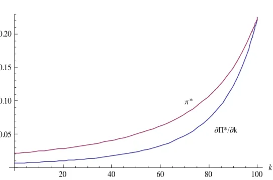
(13) 0.20. 0.15. p*. 0.10. ∑P*/∑k. 0.05. 20. 40. 60. 80. 100. k. Figure 1: Marginal profits from holding an extra supplier. while the second term represents the indirect (or strategic) effect on Π which comes from the induced rise in the equilibrium negotiated price of inputs supplied by the remaining independent suppliers. The fact that the marginal profit of owning one more subsidiary is lower than the equilibrium profit of an independent upstream entity provides an intuitive explanation of the tendency for vertical disintegration in the Markov equilibrium of the dynamic game which we investigate below. Figure 1 shows the relationship between Π ( ) and ( ) for  = 100  =??? and  =????. (Please delete the asterisk * in Figure 1, at two places.). 3. Optimal disintegration when the downstream firm can commit. In this section we suppose that the downstream firm can commit to a time path () which is achieved by a program of selling some subsidiaries or buying some independent upstream entities at the market price, denoted by 10.

(14)  (). (Note that the total number of upstream entities is always fixed at .) We suppose that the asset price  () is “correct” in the sense that it is equal to the discounted stream of (expected) future profits of an independent upstream supplier:13  () =. Z. ∞. −(−) (() ). (8). . where (() ) is given by (1). The downstream firm therefore completely determines  () by committing to a path of (). From (8), the evolution of asset price is given by ˙ () =  () − (() ) This condition is the usual non-arbitrage condition in a competitive asset market: the return to holding an asset (namely, the sum of capital gain, ˙  and dividend, ) is just equal to the opportunity cost,  , of forgone interest income. In what follows, we will treat () as a real number, where  ∈ [0 ], and ˙ interpret () as the rate at which the downstream firm acquires (or sells, if ˙ is negative) upstream subsidiaries. The downstream firm  (or, more precisely, the partially integrated firm), ˙ to maximize knowing that  () is determined by (8), chooses a time path () the present value of the stream of its net receipts: Z ∞ h i − ˙  (0 ) = max  Π(() ) −  ()()  ˙. 0. subject to (0) = 0 (given), and () ∈ [0 ]. Write. −. () ≡ . −.  () = . Z. ∞. −(−) (() ). . 13. Thus, if the downstream firm  commits to a time path ∗ (), it is implicitly telling the market that the asset price at time  is Z ∞ ∗  () = −(−) (∗ () ) . 11.

(15) Since  is bounded, it is clear that lim→∞ () = 0. Then, upon integration by parts, Z Z ∞ − ˙   ()() = 0. ∞. 0. −(0). Z. ∞. Z ˙ ()() = [(∞)(∞) − (0)(0)]−. −. . ∞. ˙ ()() =. 0. (() ) +. 0. Z. ∞. ()− (() ). 0. Thus the objective function of  becomes Z ∞  (0 ) = max − [Π(() ) − (() − 0 )(() )]  s.t. () ∈ [0 ] . 0. (9). Since the objective function (9) contains only the variable , the solution of this optimization problem can be described succinctly as follows. For any 0  , it is optimal to make an immediate jump in the state variable (an impulse control) to some level (0+ ) = , and after this initial jump, () will be kept constant at  for ever, where  is the value of  that maximizes (; 0  ) ≡ (Π( )) − ( − 0 )(( )) subject to  ∈ [0 ]. That. is, the firm chooses its immediate net acquision,  − 0  of subsidiaries to. maximize the present value of the profit flow, Π, minus the cost of acquision (i.e., the price of (( )) per unit, multiplied by the number of units acquired,  − 0 ). Note that in principle  − 0 can be positive (acquision). or negative (sale of some subsidiaries).. Using the definition of  and the property (6), we obtain the derivative ¶ µ −   (; 0  ) = Π −−(−0 ) = −   −(−0 )  = (20 −  − ) 2 2 (10) Since    0, we see that  has the sign of (20 −  − ). It follows that. the function (; 0  ) is (i) strictly decreasing in  for all  ∈ (0 ] if. 0 ≤ 2, (ii) strictly increasing in  for all  ∈ (0 ) if 0 = , and (iii) ¡ ¢ hump-shaped in  if 0 ∈ 2   . The value  that maximizes (; 0  ). must satisfy the following first order condition:. Π ( ) − [( ) + ( − 0 )  ( )] ≤ 0 ( = 0 if   0) 12.

(16) The following re-arrangement facilitates the interpretation of the first order condition: 1 1 1 Π ( ) ≤ ( ) − (0 − )  ( ) (with equality if   0).    The term 1 ( ) − 1 (0 − )  ( ) is the marginal revenue from reducing.  (i.e. from selling an extra subsidiary), while the term. 1 Π ( )  . is the. marginal loss of income flows from operating a smaller integrated firm. At , the two terms are equated, unless it is a corner solution. Using (10) the first order condition reduces to 20 −  −  ≤ 0 This condition gives the following rule that determines the optimal number of subsidiaries to keep after an initial sale of assets:14  = min {20 −  0}. (11). The rule (11) allows us to state our first proposition: Proposition 1 (Optimal asset sale strategy under commitment). If the downstream firm can make binding commitment on its time path of asset holding, its optimal policy is as follows. Case (i): 0 = . In this case,  = , i.e., it is optimal not to sell any subsidiary if firm  initially owns all the  upstream entities. £ ¤ Case (ii): 0 ∈ 0 2 (i.e., firm  initially does not own more that half. of the number of upstream entities). In this case, firm ’s optimal action is. to sell immediately all its subsidiaries, i.e.,  = 0. ¡ ¢ Case (iii): 0 ∈ 2   (i.e., the number of independent upstream suppliers, while positive, is smaller than half of the input suppliers). In this case, it is optimal for the firm to sell some, but not all, of its upstream assets, causing  to jump down from 0 to a strictly positive level  = 20 −   0. The second order condition is satisfied, because 1 Π( ) + 1 (0 − )( ) is strictly quasi-concave in . 14. 13.

(17) Remark 3.1: In cases (ii) and (iii), the price at which a subsidiary would be sold is. 1  (0) = ( )  This follows from (8). Given that  is able to commit to keeping  for ever. after the initial sale, the market expects that the present value of the stream of revenue generated by an independent upstream entity is ( ). Remark 3.2: If the downstream firm can commit to the open-loop strategy described in Proposition 1, the value of its program is ½ ¾ 1 ( )  (0 ) = Π( ) + (0 − )   where the term inside {} represents the proceeds from the immediate sale. of (0 − ) subsidiaries.. Remark 3.3: The solution described in Proposition 1 displays the property of time-inconsistency in case (iii). In this case the open-loop strategy of holding () = 20 −   0 for all  ∈ (0 ∞) implies that at any time. 1  0, if firm  would be released from its original commitment, it would again want to sell immediately some more subsidiaries, and a price below the initial price ( ). This action would inflict capital losses to the previous buyers of subsidiaries, because they have been fooled into believing that the downstream firm would sell assets only once. Solutions that display timeinconsistency are generally regarded as unacceptable (Coase, 1972). Therefore we must look for time-consistent solutions.. 4. Markov-perfect equilibrium. In this section, we seek solutions that have the time-consistent property, and, in addition, that would be robust to perturbation. More precisely, we are insisting on a stronger property than time-consistency, namely Markov perfect. 14.

(18) equilibrium.15 In a Markov perfect equilibrium, firm  uses a Markovian strategy  and the market has a Markovian price function, or expectation rule,  (which we will explain in more detail below) such that (i) given , the Markovian strategy  maximizes firm ’s payoffs, for all possible starting (state, date) pairs (  ), and (ii) given , the Markovian price function  is consistent with rational expectations.16 We assume that all investors (potential buyers of assets) have a common Markovian asset price expectation rule  = (), i.e., the asset price expected to prevail at any time  is a function of the concurrent level () of the state variable. The function () maps [0 ] into the set of positive real numbers, and we permit  to be piece-wise continuous in . A Markovian expectation rule  is said to be rational if ( ) = . Z. ∞. −(−) (() ). (12). . where  is the expectation operator, and {()}∞  denotes the time path of. the state variable induced by the use of the Markovian strategy  from time  when the state variable takes the value  . We now seek to describe plausible Markovian strategies for firm . We know that if 0 = , the firm is a fully integrated monopoly, so there is no gain in selling assets. We restrict attention to the set of initial conditions 0 ∈ [0 ). We suppose that a strategy  specifies some positive real number.  ≤  with which the set [0 ) is partitioned into three disjoint subsets, [0 ), {}, and ( )  where the set {} is a singleton.. We will show that if the initial condition  is in the set [0 ), then the. firm will make a lumpy sale  = () which causes a jump in the state variable, with jump size  ∈ [ −  ] i.e., if (0) = 0 then (0+ ) = 0 − . Note that  can in principle be positive or negative; a positive (negative)  15. For an exposition of the concepts of time-consistency and Markov perfect equilibrium, and a proof that Markov perfect equilibria are time-consistent, see Dockner et al. (2000). Long (2010) provides some simple examples. 16 For some examples of Markovian price function in the industrial organization literature, see Driskill and McCafferty (2001), and Laussel et al. (2004).. 15.

(19) means a downward (upward) jump, i.e. a lumpy sale (purchase) of assets. The function  (), defined over [0 ), is specified by the strategy . We will also show that if the initial condition is in the set ( ), then the firmwill apply a gradual purchase/sale policy () such that ˙ = () where  is a bounded function, i.e., there is no jump in the state variable when  ∈ ( ). If ()  0 (respectively,  0) we says the firm engages in gradual. purchase (resp., gradual sale). The function , defined over ( ), is specified by the strategy . The point  is called the “junction point.” If the initial condition is at a junction point, i.e. if  = , we allow the firm to use a mixed sub-strategy: to make a lumpy sale of size  with probability  and to stay put (i.e. neither buy nor sell) with probability 1 − . (The real numbers  and  are specified by the strategy .). Thus, a strategy  is a tuple (    ). Given the market expectation function , firm  chooses a strategy  to maximize its expected payoffs for any starting point (  ) : Z ∞ h i ˙ )  ( ) =  −( −) Π(( ) ) − (( ))( . where ˙ ) = (( )) if ( ) ∈ ( ) ( ( + ) = ( ) − (( )) if ( ) ∈ [0 )  ( + ) = (1 − )( ) +  [( ) − ] if ( ) =  We define a Markov-perfect equilibrium as a couple (∗  ∗ ) such that (i) given the market expectation rule ∗ , the strategy ∗. ≡. (∗  ∗  ∗  ∗   ∗ ) maximizes firm ’s expected payoff for any starting point (  ) (ii) given the strategy ∗ , the market expectations are rational. We now characterize Markov-perfect equilibria. We begin with a few observations.. 16.

(20) £ ¤ Obviously, if the initial 0 lies within the range 0 2 , the Markov perfect. equilibrium would dictate firm  to sell all of its upstream subsidiaries. This is because the commitment equilibrium, which would dictate the same action, £ ¤ is time-consistent for 0 ∈ 0 2 .17 We state this result as Lemma 1. £ ¤ Lemma 1: If  ∈ 0 2 then the equilibrium Markovian strategy dictates. the sale of all subsidiaries immediately. The equilibrium market expectation function satisfies. h i 1 () = (0 ) for all  ∈ 0   2 £ ¤ Proof: Selling off all subsidiaries when  ∈ 0 2 is also the solution. of firm ’s optimization problem when commitment is possible, and it is. time-consistent because after the sale,  has no more upstream assets to offer to the market. Therefore buyers will not be caught by surprise later in the game. It follows that the equilibrium is Markovian with the expectation £ ¤ function  such that () = 1 (0 ) for all  ∈ 0 2 ¥. ¡ ¢ What happens if  ∈ 2   ? Recall that if commitment were possible, ¡ ¢ then for any 0 ∈ 2   , firm  would commit to the immediate, once-only. sale of only a fraction of its subsidiaries, and keep  subsidiaries for ever, and the asset price would be 1  = ( ) . and would remain the same ever after. However, if commitment is not possible, no one is willing to buy a subsidiary at the price 1 ( ), because everyone expects that firm  will renege from its initial announcement, and will sell some more subsidiaries in the immediate future, inflicting a capital loss to the early buyers. This outcome would be inconsistent with rational ¡ ¢ expectations. The question is then, if 0 ∈ 2   would the Markov per-. fect equilibrium requires firm  to sell off all subsidiaries immediately? If 17. The commitment equilibrium is time-consistent in this range because after the immediate sale at time 0+ , firm  has no more subsidiaries to sell.. 17.

(21) not, what is the upper bound on 0 such that the policy of selling off all subsidiaries immediately is better than keeping all of them for ever? Selling all 0 immediately would give  the sale revenue of 0 (0 ). In addition to this, firm  would also earn a stream of profit Π(0 ) per unit of time after the sale of all its subsidiaries. The sum of these two sources of revenue is, in present value terms, 1 1 (0 ) ≡ 0 (0 ) + Π(0 )   Consider an alternative policy, that of keeping 0 for ever. The capitalised value of the resulting income stream would be 1 Π(0  ). Lemma 2: The set of 0 such h ithat (0 ) is greater than or equal to is the closed interval 0 e  where e  is the threshold level defined. 1 Π(0  ) . by. where. 1 e ≡ [3(2 − ) + 4 − ]   4 ≡. p 9(2 − )2 + 8(2 − ). (13). (14). Proof: Observe that 1 Π( ) is a strictly convex function of  in [0 ], and () is linear in , with (0) − 1 Π(0 ) = 0, and 0 (0) − 1 Π (0 )  0.. Therefore the function ()− 1 Π( ) is strictly concave and its value is equal to zero at exactly two points,  = 0 and  = e , where e    is the unique positive root of the following equation18 1 Φ() ≡ [Π(0 ) + (0 ) − Π( )] = 0  This yields i p 1 h e = 3(2 − ) + 4 − 9(2 − )2 + 8(2 − )  0¥ 4. (15). Remark 4.1: Lemma 2 implies that e  is the threshold number of subsi-. diaries below which firm  would prefer selling them all at once to keeping 18. The condition Φ() = 0 yields a cubic equation, of which one of the roots is zero. The other two roots are real and of opposite signs. We select to positive root e . Laussel (2008) e shows that  is bounded below by 23 (it tends to 23 as  → 0, and it is increasing in ), and e  is strictly smaller than 1 for all finite .. 18.

(22) them all for ever.19 Thus, we can conclude that if 0  e , it is not optimal to sell off all subsidiaries immediately. Obviously, e  is a logical candidate for ∗ ∗ ∗ ∗ ∗ ∗ ∗ when we fully characterize the strategy ³ ´ ≡ (         ). Can we conclude that for 0 ∈   e   the policy of selling off all subsidi2. aries is better for  than any policy of gradual sale that meets the rational. expectations requirement? The answer is provided in Lemma 3 below. ³ ´ Lemma 3: If 0 ∈ 2  e  then, facing a Markovian market expectation function (), to sell assets gradually cannot be an equilibrium strategy. ³ ´  e Proof: Assume that 0 ∈ 2   .The policy of selling all subsidiaries. immediately gives firm  the payoff 1 Π(0 ) + 0 (0 ). Suppose the. firm considers an alternative strategy, say  , of selling its upstream entities gradually until some level b  (where 0 ≤ b   0 ≤ e ) is reached, at which point it will sell all of b . We will show that this alternative policy violates the necessary conditions of firm ’s optimal behavior, given the rational expectations requirement.The policy  would give the payoff Z  h i − ˙ Π(  ) − ( )  + − (b  ) 0. where. (0 ) 1 (b ) ≡ b  + Π(0 )   Z ∞ ( ) = −(−) (() ). and. (16). . Consider the following problem with free time  and a fixed endpoint , where   e  Z  h i ˙  + − (b max − Π(() ) − (())() ) ˙ . 0. subject to (0) = 0 and ( ) = b . Let  denote the co-state variable. The. Hamiltonian function is.  = Π( ) − ()˙ + ˙. As shown in Laussel (2008), for all   0, the ratio e  is increasing in  and tends to 1 as  tends to infinity. 19. 19.

(23) If selling assets gradually is an equilibrium, then the following conditions must hold.  = −(()) + () = 0 for all  ∈ [0  ]  ˙. (17).  0 ˙ ˙ (()) for all  ∈ [0  ] = () − Π (() ) + () () = () − () (18) and the transversality condition is20  h − b i − ( ) − )  () = 0, i.e. ( ) = (b . (19). Differentiating equation (17) gives. 0 ˙ ˙ (()) () = (). (20). () = Π (() ). (21). From (18) and (19),. From (17) and (21), we deduce that if gradual sale is an equilibrium, then it must holds that () =. Π ( ) . (22). and thus. Π ( )  Now, differentiating the market expectation rule (16), we get 0 () =. 0 ()˙ = () − ( ). (23). (24). Using (24) and (23), we get Π − ( )  − ( ) = 0 ˙ = 1 0  () Π   i.e. ˙ = − 20.  ( − ) [( −  − 1) + 2]  0 3(2 − ). See, e.g., Leonard and Long (1992, Chapter 7).. 20. (25). (26).

(24) With the use of (17), the transversality condition (19) reduces to 1 (b ) = Π(b  ) . i.e.. (0 ) 1 1 b  + Π(0 ) = Π(b  )    b e b b e This equation³implies ´ that either  =  or  = 0. But  =  is not possible, because 0 ∈ 2  e  and ˙  0 by (25). Consider the possibility that b  = 0.. Then equation (26) together with the boundary conditions (0) = 0 and ( ) = b  = 0 yields the solution path21 () =  − h. 1 −0. +.  2−. i. 1. −3 −. ¡.  2−. ¢ for  ∈ [0  ]. where  is determined by the condition ( ) = 0, i.e., 3  = ln . ". 1  + 2− −0 1  + 2− . #. This implies that, according to the Markovian market expectation rule (), the asset price at  is expected to be, by (22), 1 (2 − )2  ( ) = (( )) = Π (0 ) =  2 [(2 − ) + ]3 However, the present value of the income stream generated by an asset from time  onwards is Z ∞ 1 (2 − ) 1 +  ( ) = −(− ) (0 ) = (0 ) =   ( )  2 [(2 − ) + ]2  This upward jump in asset price is inconsistent with rational expectations. It follows that b  = 0 is not admissible either. ³ ´ This completes the proof that the policy of gradual sale when 0 ∈ 2  e  is not consistent with equilibrium.¥ 21. See Appendix.. 21.

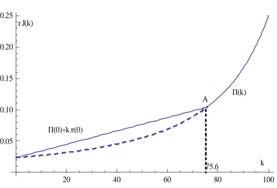
(25) It remains to find the equilibrium strategy ³ ´ for other initial conditions, namely, (i) for 0 = e , and (ii) for 0 ∈ e   . ³ ´   the equilibrium policy is to sell the assets We will show that if 0 ∈ e . gradually, until  reaches the value e Lemma 4:. : (i) For 0 = e At  = e , firm  sells all of its subsidiaries with probability  and keeps. all its subsidiaries with probability 1−, where  is specified below. While firm  is indifferent about the value of , the requirement that market expecation ∗ be rational implies that in equilibrium  must be the solution of . ´ (0 ) (e  ) 1 ³ + (1 − ) = Π e     . (27). i.e. the expected value of the dividend flow of an independent upstream entity (the left-hand side of equation (27)) is equal to the value of the market e 22 expectation function ³ () ´ evaluated at . (ii) For 0 ∈ e   : ³ ´ If 0 ∈ e   then in equilibrium firm  sells its assets gradually until  reaches the value e . The equilibrium gradual purchase/sale policy is. ³ ´  Π ( ) − ( ) e =− (−) [( −  − 1) + 2]  0 for all  ∈   . () = 1 3(2 − ) Π ( )   (iii) The equilibrium market expectation function () is piece-wise con-. tinuous in , and satisfies the property that ³ ´ 1 1   () = Π ( )  ( ) for  ∈ e   ´ ³ ´ 1 ³   for  = e , where (0 )  Π e    ( ) (e ) = Π e . 22. Solving for , one gets =. where  is given by (14).. 16 [ − 3(2 − )] h i 0 16 1 (2 −  + )3 (2−+) 2 − (2−+)2. 22. (28) (29).

(26) and. ³ ´ 1 () = (0 ) for  ∈ 0 e  (30)  Remark 4.2: From equations (28), (29) and (30), () is piece-wise dis-. continuous in , with lim ()  (e ) = lim (). ↑ . ↓ . Investors who purchase the asset when   e  do not make losses when  ↓ e , because the non-arbitrage condition (12) holds for them.. Proof of lemma 4: Since the right-hand side of (15) is equal to zero when evaluated at e , we know that when 0 = e , firm  is indifferent between (a) keeping e  subsidiaries for ever, and (b) selling them all immediately. Either. action will yield the same payoff to firm , ³ ´ 1 1  e  = Π(e  ) = e  (0 ) + Π(0 ) (31)   However, if firm  were to choose action (a) with probability 1, the market would expect the asset price to be Z ∞ 1 1  )  Π (e 1 ≡ − (e  ) = (e  )   0. (32). thus the market would expect that the asset price to be Z ∞ 1 1 2 ≡ − (0 ) = (0 )  Π (e  )   0. (33). while if  were to choose action (b) with probability 1, then (0+ ) = 0, and. If  randomizes its choice of action at e  using probability  for (b) and. 1 −  for (a), the market expectation is. (e ) = (1 − )1 + 2. (34). We will determine  toward the end of this proof.. ³ ´ Let us determine the gradual purchase/sale policy for  ∈ e   . Given ³ ´ 0 ∈ e   , firm  solves the following fixed endpoint problem:  (0 ) = max ˙ . Z. 0. . −. . h i ˙ ) Π(() ) − (())()  + − (e 23. (35).

(27) where (e ) is given by (31), subject to (0) = 0 and ( ) = e  (fixed). The solution to problem (35) can be found by using either the maximum principle, or the dynamic programming approach.. (A) solution using the maximum principle Let  denote the current-value Hamiltonian and  denote the currentvalue shadow price. Then ˙ + ()() ˙  = Π(() ) − (())() Then, using an argument similar to that used in the proof of Lemma 3, we deduce that ˙ = −.  ( − ) [( −  − 1) + 2]  0 3(2 − ). At time  , it is required that ( ) = e . Therefore  3. . =. This equation determines  :. 1  + 2− −0 1  + 2− − . 3  = ln . ".  1 for 0  e . 1  + 2− −0 1  + 2− − . #. . (36). (B) solution using Hamilton-Jacobi-Bellman (HJB) equation We will show that the value function is ½ ¾ 1 1 1 () = max Π( ) Π(0 ) +  (0 )    i.e. () =. (. 1 Π(0 ) +  1 Π( ) .  1 (0 ) if 0 ≤  ≤ e  . e if  ≤  ≤ . ³ ´ Over the interval e   we have the HJB equation. h i ³ ´ ˙ ˙ e () = max Π( ) − () +  () for  ∈   ˙. 24. (37). (38). (39).

(28) For a finite ˙ to be optimal, it is necessary that ³ ´   () =  for  ∈ e. (40). Substitute this into (39) to get. ³ ´ e () = Π( ) for  ∈  . (41). which confirms (38). Differentiate (41),. ³ ´ 1    () = Π ( ) for  ∈ e . (42). Substituting (42) into (40) we obtain the market expectation function ³ ´ 1 () = Π ( ) for  ∈ e   . (43). Since assets are sold gradually, investors would purchase while   e  if. and only if. i.e.,. lim () = (e ) ↓ . 1 (e ) = Π (e  ) . (44). where (e ) denotes the expected asset price at  = e . Condition (44) is necessary to suuport the equilibrium, because if (e )  1 Π (e  ) then no one would want to buy assets when  is greater than e  (they would be making. capital losses when  reaches e ). And if (e )  1 Π (e  ), everyone would. make capital gains by delaying purchases until  is just infinitessimally above e  For   e , we use (38) to obtain the market expectation function 1 () = (0 ) . (45). While equations (43) and (45) indicates that the market expectation function is discontinuous in , we can see that in equilibrium, the path of expected asset price  () is continuous, i.e.  is a continuous function of time. From 25.

(29) 0.25 r J(k) 0.20. 0.15 P(k). A 0.10 P(0)+k p(0). 0.05 75.6 20. 40. 60. 80. k 100. Figure 2: Equilibrium value of the assembler’s problem as a function of  ³ ´ any  ∈ e   , the asset price will be falling continuously, until  reaches e  ) with probability , at which point the asset price will jump up to 1 (e . 1 −  and jump down to. 1 (0 ) . with probability .¥. Remark: Equation ³ ´ (38) shows that, in a game where  can buy or sell   , its Markov-perfect equilibrium payoff is just equal to assets, if 0 ∈ e. what it would earn in the alternative scenario where it were not allowed to ³ ´ e engage in buying and selling assets. In contrast, if 0 ∈ 0  , its Markovperfect equilibrium payoff is higher than what it would earn in the alternative. scenario.. We can now state our main proposition. Proposition 2: The Markov-perfect equilibrium of the asset purchase/sale game is as follows. 1. Firm  sells immediately all its downstream subsidiaries if   e .. 2. If  = , ³ firm ´  keeps all its subsidiaries for ever. 3. If  ∈ e   , firm  gradually sells its subsidiaries according to the 26.

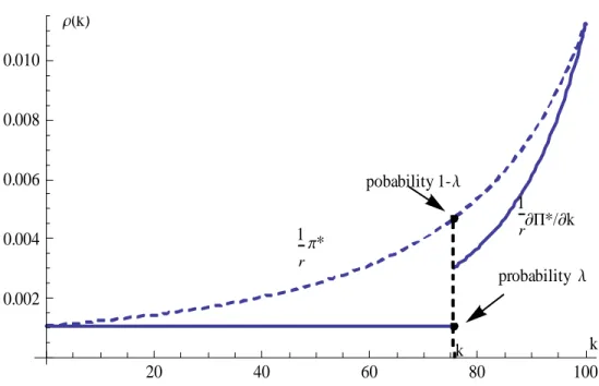
(30) r(k). 0.010 0.008 pobability 1- l. 0.006. 1 ∑P*/∑k r. 1 p*. 0.004. r. probability l. 0.002 k. k 20. 40. 60. 80. 100. Figure 3: The equilibrium buyers’ price strategy selling rule −() =. ( ) − Π ( ) 0 1 Π ( )  . This will continue until e  is reached in finite time. 4.If  = e , firm  will sells all e  immediately with probability , and keep all e  for ever with probability 1 −  5. The market has the following Markovian asset price expectations func-. tion. () =. ⎧ ⎪ ⎪ ⎨ ⎪ ⎪ ⎩. 1 Π ( )   1 Π (e  )   1 (0 ) . ³ ´ if  ∈ e   if  h= e ´ . if  ∈ 0 e . ³ ´  , the downstream firm’s equilibrium payoff is strictly greater If 0 ∈ 0 e. than what it would earn in the alternative scenario where it were not allowed to buy or sell asset.. 27.

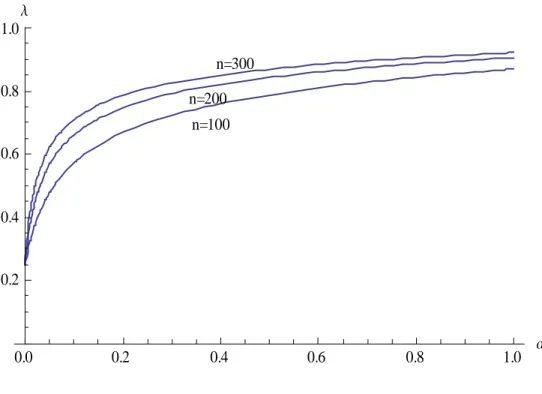
(31) l. 1.0 n=300 0.8. n=200 n=100. 0.6. 0.4. 0.2. 0.0. 5. 0.2. 0.4. 0.6. 0.8. 1.0. a. Figure 4: The probability of selling all subsidiaries at  = e .. Concluding Remarks. We have shown that the dynamics of vertical disintegration imply either a very quick (in fact instantaneous) convergence toward a fully disintegrated structure, when the initial number of upstream subsidiaries is small, or a very slow process of separation which may take many years, when when the initial number of upstream subsidiaries is large. The model yields the prediction that one should observe either very disintegrated vertical structures or very integrated ones slowly evolving through progressive outsourcing. It also predicts that it is more likely to reach a final stage of full disintegration when the upstream firms’ bargaining power is great. These predictions are consistent with empirical evidence: first, as stated in the introduction, there is a tendency to vertical separation; second, the Japanese auto industry, where the component suppliers have a greater bargaining power, is much more disintegrated than its US counterpart. Of course, the instantaneous disintegration result, in the case where the initial number of subsidiaries is lower than the 28.

(32) critical value, appears somewhat brutal. But this outcome would have been mitigated, had we introduced some adjustment costs. This is a possible extension of this paper. Another direction of generalization would be to consider several competing downstream firms. In the latter case, at least if donstream firms compete in prices, we conjecture that this would reinforce the tendency toward outsourcing which would be, in addition to being a defense against strong suppliers, a way to soften downstream competition.. Appendix A.1. Proof : solution of the main differential equation. Define  ≡− Then equation (26) becomes ∙ ¸   ˙ =  +1 3 2− 0r. ³´ µ  ¶  ˙ −  = 2 3 3 2−. Multiply both sides by  −2. µ ¶   −1 ³  ´  ˙ −  = 3 3 2− −2. Define.  =  −1 ⇐⇒ ˙ = − −2 ˙ Thus. or. Then. ³´ µ  ¶  −˙ −  = 3 3 2−. ³´ µ  ¶  ˙ +  = − 3 3 2−. ³´ µ  ¶ h  i 3 =− 3 ˙ +   3 3 2− 29.

(33) Integrating. Then. Z h ³ ´ µ  ¶ Z   i  3 ( ˙ ) +    = −  3  3 3 2− 0 0 µ. ¶ ¤ £ 3  () − 0 = − −1  2− µ ¶ ¤ £ 3 1 3 1  − =− −1    0 2− ∙ ¸ µ ¶ 1 3 1   = +  − 3  0 2 −  2− µ ∙ ¸ ¶ 1   1 −3 + − =   0 2 −  2− 1 i  =− = h ¡  ¢ 1  −3 − 2− + 2− 0 3.  =− h. () =  − h. 1 0. +. 1 −0.  2−. +. i. 1. −3 −.  2−. i. 1. ¡.  2−. −3 −. ¡. ¢.  2−. ¢. Suppose we impose the boundary value ( ) = b  for some b  ≥ 0. Then ∙. h. 1 −0. +.  2−. i. 1. − 3. −. ¡.  2−.  ¢ =−b. ¸ ¶ µ 1 1   − 3  = + −  − 0 2 −  2− −b  ¸ ∙ 1  1  − 3 = + +  − 0 2 −  −b  2−  3 =. This equation determines  .. 1  + 2− −0 1  + 2− − . 3  = ln . ".  1 for 0  b . 1  + 2− −0 1  + 2− − . 30. #.

(34) References [1] Amir,R., 1996, Continuous stochastic games of capital accumulation with convex transitions, Games and Economic Behavior, 16, 111-131. [2] Ausubel, L. and R. Deneckere, 1989, Reputation and Bargaining in Durable Goods Monopoly, Econometrica 57(3), 511-532. [3] Bonanno, G. and J. Vickers, 1988, “Vertical Separation,” Journal of Industrial Economics 36, 257-265. [4] Bond, E. and L. Samuelson, 1984, Durable Goods Monopoly with Rational Expectations and Replacement Sales, Rand Journal of Economics 15, 336-345. [5] Bond, E. and L. Samuelson, 1987, The Coase Conjecture Need not Hold for Durable Good Monopolies with Depreciation, Economics Letters 24, 336-345. [6] Chen, Y., 2001, “On Vertical Mergers and Their Competitive Effects,” RAND Journal of Economics 32, 667-685. [7] Chen, Y., 2005, “Vertical Disintegration,”Journal of Economics and Management Strategy, 14, 209-229. [8] Coase, R., 1972, Durability and Monopoly, Journal of Law and Economics, 15, 143-9. [9] Corswant, Fredrick von, and Peter Fredriksson, 2002, “Sourcing Trends in the Car Industry, A Survey of Car Manufacturers’ and Suppliers’ Strategies and Relations,” International Journal of Operations & Production Management, 22(7), 741 - 758. [10] Cournot, A.A., 1838, Recherches sur les Principes Mathématiques de la Théorie des Richesses, Paris: Hachette.. 31.

(35) [11] Cusumano, M., and A. Takeishi, A., 1991, “Supplier Relation and Management: A Survey of Japanese, Japanese-transplant, and U.S. Auto Plants,” Strategic Management Journal, Vol. 12, 563-88. [12] DeMarzo, Peter M., and Branko Urošević, 2006, “Ownership Dynamics and Asset Pricing with a Large Shareholder,” Journal of Political Economy 114(4), 774-814. [13] Dockner, E., S. Jørgensen, N.V. Long, and G. Sorger (2000), Differential Games in Economics and Management Science, Cambridge University Press, Cambridge, U.K. [14] Driskill, Robert, 1997, “Durable-Goods Monopoly, Increasing Marginal Cost, and Depreciation,” Economica 64(253), 137-54. [15] Driskill, R. and S. McCafferty (2001), “Monopoly and Oligopoly Provision of Addictive Goods,” International Economic Review 42(1): 43-72. [16] Economides, N. and S.C. Salop, 1992, “Competition and Integration Among Complements, and Network Market Structure,” Journal of Industrial Economics, 40, 105—123. [17] Gal-Or, E. 1999, “Vertical Integration or Separation of the Sales Function as Implied by Competitive Forces,” International Journal of Industrial Organization 17, 641-662. [18] Gaudet, G. and S. Salant, 1992a, Mergers of Perfect Complements Competing in Price, Economics Letters, 39, 359—364. [19] ––and––, 1992b, “Towards a theory of horizontal mergers,” in G. Norman and M. La Manna, eds., The New Industrial Economics: Recent Developments in Industrial Organization, Oligopoly and Game Theory, London: Edward Elgar. [20] ––and N. V. Long, 1996, “Vertical Integration, Foreclosure and Profits in the Presence of Double Marginalization,” Journal of Economics and Management Strategy, 5, 409—432. 32.

(36) [21] ––, N. V. Long, and A. Soubeyran (1999) “Upstream-Downstream Specialization by Integrated Firms in a Partially Integrated Industry,” Review of Industrial Organization, 14, 1999, 321-335 [22] Gomes, Armando, 2000, “Going Public eithout Governance Managerial Reputation Effects,” Journal of Finance, Vol. 55(2), 615-645. [23] Greenhut, M.L. and H. Ohta, 1979, “Vertical Integration of Successive Oligopolists,” American Economic Review, 69, 137—141. [24] Gul, F., H. Sonnenschein and R. Wilson, 1986, “Foundations of Dynamic Monopoly and the Coase Conjecture, Journal of Economic Theory 39, 155-90. [25] Kahn, C. 1987, “The Durable Goods Monopolist and Consistency with Increasing Costs,” Econometrica 54, 274-294. [26] Kamien, M.I. and I. Zang, 1990, “The Limits of Monopolization Through Acquisition,” Quarterly Journal of Economics, 105, 465—500. [27] Karp, L., 1996a, “Monopoly Power can be Disadvantageous in the Extrcation of a Durable Nonrenewable Resource,” International Economic Review 37(4), 825-49. [28] Karp, L., 1996b, “Depreciation Erodes the Coase Conjecture,” European Economic Review, 40, 473-490. [29] Laussel, D., 2008, “Buying Back Subscontractors: The Strategic Limits of Backward Integration,” Journal of Economics and Management Strategy, 17, 895-911. [30] Laussel, D., M. de Montmarin, and N. V. Long (2004), “Dynamic Duopoly with Congestion Effects,” International Journal of Industrial Organization 22 (5), 655-677.. 33.

(37) [31] Léonard, D. and N.V. Long, 1992, Optimal Control Theory and Static Maximization in Economics, Cambridge University Press, Cambridge, U.K. [32] Lin, P., 2006, Strategic Spin-Offs of Input Divisions,” European Economic Review 50, 977-993. [33] Maskin, E and J. Tirole, 2000, “Markov Perfect Equilibrium I: Observable Actions,” Journal of Economic Theory 100: 191-219. [34] Matsushima, Noriaki and Tomomichi Mizuno, 2009, "Vertical Separation as a Defense against Strong Suppliers," Institute of Social and Economic Research Discussion Paper n◦ 755, Osaka University. [35] Matsushima, Noriaki and Tomomichi Mizuno, 2009,“ How Do Market Structures Affect Decisions on Vertical Integration/Separation?” Institute of Social and Economic Research Discussion Paper n◦ 770, Osaka University. [36] Milliou, C. and E. Petrakis, 2007, “Upstream Horizontal Mergers, Vertical Contracts and Bargaining,” International Journal of Industrial Organization, 25, 963—987. [37] Perry, M.K., 1989, “Vertical Integration; Determinants and Effects,” in R. Schmalensee and R. D. Willig, eds., Handbook of Industrial Organization, New York: North Holland,183—255. [38] Salant, S. W., S. Switzer, and R. J. Reynolds, 1983, “Losses from Horizontal Merger: The Effects of an Exogenous Change in Industry Structure on Cournot—Nash Equilibrium,” Quarterly Journal of Economics, 98, 185—199. [39] Shy, O. and R. Stenbacka, 2003, "Strategic Outsourcing," Journal of Economic Behavior and Organization, 50, 203-224.. 34.

(38) [40] Sonnenschein, H., 1968, “The Dual of Duopoly is Complementary Monopoly, or Two of Cournot’s Theories are One,” Journal of Political Economy, 76, 316—318. [41] Stokey, N. 1981, “Rational Expectations and Durable Goods Pricing,” Bell Journal of Economics 12, 112-128.. 35.

(39)