Morphing Wing: Experimental Boundary Layer Transition
Determination and Wing Vibrations Measurements
and Analysis
by
Yvan Wilfried TONDJI CHENDJOU
THESIS
PRESENTED TO ÉCOLE DE TECHNOLOGIE SUPÉRIEURE IN PARTIAL
FULFILLEMENT FOR A MASTER'S DEGREE WITH THESIS IN
AEROSPACE ENGINEERING
M.A.Sc.
MONTREAL, 12TH DECEMBER 2016
ÉCOLE DE TECHNOLOGIE SUPÉRIEURE UNIVERSITÉ DU QUÉBEC
© Copyright reserved
It is forbidden to reproduce, save or share the content of this document either in whole or in parts. The reader who wishes to print or save this document on any media must first get the permission of the author.
BOARD OF EXAMINERS
THIS THESIS HAS BEEN EVALUATED BY THE FOLLOWING BOARD OF EXAMINERS
Ms. Ruxandra Botez , Thesis Supervisor
Department of Automated Manufacturing Engineering at École de technologie supérieure
Mr. Christian Belleau, President of the Board of Examiners
Department of Mechanical engineering at École de technologie supérieure
Mr. Tony Wong, Member of the jury
Department of Automated Manufacturing Engineering at École de technologie supérieure
THIS THESIS WAS PRENSENTED AND DEFENDED
IN THE PRESENCE OF A BOARD OF EXAMINERS AND PUBLIC ON NOVEMBER 28, 2016
ACKNOWLEDGMENT
I would like to thank my research supervisor Professor Ruxandra Botez for her support and for the opportunity to improve my technical skills through this master thesis. I also wish to thank Dr Lucian Gregorie and Mr. Oscar Carranza Moyao, research associates at the LARCASE, for their invaluable advice.
Secondly, I would like to thank Mr. Vincent Ruault, for his technical assistance and precious advice during the realization of my thesis at the LARCASE.
I would also like to offer my appreciation to the project's partners: Thales Canada, Bombardier Aerospace, École Polytechnique de Montreal, IAR-NRC, CIRA, Alenia Aeronautica and Naples Frederico University II for their technical and financial support.
Many thanks are due to all the past and present LARCASE members who participated and contributed to the realization of this project, especially to Dr Joel Tchatcheng, Dr Andreea Koreanschi, Dr Oliviu Sugar-Gabor, and Mr Manuel Flores Salinas.
Finally, I wish to express my sincere thanks to my family for supporting me morally and financially throughout my Master's studies.
AILE ADAPTABLE: DETERMINATION EXPERIMENTALE DE LA ZONE DE TRANSITION DE LA COUCHE LIMITE, MESURE ET ANALYSE DES
VIBRATIONS DE L'AILE Yvan Wilfried TONDJI CHENDJOU
RÉSUMÉ
Le présent mémoire de recherche est rédigé dans le contexte du projet international multidisciplinaire CRIAQ MDO-505 qui se déroule au Canada. Le but du projet est de concevoir, fabriquer et tester une aile déformable dont la peau flexible de son extrados peut changer de forme grâce au système d'actionnement installé à l'intérieur de l'aile. Ce changement de forme a pour but de retarder l'apparition de la zone de transition du régime laminaire au régime turbulent dans l'écoulement autour de l'aile, se traduisant ainsi par l'amélioration des performances aérodynamiques.
Cette recherche se concentre sur les différentes technologies utilisées pour acquérir les données de pressions pendant les tests en soufflerie ainsi que sur les différentes méthodologies de traitement des données de pressions dans le but de caractériser et d'analyser l'écoulement aérodynamique autour de l'aile. Ensuite, ce document présente les mesures de vibrations effectuées sur l'aile pendant les tests en soufflerie, et leur représentation graphique en temps réel. L'acquisition de ces données de vibrations est détaillée, ainsi que les méthodes de traitement de ces données qui confirment les prédictions des analyses numériques aéroélastiques.
Les données de pressions ont étés collectées en utilisant trente-deux capteurs de pression piézoélectriques capables de capter avec une très grande sensibilité des fluctuations de pression allant jusqu'à 10 KHz. Ces capteurs étaient disposés sur deux lignes de cordes et ils sont connectés à un système d'acquisition en temps réel National Instrument PXI. Les données collectées étaient par la suite filtrées, analysées et visualisées grâce aux algorithmes de la Transformée de Fourrier Rapide et aux algorithmes de moyenne quadratique; ceci était réalisé dans le but de quantifier les fluctuations de pressions présentes dans l'écoulement de l'air autour de l'aile. L'interprétation de ces fluctuations fut nécessaire pour la détection de la zone de transition du régime laminaire au régime turbulent. Environ 30% des conditions de vol testées en soufflerie ont révélé une réduction de trainée suite au changement de forme du profil d'aile. Les résultats obtenus grâce à l'analyse des données de pression ont été comparés aux résultats obtenus avec la technique de visualisation infra-rouge, et nous ont servi plus tard pour la validation des simulations numériques aérodynamiques préalablement effectuées. Deux accéléromètres analogiques capables de capter des variations d'accélérations allant jusqu'à ±16g ont étés installés dans l'aile et dans l'aileron, pour obtenir les mesures de vibrations du prototype. Les accélérations mesurées par les capteurs étaient acheminés par un
système d'acquisition NI et ont été traités en temps réel grâce à un programme LABVIEW, permettant la visualisation en temps réel, ainsi que la sauvegarde des données. Les données enregistrées ont été analysées pour prouver qu'il n'ait apparu aucun phénomène aéroélastique pendant les tests en soufflerie à des vitesses de vent de 50 m/s et 80 m/s.
Mots-clés: aile déformable, zone de transition, acquisition des données, traitement des données, analyse vibratoire, thermographie infra-rouge.
MORPHING WING: EXPERIMENTAL BOUNDARY LAYER TRANSITION DETERMINATION AND WING VIBRATIONS MEASUREMENTS AND ANALYSIS
Yvan Wilfried TONDJI CHENDJOU ABSTRACT
This Master’s thesis is written within the framework of the multidisciplinary international research project CRIAQ MDO-505. This global project consists of the design, manufacture and testing of a morphing wing box capable of changing the shape of the flexible upper skin of a wing using an actuator system installed inside the wing. This changing of the shape generates a delay in the occurrence of the laminar to turbulent transition area, which results in an improvement of the aerodynamic performances of the morphed wing.
This thesis is focused on the technologies used to gather the pressure data during the wind tunnel tests, as well as on the post-processing methodologies used to characterize the wing airflow. The vibration measurements of the wing and their real-time graphical representation are also presented. The vibration data acquisition system is detailed, and the vibration data analysis confirms the predictions of the flutter analysis performed on the wing prior to wind tunnel testing at the IAR-NRC.
The pressure data was collected using 32 highly-sensitive piezoelectric sensors for sensing the pressure fluctuations up to 10 KHz. These sensors were installed along two wing chords, and were further connected to a National Instrument PXI real-time acquisition system. The acquired pressure data was high-pass filtered, analyzed and visualized using Fast Fourier Transform (FFT) and Standard Deviation (SD) approaches to quantify the pressure fluctuations in the wing airflow, as these allow the detection of the laminar to turbulent transition area. Around 30% of the cases tested in the IAR-NRC wind tunnel were optimized for drag reduction by the morphing wing procedure. The obtained pressure measurements results were compared with results obtained by infrared thermography visualization, and were used to validate the numerical simulations.
Two analog accelerometers able to sense dynamic accelerations up to ±16g were installed in both the wing and the aileron boxes to obtain the vibration sensing measurements. The measured accelerations were acquired by an NI real-time acquisition system using LABVIEW software for a real-time graphical visualization. The recorded data were then analyzed and the analysis indicated that no aeroelastic phenomenon occurred on the model during the wind tunnel tests, at speeds of 50 m/s and 80m/s.
Keywords: morphing wing, transition area, data acquisition, data processing, vibration analysis, infrared thermography.
TABLE OF CONTENTS
Page
INTRODUCTION ...1
CHAPTER 1 CONTEXT AND LITERATURE REVIEW ...3
1.1 Environmental issues ...3
1.2 Thesis Objectives ...4
1.3 Morphing Wing Concept in the Aviation Domain ...4
1.3.1 Morphing Wing: Challenges and Benefits ... 4
1.3.2 Origin of Morphing in Aerospace ... 6
1.3.3 The CRIAQ Morphing Wing Technology Project ... 7
1.4 State of the Art: Numerical Prediction and Experimental Detection of the Laminar to Turbulent Boundary Layer Transition ...11
1.4.1 Boundary Layer Theory ... 11
1.4.2 Numerical Prediction of the Boundary Layer Transition: N-factor Method... 14
1.4.3 Experimental Determination of the Boundary Layer Transition Region .. 16
1.5 Aeroelastic Behavior and Vibration Measurements of a Wing ...22
1.5.1 Aeroelastic Behavior ... 22
1.5.2 Strain Gages ... 23
1.5.3 Accelerometers ... 23
CHAPTER 2 PRESSURE DATA ACQUISITION SYSTEM AND POST PROCESSING METHODOLOGY ...25
2.1 Context ...25
2.2 Description of the Wing Model ...26
2.3 Real Time Acquisition System for Pressure Measurements: Kulite Transducers Setup and their Installation on the Wing. ...27
2.4 Numerical Aerodynamic Optimization and Prediction of the Performances of the Wing Airfoil ...32
2.5 Description of the Wind Tunnel Post Processing Procedure ...34
2.5.1 Pressure Coefficient Distribution ... 34
2.5.2 Laminar to Turbulent Boundary Layer Detection ... 36
CHAPTER 3 VIBRATION DATA ACQUISITION SYSTEM AND REAL TIME PROCESSING ...47
3.1 Context ...47
3.2 Data Acquisition System...47
3.2.1 Hardware Development ... 47
3.2.2 Software Development ... 52
CHAPTER 4 WIND TUNNEL TESTS AND RESULTS ...61
4.1.1 NRC Wind Tunnel Description ... 61
4.1.2 Wind Tunnel Test Preparation and Progress ... 63
4.2 Overview of Aerodynamics Results ...66
4.3 Vibration Experimental Results ...85
CONCLUSION ...93
RECOMMENDATIONS ...97
ANNEX I SPECIFICATIONS OF THE PRESSURE SENSORS...99
ANNEX II ACCELEROMETERS SPECIFACATIONS ...101
ANNEX III SPECIFICATION OF THE ACQUISITION MODULE FOR ACCELEROMETERS ...103
LIST OF TABLES
Page
Table 1.1 Classification of the wing morphing concept ...6
Table 2.1 Chord percentage at which Kulite sensors are positioned ...31
Table 2.2 Tested cases optimized for laminar flow improvement ...33
Table 4.1 NRC Wind Tunnel Technical Specifications ...63
Table 4.2 Experimental wing lift and drag coefficients for un-morphed and morphed wing configurations for case #40 to case #45 ...83
LIST OF FIGURES
Page
Figure 1.1 The mechanical principle of morphing ...8
Figure 1.2 Morphing skin location on a typical wing aircraft ...9
Figure 1.3 Cross section and bottom view of the MDO-505 wing model ...10
Figure 1.4 Wing airfoil section optimization ...11
Figure 1.5 Boundary layer of a flow over a plane plate ...12
Figure 1.6 Pressure distribution of a NACA 4415 profile for a Mach number of 0.19, a Reynolds number of 2e6 and an angle of attack of 0 degrees (Popov et al., 2008) ...19
Figure 1.7 Pressure coefficient distribution in the vicinity of the transition point interpolated using the Spline and PCHIP methods. Taken from Popov et al., (2008) ...20
Figure 1.8 Second derivative of the pressure coefficient distribution interpolated using the Spline and PCHIP methods. Taken from Popov et al., (2008) ...21
Figure 2.1 Internal structure of the wing model ...26
Figure 2.2 Graphical (and photographic) representation of Kulite XCQ-062 transducer ...27
Figure 2.3 Sketch of a Kulite sensors installation on the composite skin ...28
Figure 2.4 Inside surface of the composite skin ...29
Figure 2.5 Overview of the pressure data acquisition system and connections between the components ...30
Figure 2.6 Representation of the wing dimensions and Kulite sensors distribution on the composite skin surface ...31
Figure 2.7 Comparison of the numerical versus the experimental pressure coefficient distribution for flight case #15; original airfoil (left) and optimized airfoil (right) ...35
Figure 2.8 Noises representation of the thirty-two sensors' power spectrums ...37
Figure 2.9 Block diagram of the pressure data Post processing software ...38
Figure 2.10 Standard deviation of the pressure data acquired for flight case #68; original airfoil (left) and optimized airfoil (right)...39
Figure 2.11 PSD representation of the original airfoil of case #68 (Mach number=0.2, α=0˚, δ=4˚) ...41
Figure 2.12 PSD representation of the optimized airfoil of case #68 (Mach number=0.2, α=0˚, δ=4˚) ...42
Figure 2.13 Infra-Red measurements for transition location on the wing upper surface for flight case #68, original airfoil (left) and optimized airfoil (right) ...44
Figure 3.1 Accelerometers setup on the wing box, aileron box and balance ...48
Figure 3.2 Functional block diagram of the ADXL-326 type accelerometer ...49
Figure 3.3 Architecture of the vibration data acquisition system ...51
Figure 3.4 Block diagram of the vibration real-time acquisition software ...53
Figure 3.5 Screen shot of the software interface (1) ...55
Figure 3.6 Screen shot of the software interface (2) ...55
Figure 4.1 Simplified scheme of the wind tunnel at the NRC (closed return) ...62
Figure 4.2 CRIAQ MDO 505 project wing model setup in the NRC wind tunnel section ...64
Figure 4.3 NRC subsonic wind tunnel facilities plan ...65
Figure 4.4 Standard deviation of pressure data acquired for flight case #40, for the original (a) and the optimized airfoil (b) ...67
Figure 4.5 Standard deviation of pressure data acquired for flight case #41, for the original (a) and the optimized airfoil (b) ...67
Figure 4.6 Standard deviation of pressure data acquired for flight case #42, for the original (a) and the optimized airfoil (b) ...68
Figure 4.7 Standard deviation of pressure data acquired for flight case #43, for the original (a) and the optimized airfoil (b) ...68
Figure 4.8 Standard deviation of pressure data acquired for flight case #44,
for the original (a) and the optimized airfoil (b) ...69 Figure 4.9 Standard deviation of pressure data acquired for flight case #45,
for the original (a) and the optimized airfoil (b) ...69 Figure 4.10 PSD representation for the original airfoil, case #40
(Mach=0.15, α=1˚, δ=0˚) ...70 Figure 4.11 PSD representation for the original airfoil, case #41
(Mach=0.15, α=1.25˚, δ=0˚) ...71 Figure 4.12 PSD representation for the original airfoil, case #42
(Mach=0.15, α=1.5˚, δ=0˚) ...72 Figure 4.13 PSD representation for the original airfoil, case #43
(Mach=0.15, α=2˚, δ=0˚) ...73 Figure 4.14 PSD representation for the original airfoil, case #44
(Mach=0.15, α=2.5˚, δ=0˚) ...74 Figure 4.15 PSD representation for the original airfoil, case #45
(Mach=0.15, α=3˚, δ=0˚) ...75 Figure 4.16 PSD representation for the optimized airfoil, case #40
(Mach=0.15, α=1˚, δ=0˚) ...76 Figure 4.17 PSD representation for the optimized airfoil, case #41
(Mach=0.15, α=1.25˚, δ=0˚) ...77 Figure 4.18 PSD representation for the optimized airfoil, case #42
(Mach=0.15, α=1.5˚, δ=0˚) ...78 Figure 4.19 PSD representation for the optimized airfoil, case #43
(Mach=0.15, α=2˚, δ=0˚) ...79 Figure 4.20 PSD representation for the optimized airfoil, case #44
(Mach=0.15, α=2.5˚, δ=0˚) ...80 Figure 4.21 PSD representation for the optimized airfoil, case #45
(Mach=0.15, α=3˚, δ=0˚) ...81 Figure 4.22 Average transition location calculated with 2D XFOIL software
and experimentally determined with Kulite sensors,
Figure 4.23 Comparison between Kulite sensor results and infrared measurements in terms of the transition location for
the original airfoils- case #40 to case #45 ...84 Figure 4.24 Comparison between Kulite sensor results and infrared measurements
in terms of flow transition location for the optimized
airfoils - case #40 to case# 45 ...85 Figure 4.25 Time and frequency domain representations of recorded accelerations
Mach number = 0.15, angle of attack= 0o ...87
Figure 4.26 Time and frequency domain representations of recorded accelerations Mach number = 0.2, angle of attack= 0o ...87
Figure 4.27 Time and frequency domain representations of recorded accelerations Mach number = 0.25, angle of attack= 0o ...88
Figure 4.28 Time and frequency domain representations of recorded accelerations Mach number = 0.25, angle of attack = 1o ...88
Figure 4.29 Time and frequency domain representations of recorded accelerations Mach number = 0.25, angle of attack= 2o ...89
Figure 4.30 Time and frequency domain representations of recorded accelerations Mach number = 0.25, angle of attack = 3o ...89
LIST OF ABREVIATIONS
CF Cross Flow
CFD Computational Fluid Dynamics
CIRA Italian Aerospace Research Center (Centro Italiano Ricerche Aerospaziali)
CP Pressure coefficient
CRIAQ Consortium for Research and Innovation in Aerospace in Quebec EPM Ecole polytechnique de Montréal
ÉTS École de Technologie Supérieure FEM Finite Element Model
FFT Fast Fourier Transform
IATA International Air Transport Association IAR Institute for Aerospace Research
IR Infra Red
LAMSI Shape Memory Alloys and Intelligent Systems Laboratory
LARCASE Research Laboratory in Active Controls, Avionics and Aeroservoelasticity MEMS Micro Electro-Mechanical System
MDO Multi-Disciplinary Optimization NACA National Advisory Committee for Aeronautics
NI National Instruments
NRC National Research Council Canada
NSERC National Sciences and Engineering Research Council of Canada
SD Standard Deviation Ts Tollmien Schlichting
USB Universal Serial Bus WWTs Wind Tunnel Tests
LIST OF SYMBOLS Ai Amplitude of the sinusoid i
Cp Pressure coefficient f Frequency L Characteristic Length M Mach number Re Reynolds number U Flow velocity
Characteristic air speed
V air speed
Boundary layer thickness Фi Phase of the sinusoid i α Angle of attack
δ Deflection angle of the aileron μ Dynamic viscosity of air
INTRODUCTION
Carbon dioxide emissions from the aeronautical sector are an important factor in global warming, a phenomenon that has been noticeably increasing in recent years. In addition to reducing the fuel consumption of airplanes, others environmental issues and concerns have had increasing influence on the development of new aircraft technologies. The improvement of airplane aerodynamic performance is one very promising approach for green aircraft development. The international multidisciplinary project CRIAQ MDO 505 was created to support research work on this aspect, involving Canadian team partners from École de technologie supérieure (ETS), École Polytechnique de Montréal, Canada's National Research Council (NRC), Bombardier Aerospace and Thales Canada, and Italian team partners from the University of Naples Federico II and CIRA. The project is led by Professor Ruxandra Botez, Head of the Research Laboratory in Active Controls, Avionics an Aeroservoelasticity (LARCASE) located at ETS, and my thesis supervisor.
The CRIAQ MDO 505 project evaluates the improvement of the aerodynamic performance of a wing prototype by means of the "morphing wing" approach. The laminarity improvement is gained by delaying the laminar to turbulent flow transition region towards the wing trailing edge. The wing prototype has a span of 1.5 meters and a root chord of 1.5 meters. Its composite upper skin surface is designed and manufactured to be flexible, so that the wing airfoil can change its original shape to an aerodynamically optimized shape designed for each flow case. An actuator system is installed inside the wing to achieve this morphing. This system is composed of four electrical actuators arranged two-by-two on their lines situated at 38% and 42% of the chord. The actuator system is automatically controlled by an in-house software which directs the changing of the airfoil shape depending on the wind tunnel pre-selected flow conditions.
The main objectives of this thesis are to direct and describe the vibration data acquisition during wind tunnel tests, post-process the pressure and acceleration experimental data and then interpret the obtained results.
The first chapter is a literature review arranged to familiarize the reader with the various morphing principles, vibration analysis technologies and wind tunnel testing technologies for airflow characterization. Chapter 2 is dedicated to the post-processing of the pressure data. The pressure data acquisition system is described, along with the analysis methods used to interpret pressure data representations from raw data. The experimental characterization of the wing airflow is also given, especially the determination of the laminar to turbulent boundary layer transition zone. The pressure results obtained using the post processing of the measured data are then compared with the results obtained via the infrared visualization and the results from numerical simulations. The third chapter is devoted to the description of the vibration acquisition system. All of the equipment is presented, as well as the in-house software designed to manage the real-time graphical representation and to monitor the vibrations amplitudes. The hardware/software integration is described in detail. The recorded acceleration data is submitted to a vibration analysis, with the aim of validating the numerical aeroelasticity studies conducted on the wing.
CHAPTER 1
CONTEXT AND LITERATURE REVIEW
1.1 Environmental issues
The last fifteen years (since 2000) have been marked by a huge expansion of both passenger and freight air traffic, as well as a reinforcement of aviation connectivity. Most of this expansion has been due to the continuing economic growth in emerging markets (IATA, 2015). In fact, the passenger load factor increased from 70% to 80% between 2000 and 2014. That expansion has contributed to an increase of the carbon foot print of the aviation industry, which has been identified as being responsible for 2% of the annual man-made carbon emissions annually (IATA, 2015), released during aircraft lights.
Consequently, one of the carbon emission reduction goals stated in 2009 was to reduce fuel consumption by an average of 1.5% annually, up to 2020. In 2012, aircraft flights caused 12 million tons of carbon emissions, representing an annual reduction of 1.7% in fuel consumption and surpassing the 2012 aviation industry target by 0.2 %.
In their report, IATA (2015) has estimated the influence of several actions (such as economic measures, the use of biofuels, flying smarter and the use of more efficient aircraft) on carbon dioxide emissions from 2005 to 2050. It appears that using more efficient aircraft plays an important role in the aviation industry’s goal of cutting their net emissions in half by 2050, compared with those of 2005.
In addition to cost concerns, these environmental issues have stimulated the development of various innovative technologies to improve aircraft aerodynamic performance. The international multidisciplinary project CRIAQ MDO-505 was created to realize these goals, under the supervision of Professor Ruxandra Botez at the LARCASE of the ETS in Montreal. The project’s objective was to design and validate a morphing wing system in a wind tunnel
using actuators and sensors to improve its aerodynamic performances (based on prior Computational Fluid Dynamics (CFD) and structure calculations).
1.2 Thesis Objectives
This Master’s thesis has the double objective of managing the vibration data acquisition during wind tunnel tests and of post-processing and interpreting the pressure and acceleration experimental data.
The following theories are reviewed below to address the thesis objectives: - The morphing wing concept;
- The numerical and experimental detection of boundary layer laminar to turbulent transition; and
- The aeroelastic behavior and vibration measurements of a wing.
1.3 Morphing Wing Concept in the Aviation Domain
1.3.1 Morphing Wing: Challenges and Benefits
The word "Morphing" comes from the verb "to morph", which refers to a continuous shape of a body, changed under its actuation system influence. In the aeronautical domain, "morphing" is defined as "a set of technologies that increase a vehicle's performance by manipulating certain characteristics to better match the vehicle's state to the environment and task at hand" (Weisshaar, 2006).
Traditional aircraft with fixed wing geometries offer have high aerodynamic performance over a fixed range, and for a limited set of flight conditions. They are designed for a specific mission, for which they are quite efficient. However, for a set of different flight conditions, they give poor aerodynamic performances and sub-optimal fuel consumption efficiency, and so are not advantageous for civilian aircraft (Barbarino et al., 2011; Weisshaar, 2006). This
actually represents a weakness for aircraft, as flexibility and multirole capacities are two important aviation considerations.
Morphing aircraft, in particular those equipped with adaptive wings, have the ability to vary their geometry according to external changes in aerodynamic loads, resulting in improved aerodynamic performance at various flight conditions (Smith et Nelson, 1990) and thereby offering more efficient fuel consumption. Changing the wing geometry of an aircraft for each flight condition may require complex adaptive wing technologies, but the aerodynamic performance gained would not be negligible (Stanewsky, 2001).
The morphing of aircraft is not a new concept in the aviation industry. Technologies such as variable sweep, retractable landing gear, retractable flaps and slats, and variable incidence noses have already been investigated and analyzed as part of the morphing aircraft concept. However, most of the time, their use has not been wide-spread because of the associated penalties in terms of cost, complexity or weight, even if the penalties could sometimes be overcome by the benefits (Weisshaar, 2006).
Following the huge technological advances in smart and adaptive structures, other aspects of the morphing concept, such as changing the wing surface area to control the airfoil shape, are becoming popular research topics.
The state of art of Smart Structures and of the integration of various systems have been summarized (Chopra, 2002; Murugan et Friswell, 2013). Generally, a smart structure includes four technologies: "smart material actuators", "sensors", "control strategies" and "power conditioning electronics". The integration of smart structures in the aerospace domain is becoming common and is rapidly expanding. A "smart structure" should have the capability to respond to changing external environment conditions. In an aircraft, this capability translates into the ability to change shape in order to more efficiently withstand different load conditions.
The geometrical parameters of aircraft influenced by morphing solutions can be classified into three categories: out of plane transformation, planform alteration and airfoil adjustment (Barbarino et al., 2011). Table 1.1 presents the variable parameters associated with these categories.
Table 1.1 Classification of the wing morphing concept Adapted from Barbarino et al. (2011, P.4)
Planform Sweep Span Chord
Out - of -plane Twist Dihedral/Gull Spanwise bending
Airfoil Camber Thickness
Morphing airfoil technology has become a dominant topic, surpassing the interest in the planform or out-of-plane methods. The design of a morphing airfoil technology means that the focus is on the wing skin (called "morphing skin") change, which must be soft enough to allow shape changes, while being stiff enough to withstand aerodynamic load, and to keep the desired airfoil shape (Thill et al., 2008). The CRIAQ MDO 505 project is part of this recent wave of technological research projects focused on the morphing airfoil design.
1.3.2 Origin of Morphing in Aerospace
Although morphing technologies are relatively new as research areas in aerospace, the design of changing wing planforms is as ‘old as motorized flight itself" (Thill et al., 2008). This section will review some examples of morphing technologies’ beginnings in the aerospace field.
In 1903, the aviation industry was officially marked by the beginning of controlled human flight. But even before that date, the first shape changing aircraft had already been experimented on, by Clement Ader in 1873, in France. He further proposed a wing morphing design and in the 1890's, he developed other ideas for aviation (Weisshaar, 2006).
Not long afterwards, other variable geometry technologies were experimented on in France. Along the same lines, G.T.R Hill designed a tailless monoplane aircraft called the Pterodactyl IV, which offered a variable sweep angle range of between 4 and 75 degrees that was enabled by a mechanical worm wheel arrangement driving hinged wings capable of changing the sweep angles in flight. The Pterodactyl was flight tested for the first time in 1931.
1.3.3 The CRIAQ Morphing Wing Technology Project
The multidisciplinary project CRIAQ 7.1 started in 2006 as a in collaboration among teams from:
- Aerospace companies: Bombardier Aerospace and Thales Canada;
- Universities: "École Polytechnique de Montréal" (EPM) and "École de technologie supérieure" (ETS-LAMSI et ETS-LARCASE); and
- The National Sciences and Engineering Research Council of Canada (NSERC).
Since its inception, the project has been led by Professor Ruxandra Botez, Head of the Research Laboratory in Active Controls, Avionics and Aeroservoelasticity (LARCASE), based at the ETS.
The feasibility of a morphing wing capable of reducing aircraft fuel consumption has been demonstrated. The prototype consisted of a rectangular bi-dimensional wing with a rigid inner surface that supports a flexible upper surface manufactured of composite materials. The wing was equipped with two lines of smart actuators and optical sensors to control the changing of the flexible skin's shape for various flow conditions (as shown in Figure 1.1). A 30% reduction in the wing drag was achieved by improving the laminar flow on the wing (Mamou et al., 2010).
Figure 1.1 The mechanical principle of morphing Taken from Popov et al. (2009)
The aerodynamic optimization of the airfoil shape was performed using both the aerodynamic modeling, and the structural Finite Element Model (FEM) of the adaptive morphing wing flexible skin (Sainmont, Paraschivoiu et Coutu, 2009). Three types of closed loop controllers have been designed and three different approaches were tested experimentally (Mamou et al., 2010; Popov et al., 2010). The first approach is based on the experimental pressure data recorded on the upper wing surface skin, the second approach is dependent on the wing’s aerodynamic loads (drag and lift) given experimentally by the balance and the third approach relies on the transition area location determined by infrared measurements.
The ability of Kulite piezoelectric transducers to detect small pressure variations at high frequencies was validated on a morphing wing in a subsonic wind tunnel at the IAR-NRC. Sixteen Kulite transducers were installed on a diagonal line at 15 degrees situated with respect to the center line of the wing (Popov et al., 2010). The successful performances of the Kulite transducers in locating the transition area during the CRIAQ 7.1 project wind tunnel tests triggered their use for the CRIAQ MDO-505 project.
The MDO-505 project, entitled ‘Morphing Architectures and Related Technologies for Wing Efficiency Improvement', is a continuation of the CRIAQ 7.1 project. The objective is to
confirm the feasibility (previously demonstrated for a bi-dimensional wing prototype) of a real tridimensional wing design and its manufacture. The novelty of the project consists of the design, analysis, manufacture and validation of a wind tunnel test model having structural and aerodynamic properties of a real aircraft wing-tip. Figure 1.2 illustrates the location of the morphed upper skin on a typical aircraft wing.
Figure 1.2 Morphing skin location on a typical wing aircraft
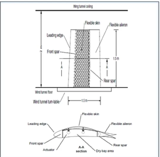
The prototype is a tridimensional wing with an internal structure manufactured in aluminum. The adaptive upper surface, composed of specially-designed composite materials, extends from 20% to 65% of the wing chord. The wing model is equipped with a rigid aileron situated at 72% of the chord, which will be replaced by a flexible one for test purposes. Four electrical actuators are disposed in two lines situated at 32% and 48% of the chord and are fixed on the central ribs. The actuators are controlled to push or to pull on the flexible skin to change the airfoil's shape. The cross section and the bottom view of the model used in the CRIAQ MDO-505 project are presented in Figure 1.3.
Figure 1.3 Cross section and bottom view of the MDO-505 wing model Taken from Koreanschi et al. (2015)
Aerodynamic optimizations of the wing airfoil were achieved by the LARCASE team at the ETS. The team conceived and developed an "in-house" methodology and code combining a genetic algorithm methodology and an Xfoil 6.96 open source aerodynamic solver (Koreanschi, Sugar et Botez, 2015). The objective of this optimization was to modify the initial airfoil shape of the prototype according to the flow conditions to obtain improved airfoil shapes that increase the wing’s laminarity. A 2D mathematical model (a B-splines representation) of the airfoil shape was morphed by means of two mobile control points, physically represented by the two actuators' lines on the wing. Figure 1.4 illustrates the wing airfoil section, showing the two mobile control points.
Figure 1.4 Wing airfoil section optimization Taken from Mamou et al. (2010)
The control points can be moved up and down on the airfoil during the optimization process, as shown in Figure 1.4. The optimization must result from the displacements of control points which are linearly adapted, via the control system, to find the true displacements of actuators. Various control architectures were developed within the LARCASE team to command the vertical displacements of the actuators (Kammegne, Botez et Grigorie, 2016). The IAR-NRC team was charged with the manufacture of the rigid wing prototype, while the ETS structure team was in charge of the design and manufacture of the flexible skin.
The experimental tests were conducted in the subsonic wind tunnel situated at the IAR-NRC laboratory. The design and manufacture of the morphing aileron took place in Italy, with the participation of Naples Frederico University II, Alenia and CIRA (the Italian Aerospace Research Center).
1.4 State of the Art: Numerical Prediction and Experimental Detection of the
Laminar to Turbulent Boundary Layer Transition
1.4.1 Boundary Layer Theory
In Fluid Mechanics, a fluid is characterized as "perfect" when it is possible to study its flow without considering its viscosity heat transfer. This kind of fluid does not exist in reality and
is generally only useful only for ideal mathematical representations. Let us consider a viscous fluid such as "air", which flows in front of a flat plate with a velocity equal to and that passes over the plate. Since the effect of viscosity is resistance fluid motion, the velocity of the fluid close to the solid plate continuously decreases downward and finally is equal to zero at the overlapping region between the fluid and the plate; that is, the "no slip condition". But, far from the flat plate, the flow speed remains equal to . Figure 1.5 shows the flow speed
variation over a flat plate.
Figure 1.5 Boundary layer of a flow over a plane plate
The flow speed diagram presents two distinct regions. The first is the region near the plate, where the flow speed decreases downwards due to the friction between the fluid and the plate. This first region is called the boundary layer. The second region, called the main flow, is outside the above region and is not affected by the friction. The boundary layer thickness is usually smaller than the main flow dimension, and is considered to be the distance from the flat plate surface to the point where the flow velocity reaches 99% of the main flow velocity. It depends on the non-dimensional Reynolds number.
In aerodynamics, the characterization of the flow over a wing within the boundary layer is an important factor, one with which both the wing lift and drag are quantified, as well as the evaluation of the heat transfer that occurs at high speeds. The boundary layer’s nature can be
laminar or turbulent depending on the value of the Reynolds number. For low Reynolds values, the boundary layer is laminar and is characterized by fluid particles flowing smoothly and constantly in parallel layers due to the viscous forces that are dominant to inertial forces. On the contrary, turbulent boundary layers exhibit the high property changes and random flow patterns that are associated with high Reynolds numbers. The flow transition occurs at a critical Reynolds number value Re lying between 2 × 10 and 3 × 10 , and is dependent upon the physical parameters of the tested model, such as the roughness and the curvature of the surface (Young et al., 2010).
The passage from laminar to turbulent boundary layer does not happen instantaneously, but requires a certain length in the direction of the flow. This length is called the "laminar to turbulent transition zone". The boundary layer of the flow generally starts in its laminar state and can transition to a turbulent state following different path, depending on the initial flow conditions, such as its disturbance amplitude and surface roughness (Saric, Reed et Kerschen, 2002). In fact, even a slight perturbation can progressively grow and turn the most laminar flow into a complex turbulent one.
For many years, the theoretical understanding of the boundary layer transition process did not really advance; most of its current understandings are based on experimental results. However, the gap between theory and experimental knowledge has recently been attenuated following several research efforts (White, 2006, p 439).
There are several assumptions regarding the flow transition in boundary layer theories; they may diverge sometimes, but most of them agree on the existence of different phases through which the fluid flow passes. The linear and weakly non-linear phases of flow transition were fairly well understood (Herbert, 1988; Kachanov, 1994). However, many questions still remain regarding the late non-linear transition phases (Kleiser et Zang, 1991). These different phases are known as:
- "Receptivity": This phase consists of the transformation of the outside disturbance into perturbations within the boundary layers. The initial disturbance, which is quite small (often unmeasurable) at the basic state of the flow, grows at varying rates depending on its nature and the basic state behavior. Perturbations such as Tollmien-Schlichting (Ts) waves or crossflow instabilities begin (Schlichting, 1968). The Ts waves' disturbance is one of the more common methods by which a laminar boundary layer transitions to turbulence. Their theory and evolution through the boundary layer were fully described in Smith and Gamberoni (1956).
- "Linear instabilities": In this phase, the perturbations that originate in the receptivity stage remain two-dimensional and small enough that the linear stability theory (Mack, 1984) can be used to describe their evolution.
- "Secondary instabilities" (non-linear growth and vortex breakdown to turbulence): The amplitude of the linear perturbations continues to increase until the perturbations turn into three dimensions, so that the linear theory can no longer be applied. Nonlinear instabilities are characterized by temporal and spatial incoherence of the flow, and an expansion of the frequency bandwidth that would rapidly lead to the occurrence of turbulent flow.
1.4.2 Numerical Prediction of the Boundary Layer Transition: N-factor Method
The first version of the e (later known as the e ) method for the semi-empirical prediction of the transition of two-dimensional incompressible boundary layers was first implemented by Van Ingen (1956). This approach, even though it is based on linear stability theory (Mack, 1984), has been used to predict the laminar to turbulent transition, which is definitely a nonlinear phenomenon. The method was able to calculate the amplification e of the unstable perturbation (such as Ts waves or CF instabilities) in the laminar boundary layer according to the following equation:
N(x, f) = A(x, f) A(x , f)
(1.1)
where N(x, f) represents the linear amplification of a given perturbation mode of frequency f, on a varying length − . The transition is supposed to start when any amplitude of any mode within the perturbation families reaches the threshold value (Crouch et Ng, 2000). The beginning of the transition is then located by the Equation 1.2:
max A(x, f) = A (1.2)
which means that the transition flow begins for a certain value of the N factor, given by equation 1.1 for A(x, f) = A .
For a good prediction of the flow transition on an airfoil, the N factor value needs to be calibrated, as it incorporates the receptivity and physical parameters of the model such as the surface roughness and the characteristic length. Mack, (1977) provided one of the earliest attempts to systematically model the variation of the N factor associated with Ts-wave transition. Mark's empirical equation relating the turbulence intensity to the N factor was written as follows:
N = −8.43 − 2.4 ln(T ) for 10 − 3 ≤ T ≤ 2.10 − 2 (1.3)
N factor method equations are implemented in many aerodynamic solvers, including Xfoil
software. Therefore, this is the approach that has been used for the numerical prediction of the boundary layer flow transition of the various aerodynamic profiles within the CRIAQ MDO-505 project, and which has been further tested in the IAR-NRC subsonic wind tunnel for experimental validation of the numerical simulation results.
1.4.3 Experimental Determination of the Boundary Layer Transition Region
Many flow visualization techniques have been developed over the years to clarify aerodynamic phenomena; for example, where shock waves occur or whether the flow is laminar, turbulent or transitional. In the absence of flow visualization, the transition process can be very difficult to explain. Methods using Schlieren photography (Bracht et Merzkirch, 1977), tufts (Crowder, 1980) and oil flow visualization (Loving et Katzoff, 1959) were and continue to be used in wind tunnel and flight tests.
These experimental methods for characterizing the boundary layer are always based on physical flow parameters and their properties (such as pressure, temperature, and viscous forces), and they are different for laminar and turbulent regimes. They each have their advantages and limitations.
1.4.3.1 Color Changes in Liquid Crystal Coatings
Originally discovered in 1888, the Liquid Crystal Method has been applied in the Aerospace industry for aerodynamic investigations in wind tunnel tests for boundary layer transition measurements. The method is based on the liquid crystal’s change of color when the liquid crystal is subjected to changes in shear stress, temperature or pressure. The color changes should be noticeable enough to differentiate a turbulent boundary layer from a laminar one (Holmes et al., 1986).
A complete review of the current thermochromic liquid crystal products was produced by Hallcrest, in which the chemical, physical and reference temperature bands were indicated for transition detection.
This transition detection method was applied by Holmes et al., (1986), in which they were able to visualize the laminar to turbulent boundary layer transition. When the liquid crystal coating was applied on the model, the coating needed to have a uniform thickness over the
whole model surface to obtain the maximum level of clarity in transition pattern development.
The method has the advantages that the changing color of the crystal coating is reversible and that its time response is under 0.2 seconds (Holmes et al., 1986), even though the performance of the airflow model can be affected by coating imperfections.
1.4.3.2 Oil Film Interferometry
The oil film interferometry method was theoretically proven and experimentally validated by Tannera and Blows, (1976). This method is based on the behavior of a silicon oil film placed on a surface and subjected to a flow. Tanner and Blows demonstrated that the evolution of the oil film motion during the experiment can only be related to the skin friction resulting from the flow boundary layer if the oil film remains thin enough (on the order of 10 μm). The product of "oil film thickness" and "time" becomes constant over time (for a given position of oil film on the model). The "oil film thickness" is measured using the "Fizeau interferometry technique", based on "laser ray reflection". The measuring procedure is fully described in Sykora and Holmes, (2011). The measured thickness of the oil film is representative of the skin friction over the surface model, allowing the distinction between the laminar and the turbulent boundary layers.
Oil film interferometry was successfully applied in several wind tunnel tests to characterize the boundary layer properties of models as part of the development of long-endurance aircraft designed to extend the laminar flow region for drag reduction (Drake, 2010).
This method presents advantages in terms of its low cost of materials and equipment, but the measuring procedure takes a relatively long time and is very sensitive.
1.4.3.3 InfraRed (IR) Thermography Visualization
Theoretically, laminar and turbulent boundary layers exhibit different behaviors in convective heat exchange. A turbulent boundary layer is marked by a transfer coefficient higher than the laminar one. The difference between the experimental model temperature and the flow temperature will attenuate more rapidly in a turbulent flow than in a laminar flow regime (Crawford et al., 2013). For example, a cold surface will heat faster under the influence of a turbulent boundary layer than in a laminar boundary layer. The principle of using InfraRed (IR) visualization for transition detection is based on this difference in the rate of the heat transfer characterizing a laminar versus a turbulent regime.
Generally, the initial temperature of the experimental model should be different than the flow temperature. To be assured of this initial difference, the experimental model could then be cooled or heated depending on the expected temperature of the flow, which should ideally remain constant over time. In this way, the temperature change of the model’s surface will largely depend on the heat transfer capacity of the flow, and thereby differentiate between the laminar flow and the turbulent regime.
The experimental setup for the IR visualization required two additional main components: an InfraRed camera and an insulator. The infrared camera was used to capture the temperature distribution along the model’s surface area. An insulator is required to eradicate any heat signature resulting from the model's components, which could be significant enough to overshadow any heat transfer occurring from flow effects, including flow transition (Joseph, Borgoltz et Devenport, 2014). The insulator should be smooth enough to preserve the model airfoil so that the aerodynamic performance is not altered. Joseph, Borgoltz, and Devenport (2014) used a coating (paint) as an insulator for the IR camera detection of the laminar to turbulent boundary layer in both wind tunnel and flight test environments.
The IR visualization technique has the advantage of being non-intrusive, as all of the equipment is external to the model, and therefore does not alter the airflow.
1.4.3.4 Second Derivative of the Pressure Distribution
Several methods for distinguishing the laminar from the turbulent regime are based on the pressure distribution of an airfoil.
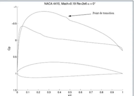
Popov et al., (2008) theoretically and experimentally demonstrated that the transition zone can be localized by detecting the pressure step increase in the pressure distribution. This pressure step increase had earlier been identified and explained by Galbraith and Coton (1990) as representing the separation bubble that appears in the boundary layer during the flow transition process. Figure 1.6 shows a pressure distribution on the NACA 445 airfoil predicted by Xfoil software, in which the predicted transition zone is visible as an increase in the pressure step (Popov, Botez et Labib, 2008).
Figure 1.6 Pressure distribution of a NACA 4415 profile for a Mach number
of 0.19, a Reynolds number of 2e6 and an angle of attack of 0 degrees (Popov et al., 2008)
The method proposed by Popov, Botez and Labib (2008) has shown that the maximum of the second derivative of the pressure distribution with respect to x corresponds to the maximum curve of the pressure plot, which represents the beginning of the transition.
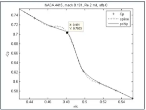
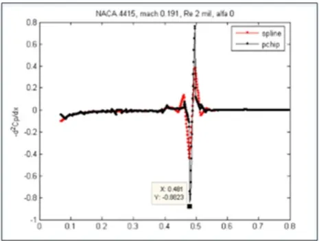
To experimentally verify their theory, Popov, Botez and Labib (2008) designed a NACA 4415 airfoil wing, for which the upper surface of the model was equipped with 84 pressure sensors, so that the pressure distribution could be detected with sufficient accuracy. Both the Spline and the PCHIP (piecewise cubic Hermite interpolating polynomial) (Hussain and Sarfraz, 2009) methods were used for interpolation between the local points recorded by the sensors before applying the second derivative method. Figure 1.7 and Figure 1.8 show an interpolated Cp distribution of the NACA 4415 airfoil and second derivative of its pressure distribution respectively, wherein the maximum second derivative value is identified at 48.1% of the chord.
Figure 1.7 Pressure coefficient distribution in the vicinity of the transition point interpolated using the Spline and PCHIP methods.
Figure 1.8 Second derivative of the pressure coefficient distribution interpolated using the Spline and PCHIP methods.
Taken from Popov et al., (2008)
This method has a huge advantage in that it can detect the transition in real time, but it requires a significant number of pressure sensors to obtain a high level of accuracy, which can be a practical disadvantage for a model with a large area.
1.4.3.5 Pressure Distribution Spectral Analysis
While Popov, Botez and Labib (2008) focus on deviations of the mean pressure over the total wing chord, the spectral analysis method considers the recorded pressure fluctuations over time to evaluate which sensors belong to the laminar and which to the turbulent zone. The pressure fluctuations are expected to be more intense in a turbulent flow than in a laminar one (Parameswaran and Jayantha, 1999), due to the amplification of the nonlinear perturbations occurring during the transition. Therefore, this method mainly utilizes the difference in pressure fluctuations to determine the transition area.
The pressure fluctuations are visualized and quantified by means of Fast Fourier Transforms (FFT) (Mathworks, 2006) and Standard Deviation (SD) algorithms (Mathworks, 2006) applied on the recorded data. This approach was applied by (Popov et al., 2010) to experimentally determine the transition area of several optimized airfoils for multiple wind tunnel tests during the CRIAQ 7.1 morphing wing project. Their model was equipped with 16 Kulite piezoelectric sensors, capable of sensing high frequency fluctuations of up to 10 KHz. The Kulite transducers present many other advantages, such as their relatively small size and their very precise and accurate measurements and accuracy. Thirty-six optimized airfoils for drag reduction were found for the flight cases expressed by combinations of Mach numbers 0.2, 0.225, 0.25, 0.275, 0.3 and angles of attack -1, -0.5, 0, 0.5, 1 and 2 degrees (Popov et al., 2010).
The good correlation between the experimental methods and the Xfoil numerical simulations results obtained during the CRIAQ 7.1 project led to the choice of the pressure distribution spectral analysis for the experimental determination of the laminar to turbulent transition area in the CRIAQ MDO 505 project.
1.5 Aeroelastic Behavior and Vibration Measurements of a Wing
1.5.1 Aeroelastic Behavior
Flight and wind tunnel testing on wing models always involve some vibrations studies, as vibrations should be minimized, not only to preserve the wing's aerodynamic performance, but also to ensure the safety of all the operators around the model. Courchesne, Popov and Botez (2010) performed aeroelastic studies to avoid possible flutter occurrences during wind tunnel testing on a morphing wing model. Their analysis showed that the wind tunnel tests could be performed safely because aeroelastic instabilities for the studied morphing configurations could only occur at Mach number 0.55, which was higher than the wind tunnel Mach number limit speed of 0.3.
Flore and Cubillo (2015) studied the dynamical behavior of an aircraft wing structure. They analyzed the change of the dynamic behavior of the wing structure relative to the applied loading to simulate real aircraft operating conditions. During experimental tests, they proved that both strain gages and accelerometers could be used for vibration sensing with satisfactory results.
1.5.2 Strain Gages
Omega Engineering, (2000) defines a strain gage as a device for indicating the strain of a material or structure at the point of attachment. It uses the change in electrical resistance to measure strain when it is subject to mechanical motions. Strain gages can have several applications, such as in shock analysis and vibration measurements. The displacement measurements are accomplished by using the proportional relation between the deflections of a loaded mechanical member and the strains at every point in the member, as long as all strains are within their elastic limits. Wilson, (1976) gave a complete review of strain gage instrumentation at that time. Strain gage theory and applications have been widely represented. Pisoni et al. (1995) and Burrows (1975) used strain gage equipment for the real time determination of displacements at various points of a vibrating body; this information could be especially valuable for position control measurements of aeroelastic systems.
1.5.3 Accelerometers
Accelerometers are sensors that measure the acceleration of the body they are installed on. Such a device can be used for many applications, including tilt sensing (Chendjou et Botez, 2014), shock quantification (Broch, 1980), and vibration measurements (McFadden et Smith, 1984). Several types of accelerometers are available. The most common types are piezoelectric and Micro Electro-Mechanical System (MEMS) accelerometers.
Albarbar et al., (2009) provided detailed information about MEMS accelerometers performance, describing the devices high level of performance despite their relatively low
cost. MEMS accelerometers were therefore selected for use in the CRIAQ MDO-505 project to sense and measure vibration data for the experimental validation of aeroelastic studies on the model (Koreanschi et al., 2016).
CHAPTER 2
PRESSURE DATA ACQUISITION SYSTEM AND POST PROCESSING METHODOLOGY
2.1 Context
One of the main objectives of the MDO 505 project was to improve the aerodynamic performances of a morphing wing prototype by delaying the occurrence of the laminar to turbulent boundary layer transition zone. The success of the experimental tests in the IAR-NRC wind tunnel relied on the validation of the numerical predictions. This validation necessitated an accurate experimental characterization of the airflow, which includes both a reliable data acquisition system and reliable post-processing methods, as well as correct interpretations of the post-processed results. The frequency analysis method of the pressure distribution airflow was chosen for detecting the transition zone location at the chord situated at 40% of the wing span. The sensors' measurements should be accurate enough to determine the pressure distribution over this wing section airfoil, and they should have a sufficiently large bandwidth to capture the pressure fluctuations resulting from the Tollmien-Schlichting waves. The Infra Red thermography visualization over the wing surface was used as supplementary method to detect the transition over the whole wing span. A wind tunnel balance was also used to evaluate the load variations (lift, drag, moments) resulting from the morphing procedure.
This chapter first fully describes the wing model. This is followed by a description of the real time acquisition system equipment, as they are used to gather the pressure data. The description focuses on the pressure sensors and their characteristics. Next, the post processing procedures for obtaining the Cp distribution profile and for determining the laminar to turbulent boundary layer transition are detailed. The interpretation of a sample case is presented to clarify the procedure. More results are displayed in Chapter 4.
2.2 Description of the Wing Model
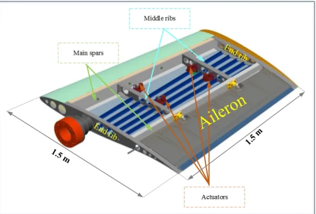
The wing model had the dimensions of a real aircraft wing tip (wing and aileron), provided by Bombardier (one of the project's partners), which was representative of their type of transport aircraft and capable of withstanding 1g in-flight loads. The wing prototype measured 1.5 meters for its span, and its root chord was also 1.5 meters, with a taper ratio of 0.72 and a leading edge sweep angle of 8 degrees. The adaptive upper skin, designed and optimized from carbon material composite, was situated between 20% and 65% of the chord. Figure 2.1 presents the wing-tip model dimensions and its internal structure.
Figure 2.1 Internal structure of the wing model
The wing's internal structure was mainly manufactured from Aluminum and had four ribs, two main spars and two secondary spars (showed in blue on Figure 2.1), reinforcing the lower and upper skins. The wing's flexible upper skin was manufactured from composite materials (Michaud, Joncas et Botez, 2013). It therefore had the capacity of changing its
shape in order to efficiently withstand different load conditions. To realize the desired shape changing, four electrical actuators distributed along two lines (32% and 48% of the chord) were installed inside the wing. The actuators were supported by the two middle ribs, which acted as embedment supports. The two ends ribs and spars ensured a satisfactory rigidity of the wing, as required by industry specifications, despite its flexibility.
2.3 Real Time Acquisition System for Pressure Measurements: Kulite
Transducers Setup and their Installation on the Wing.
The sensors used for the pressure distribution and for flow transition detection during the wind tunnel tests were ultra-miniature Kulite XCQ-062 pressure transducers. They are manufactured and distributed by Kulite Semiconductor. The Kulite XQC-062 transducers measure the differential pressure between two pressure points of the system. The first point is the local pressure on the model and the other is the referenced static pressure of the Wind Tunnel test section. This differential pressure is then proportionally converted into a displacement by using a force-summing device over a wide range of frequencies. The displacement is in turn, applied to an electrical transducer element (composed of a Wheatstone bridge plus a temperature compensator) in order to generate the required electrical output signal. Figure 2.2 presents a graphical representation of the Kulite XCQ-062 transducer as well as a photographic image.
Figure 2.2 Graphical representation of Kulite XCQ-062 transducer (Annex I) Adapted from Kulite Semiconductor (2014)
The force-summing device and the transducer element are physically combined into a micro-machined dielectrically isolated silicon diaphragm of dimensions 1.5 mm *9.5 mm, which has a reliable stiffness and a negligible mass. This diaphragm confers excellent properties to the Kulite sensors such as a wide frequency response, high sensitivity and immunity to acceleration and strain inputs, as seen in Annex I.
To install the Kulite sensors on the upper skin of the model, holes of 1.7 ± 0.005 mm were made on its surface, and sensors were perpendicularly set from the inside to the outside of the wing, ensuring that the sensors' extremities were aligned with the composite skin surface, as shown on Figure 2.3.
Figure 2.3 Sketch of a Kulite sensors installation on the composite skin
The sensors' positions were reinforced by using an adhesive (shown in yellow on Figure 2.3) to keep it fixed despite the vibration that generally occurs during the wind tunnel tests. Figure 2.4 displays the inside surface of the composite skin of the wing; the yellow circles indicate where the pressure sensors are installed.
Figure 2.4 Inside surface of the composite skin
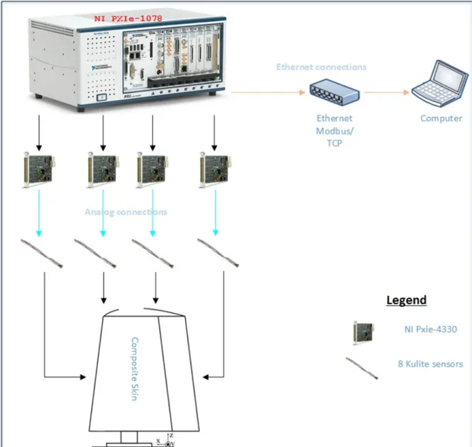
The real time acquisition system for Kulite pressure measurements was composed of a NI PXIe-1078 chassis equipped with a central processing unit, four NI PXIes-4330's each capable of handling eight analog inputs, with a sampling rate of up to 25,000 samples per second for each channel. A personal computer was also connected via an Ethernet network to the NI PXIe-1078 to monitor the data and handle their real-time visualization. Finally, a voltage source supplied the NI systems and the Kulite transducers. The connections between the different components are shown in Figure 2.5.
Figure 2.5 Overview of the pressure data acquisition system and connections between the components
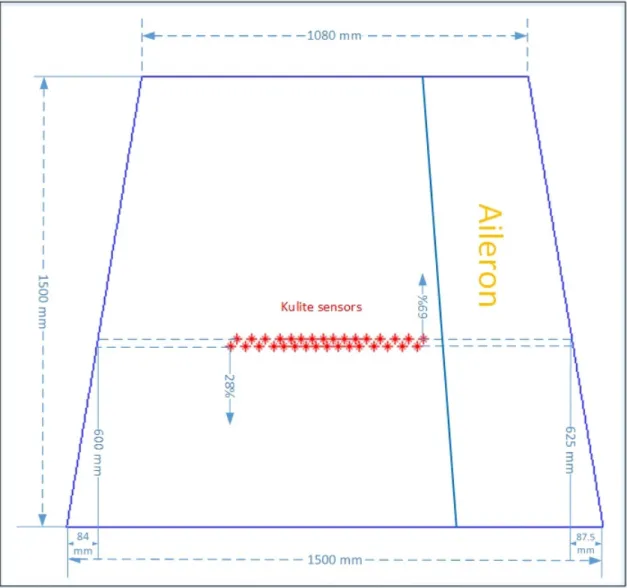
Thirty-two Kulite sensors were installed on the wing model. They were disposed on the upper skin surface along two chord lines situated at 600 mm and 625 mm from the wing root, between 28% of the chord and 69% of the chord. Two successive sensors had a minimum distance between them of 30 mm and a maximum distance of 40 mm in order to avoid interferences, but also to minimize their pressure information losses. Figure 2.6 shows the representation of the Kulite sensors' disposition on the wing-tip.
Figure 2.6 Representation of the wing dimensions and Kulite sensors distribution on the composite skin surface
Each Kulite sensor was therefore positioned at a percentage of chord, as presented in Table 2.1
Table 2.1 Chord percentage at which Kulite sensors are positioned on the wing Sensor #1 : 28.5 % Sensor #17 : 51.2 % Sensor #2 : 29.5 % Sensor #18 : 52.6 % Sensor #3 : 33.4 % Sensor #19 : 53.5 % Sensor #4 : 35.2 % Sensor #20 : 54.6 % Sensor #5 : 36.3 % Sensor #21 : 55.7 % Sensor #6 : 37.5 % Sensor #22 : 56.9 % Sensor #7 : 38.2 % Sensor #23 : 57.2 %
Table 2.1 (continued) Sensor #8 : 39.1 % Sensor #24 : 58.7 % Sensor #9 : 41.3 % Sensor #25 : 60.2 % Sensor #10 : 42.4 % Sensor #26 : 61.5 % Sensor #11 : 43.6 % Sensor #27 : 62.8 % Sensor #12 : 44.3 % Sensor #28 : 63.8 % Sensor #13 : 45.2 % Sensor #29 : 65.4 % Sensor #14 : 46.2 % Sensor #30 : 66.0 % Sensor #15 : 50.0 % Sensor #31 : 67.7 % Sensor #16 : 50.8 % Sensor #32 : 68.3 %
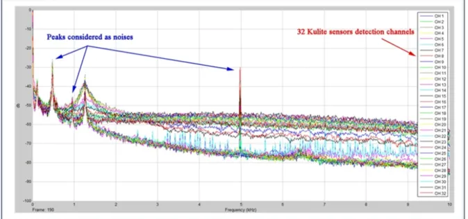
The Kulite sensors outputted differential pressure variations from 0 to 5 PSI in terms of tension, with a sensitivity of 20mv/PSI. These sensors also had an infinitesimal resolution and a natural frequency range of 150 KHz. The analog signal was conditioned by means of an anti aliasing filter incorporated in the NI PXIe-1078 chassis. The resulting output signal was sampled at the rate of 20 KHz, so that the pressure fluctuations from 0 to 10 KHz could be visualized through Fast Fourier Transform (FFT) representation. This rate was high enough to capture the nonlinear instabilities that occurred during the transition process. In fact, following the Nyquist-Shannon theorem (Bellanger et al., 2013), the sampling rate should at least be twice the highest frequency of the desired visualized signal for an accurate conversion of analog to discrete signals.
2.4 Numerical Aerodynamic Optimization and Prediction of the Performances of
the Wing Airfoil
Before performing wind tunnel tests, the optimized airfoils for the various flight conditions were obtained by using a genetic algorithm developed 'in-house' (Koreanschi, Sugar-Gabor et Botez, 2014). Subsequently, numerical predictions of both the pressure coefficients and the transition area of the multiple airfoil configurations were achieved by using the Xfoil 6.96 open source aerodynamic solver, which were further confirmed using Fluent software. The prediction of the transition area through the Xfoil solver was based on the N-factor method described in section 1.4.2. Simulations on the Xfoil solver required the several parameters,
such as the coordinates of the airfoil we wanted to analyze, the Mach number, the angle of attack, the deflection angle of the aileron and the Reynolds number.
Ninety seven (97) different flight configurations were simulated, optimized for transition delay and further tested at the IAR-NRC wind tunnel for validation of their simulation results. Mach numbers of 0.15, 0.2 and 0.25 were considered as airspeeds. The angle of attack varied from −3 to 5 , while the aileron deflection angles changed from −6 to 6 . The Reynolds number was calculated from the air characteristics and the model dimensions (length ), as shown in equation 2.1:
= (2.1)
Where,
- = 1.225 Kg. m is the air density of air at the wind tunnel test conditions - is the airspeed which depends on the flight test configuration chosen
- = 1.32 m is the characteristic length, which is equal to the length of the sensors chord line; and
- = 1.80 ∗ 10 Kg. m . s is the dynamic viscosity of the air.
Eighteen of the ninety-seven fight configurations are summarized in Table 2.2.
Table 2.2 Tested cases optimized for laminar flow improvement Flight case
number Mach Number Angle of attack Aileron deflection Reynolds number
15 0.15 -0.5 6 4.67 18 0.15 -2 -2 4.62 25 0.15 1.5 -2 4.66 38 0.25 0.5 -1 7.77 40 0.15 1 0 4.67 41 0.15 1.25 0 4.66 42 0.15 1.5 0 4.65
Table 2.2 (continued) 43 0.15 2 0 4.64 44 0.15 2.5 0 4.65 45 0.15 3 0 4.66 47 0.15 -2.5 2 4.66 68 0.2 0 4 6.22 69 0.2 0.5 4 6.23 70 0.2 1 4 6.23 71 0.2 1.5 4 6.22 72 0.2 2 4 6.25 80 0.2 3 -4 6.19 82 0.2 5 -4 6.18
2.5 Description of the Wind Tunnel Post Processing Procedure
The waveforms recorded during the wind tunnel tests contained pressure data from the 32 different sensors installed on the composite skin (Figure 2.3). The data were recorded at the rate of 20 KHz for each sensor channel, and the recording procedure was repeated for ninety-seven different flight configurations on the morphing wing and on the un-morphed wing. The data were processed and further interpreted with the aim of validating the numerical simulation results by comparing them to the pressure coefficient distributions resulting from wind tunnel data. An evaluation of the backward motion of the transition area as a positive effect of the applied morphing was also performed.
2.5.1 Pressure Coefficient Distribution
For the generation of the pressure coefficient distribution over the wing airfoil, conventional pressure tab sensors were used to record static pressure measurements on the rest of the wing section (inner surface and aileron), since the Kulite sensors were only installed on the composite skin upper surface.
The pressure coefficient for each sensor is computed from the row data by using equation 1.4:
= 1 2
(2.2)
where Δ is the mean pressure of each sensor recorded data, is the air density and is the flow velocity. Figure 2.7 presents a comparison between the numerical and experimental pressure coefficients for the wing section located at 40% of the span (Kulite sensor line chord), for flight case #15 (Mach=0.15, α=-0.5˚, δ=6˚).
Figure 2.7 Comparison of the numerical versus the experimental pressure coefficient distribution for flight case #15; original airfoil (left) and optimized airfoil (right) From Figure 2.7, an acceptable similarity between the 2D numerical predictions and the wind tunnel tests results can be observed for flight case #15 (Table 2.2). As expected, a very good agreement is observed between the 3D numerical and the experimental pressure values. The influence of the surface change due to morphing can be clearly observed from the original to the optimized airfoil pressure coefficients, measured on the interval situated between 28% and 68% of the chord (Kulite sensor region is represented in "green" in Figure 2.7). In fact, the skin morphing extends the wing upper surface laminar region where the air accelerates, and therefore generates more favorable conditions for laminar flow. This effect is clearly visible on the left and right hand sides of Figure 2.7.