Knowledge acquisition within an organization: How to retain a knowledge worker using wage profile and non-monotonic knowledge accumulation

Texte intégral

(1)2014s-32. Knowledge acquisition within an organization: How to retain a knowledge worker using wage profile and non-monotonic knowledge accumulation Ngo Van Long, Antoine Soubeyran, Raphael Soubeyran. Série Scientifique Scientific Series. Montréal Juin 2014. © 2014 Ngo Van Long, Antoine Soubeyran, Raphael Soubeyran. Tous droits réservés. All rights reserved. Reproduction partielle permise avec citation du document source, incluant la notice ©. Short sections may be quoted without explicit permission, if full credit, including © notice, is given to the source..

(2) CIRANO Le CIRANO est un organisme sans but lucratif constitué en vertu de la Loi des compagnies du Québec. Le financement de son infrastructure et de ses activités de recherche provient des cotisations de ses organisations-membres, d’une subvention d’infrastructure du Ministère de l'Enseignement supérieur, de la Recherche, de la Science et de la Technologie, de même que des subventions et mandats obtenus par ses équipes de recherche. CIRANO is a private non-profit organization incorporated under the Québec Companies Act. Its infrastructure and research activities are funded through fees paid by member organizations, an infrastructure grant from the Ministère de l'Enseignement supérieur, de la Recherche, de la Science et de la Technologie, and grants and research mandates obtained by its research teams. Les partenaires du CIRANO Partenaire majeur Ministère de l'Enseignement supérieur, de la Recherche, de la Science et de la Technologie Partenaires corporatifs Autorité des marchés financiers Banque de développement du Canada Banque du Canada Banque Laurentienne du Canada Banque Nationale du Canada Banque Scotia Bell Canada BMO Groupe financier Caisse de dépôt et placement du Québec Fédération des caisses Desjardins du Québec Financière Sun Life, Québec Gaz Métro Hydro-Québec Industrie Canada Intact Investissements PSP Ministère des Finances et de l’Économie Power Corporation du Canada Rio Tinto Alcan Transat A.T. Ville de Montréal Partenaires universitaires École Polytechnique de Montréal École de technologie supérieure (ÉTS) HEC Montréal Institut national de la recherche scientifique (INRS) McGill University Université Concordia Université de Montréal Université de Sherbrooke Université du Québec Université du Québec à Montréal Université Laval Le CIRANO collabore avec de nombreux centres et chaires de recherche universitaires dont on peut consulter la liste sur son site web. Les cahiers de la série scientifique (CS) visent à rendre accessibles des résultats de recherche effectuée au CIRANO afin de susciter échanges et commentaires. Ces cahiers sont écrits dans le style des publications scientifiques. Les idées et les opinions émises sont sous l’unique responsabilité des auteurs et ne représentent pas nécessairement les positions du CIRANO ou de ses partenaires. This paper presents research carried out at CIRANO and aims at encouraging discussion and comment. The observations and viewpoints expressed are the sole responsibility of the authors. They do not necessarily represent positions of CIRANO or its partners.. ISSN 2292-0838 (en ligne). Partenaire financier.

(3) Knowledge acquisition within an organization: How to retain a knowledge worker using wage profile and nonmonotonic knowledge accumulation Ngo Van Long *, Antoine Soubeyran †, Raphael Soubeyran ‡. Résumé/abstract Dans ce papier, nous considérons un problème d'accumulation de connaissances dans une organisation. Nous partons de la théorie du capital humain lancée par Becker (1962, 1964) et considérons une organisation qui ne peut pas empêcher un employé de quitter et d’utiliser la connaissance à l'extérieur de l'organisation. Nous montrons comment l'employeur manipule de façon optimale le sentier d'accumulation de connaissances et choisit un profil de salaire pour atténuer le problème d'engagement. Nous montrons que l'accumulation de connaissances est retardée : la fraction de temps alloué à la création de connaissances est la plus haute au premier stade de la carrière, puis elle tombe progressivement, ensuite, elle monte de nouveau, avant de tomber finalement vers le zéro. Nous déterminons l'effet de la spécificité de connaissances. Nous discutons aussi la forme des profils de salaire optimaux, le rôle du niveau de connaissance initial et du rôle du fait du taux d’actualisation. Mots clés : Capital humain, hold-up, contrat.. In this paper, we consider a knowledge accumulation problem within an organization. We depart from the human capital theory initiated by Becker (1962, 1964) and consider an organization that cannot prevent the worker from quitting and using the knowledge outside the organization. We study how the employer optimally distorts the knowledge accumulation path and chooses a wage profile in order to mitigate the commitment problem. We show that knowledge accumulation is delayed: the fraction of working time allocated to knowledge creation is highest at the early career stage, falls gradually, then rises again, before falling finally toward zero. We determine the effect of a change in the severity of the enforcement problem (or the specificity of knowledge). We also discuss the form of the optimal lifecycle wage profiles, the role of the initial knowledge level and the role of discounting Key words: Human capital,hold-up, contract Codes JEL : J2. *. CIRANO, and Department of Economics, McGill University. Email: ngo.long@mcgill.ca Aix-Marseille University (Aix-Marseille School of Economics), CNRS & EHESS. Email: Antoine.soubeyran@univ_amu.fr ‡ INRA, UMR1135 LAMETA, F-34000 Montpellier, France. Email: soubeyra@supagro.inra.fr †.

(4) Introduction One of the main issues in leading knowledge workers is how to retain them in the …rm, as monetary incentives alone are often not su¢ cient. The nature of the tasks given to knowledge workers are an important incentive to retain them in the …rm (Prince, 2011). Companies often propose new tasks to their knowledge workers, and academic departments of research-oriented universities assign teaching loads and administrative responsibilities (that constraint research time) that vary along the career path.1 The human capital theory initiated by Becker (1962, 1964) and Mincer (1958, 1962, 1974) has o¤ered a rich analysis of an individual’s life cycle investment in human capital. One of the main results of this literature states that human capital investments are undertaken at the early stage of the career because workers have then a longer period of time over which they can bene…t from the return of their investments. Becker’s focus on the investment demand side has been complemented by supply-side considerations o¤ered by Ben-Porath (1967), who assumed that an individual must allocate a fraction of his human capital as an input, to be combined with purchased inputs, in his investment in human capital. Ben-Porath showed that this fraction is changing over time, and generally it becomes smaller and smaller as the individual approaches the retirement age.2 Both the Becker mechanism and the Ben-Porath mechanism predict that for any individual the investment in human capital declines over time. In this paper, we consider a di¤erent mechanism that, unlike the other two previous mechanisms, is capable of producing a non-monotone path of investment in human capital. The driver behind our result is the role of the employer, who actively o¤ers the knowledge workers time-varying …nancial and non…nancial incentives to stay with the …rm. In the …rst best situation, where the employer and the knowledge worker can sign binding contracts, we show a result similar to the standard human capital theory, i.e., the share of time allocated to knowledge creation decreases over time. In the second-best situation, where the knowledge worker can leave the organization and use the accumulated knowledge to earn income outside the organization, we show that the time path of investment in human capital can be non-monotone. At the beginning of her career, the worker is asked to spend a large share of her time to knowledge creation, but gradually she is asked to allocate an increasing share of time to routine tasks. Around the middle of her career, this trend reverses and the employer allows the knowledge worker to devote more and more time to knowledge creation. Toward the end of her career, the trend reverses again and the knowledge worker is asked to perform more and more routine tasks. Our main result …ts well with the existing evidence on life-cycle human capital accumulation pro…les. Human capital accumulation being di¢ cult to measure, the empirical literature provides mainly documentation of formal on-the-job training. The available evidence is consistent with our result that human capital 1 For. instance, Google’s engineers can work 20% of their time on independent projects. made the distinction between observed earnings and earnings net of all investment costs: the former are always higher, change slowly, and peaks at an earlier date than the latter. 2 Ben-Porath. 2.

(5) accumulation is not concentrated at the beginning of the career. Indeed, Loewenstein and Spletzer (1997) show that delayed formal training (i.e. an increasing quantity of formal training over time) is frequent. This empirical result suggests that human capital investments are not undertaken without delay, at the early stage of the career. In contrast to the presumption of concentrated accumulation of human capital at the beginning of the career, our main result shows that …rms prefer some delay in human capital investments in order to retain the worker (this point will be further discussed in section 5). After establishing our main result, we discuss the e¤ect of a change in the severity of the enforcement problem (or the speci…city of knowledge). We show that an increase in the enforcement problem (or a decrease in the degree of …rm-speci…city of knowledge) decreases the share of working time allocated to knowledge creation and decreases cumulated knowledge. Somewhat surprisingly, an increase in the di¢ culty of enforcement can increase or decrease the life-time income of the knowledge worker. Consistent with Ben-Porath (1967), our model is able to generate the main feature of age-earnings pro…les (e.g. Heckman 1976, Rosen 1976, and Murphy and Welch 1990), namely, the experience-earnings pro…le is a hump-shaped function of experience. We also discuss the returns to schooling in our model (see Heckman et al. 2003 and Belzil 2007 for surveys of the literature). We show that our main result is robust to an increase in the initial knowledge level. And, consistently with recent evidence that di¤erences in lifetime earnings are mainly due to initial conditions (see Hugget et al. 2011), we show that an increase in the initial knowledge level has a positive e¤ect on earnings. The paper is organized as follows: Section 1 presents the model and notations; in Section 2 we derive the …rst best knowledge accumulation path; in Section 3, we show how an employer retains a knowledge worker using wage pro…le and delayed knowledge accumulation. We also discuss the shape of the optimal wage pro…le and show how a change in the severity of the enforcement problem a¤ects our results. In Section 4, we focus on the role of the initial knowledge level, the role of the discount rate, and show that our results remain valid in the case of a strictly concave utility function. Section 5 discusses the link between our model and the empirical evidence. In Section 6, we relate our model to several strands of the literature. Section 7 concludes.. 1. Model and notations. The time horizon T represents the maximal career duration of the employee. Each period, the employee is endowed with a …xed working time (normalized to 1) to be split between time spent to create knowledge, k ( ), and time spent on the usual task, l( ). The time constraint of the employee is k ( ) + l( ) = 1. The Rt employee’s cumulated knowledge at any time t is K (t) = 0 k ( ) d . Inside the …rm, the pro…t at time. generated by the employee’s cumulated knowledge is denoted by. 3.

(6) (K ( )) with. (0) = 0,. 0. 00. > 0 and. 0.. We make a natural assumption concerning outside options: if the employee leaves the …rm at time tl , her expected future revenue (per period) is an increasing function of the stock of knowledge cumulated up to tl . Moreover, following Becker (1962), we distinguish two categories of human capital, speci…c and general human capital. Speci…c human capital is related to a speci…c …rm’s products or services whereas general human capital can be used in a large range of di¤erent …rms. Accordingly, the employee’s earning outside the …rm will be ^ (K (tl )), where we assume that ^ (K) is more useful inside the …rm than outside and 1. 2 (0; 1).3 In other words, knowledge. ( K), with. represents the degree of speci…city of knowledge. The. employee who quits at tl receives ( K (tl )) each period of time. > tl outside the …rm, using the knowledge. cumulated up to tl . After the employee quits, the …rm obtains a constant value (normalized to 0) each remaining period of time. As long as the employee remains with the …rm, it earns the pro…t (K( )), and an additional amount v (l ( )) if the employee spends a fraction l( ) of her time endowment on routine tasks. Assume that for all l 2 [0; 1], v (l) discount rate r ( K ( )). 0, non-decreasing, and strictly concave. The employee and the employer have the same 0. Under our assumptions, the surplus of the relationship at time. is. (K ( )) + v (l ( )). 0.. At time t = 0, the employer and the employee sign a contract. The contract speci…es the fraction k( ) of working time that must be devoted to knowledge creation, the remaining fraction l ( ) being allocated to the routine task,. 2 [0; T ], and a wage pro…le represented by w ( ) for. 2 [0; T ]. Thus, if the employee. quits at time tl , the cumulated payo¤ of the employee over the lifetime horizon is:. Vw =. Ztl. e. r. w( )d +. ZT. e. r. ( K (tl ))d ;. tl. 0. 4. and the cumulated payo¤ of the employer is Vf =. Ztl. e. r. [ (K ( )) + v (l ( ))] d. 0. Ztl. e. r. w( )d :. 0. Notice that our model does not include other possible payo¤s such as the knowledge worker’s egorent, or her pleasure obtained from knowledge creation. Adding such factors would make the model more cumbersome, without changing our main results. 3 Our main results are not a¤ected if we instead consider the more general assumption that ^ is an increasing and concave function of K, such that ^ (K) (K). 4 Despite we assume additivity, notice that a multiplicative form of the instantaneous payo¤ is compatible with our model. If one chooses (:) v (:) ln (:), the instantaneous payo¤ from working (K) + v (l) can be written in the multiplicative form ln (K l).. 4.

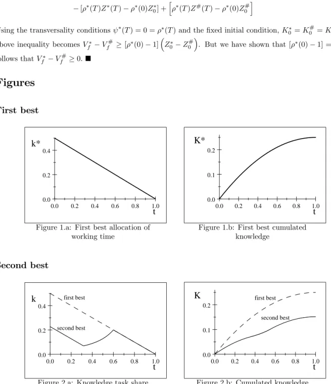
(7) 2. First best solution. If the employee leaves the …rm at time tl J (tl ) =. Ztl. e. r. T , the joint surplus over the time horizon T is given by. [ (K ( )) + v (l ( ))] d +. ZT. e. r. ( K (tl ))d ;. tl. 0. where k ( ) + l( ) = 1. The opportunity cost of time devoted to the knowledge task can be written as v (l( )) = v (1. 0 tl. k ( )). The joint surplus optimization programme can then be written as 9 8 Ztl ZT = < ; J (tl ) = e r [ (K ( )) + v (1 k ( ))] d + e r ( K (tl ))d max ; T; 0 k( ) 1 : tl. 0. where 0. k( ). 1,. and subject to _ ) = k( ); K( and, K(0) = 0 (given). Clearly, since ( K). (K) for all K. 0 and since v(1. k). 0 for all feasible k 2 [0; 1], the solution. of the joint surplus maximization problem displays the plausible property that the two parties stay together until T . Another property of the solution concerns the fraction of time devoted to knowledge creation: it is decreasing over time. This is described in the following proposition.5 Proposition 1 [First best allocation of time between tasks]: The optimal duration of the relationship is tl = T and the optimal (interior) splitting of working time is such that the share of time allocated to knowledge accumulation is decreasing whereas the share of time allocated to the routine task is increasing (k_ < 0 and l_ > 0). The joint surplus maximization requires that the share of working time allocated to the knowledge task decreases over time and the share of time allocated to the routine task increases over time. In other words, the share of the routine task is gradually becoming dominant. Knowledge is accumulated mainly at the beginning of the career because the sooner the investment in the knowledge task, the larger the cumulative bene…ts. When the employee approaches the end of the horizon, knowledge accumulation becomes less attractive because there is less remaining time to exploit knowledge. Indeed, the shadow price of knowledge, RT 0 , decreases through time, (t) = t 0 (K ( )) e r d and _ (t) = (K (t)) e rt < 0. Let us illustrate this result with an example:. 5 All. proofs are relegated to the Appendix.. 5.

(8) Example 1: Let us specify the functions as follows. assume that AT. (K) = AK with A > 0 and v (l) = l. 1 2 2l .. We also. 1 which ensures the existence of an interior solution. (For the Figures, we set T = 1;. A = 1=2). In this example, we have k ( ) = A (T. ) and l ( ) = 1. A (T. ).. [INSERT FIGURES 1a,b] The …rst best solution is based on the assumption that both parties can commit to continuing their relationship until T . However, since the employee is accumulating knowledge, the value of her outside income ( ( K)) is increasing over time, hence if the employee is free to quit at any time, she would have an incentive to quit unless the employer promises her su¢ cient reward for staying with the …rm. This reward can come in two forms: a monetary reward, such as a time pro…le of salary that evolves with seniority, or a prospect of accelerated increase in human capital in the future (which tilts the time path of her outside option toward the future). The next section investigates this issue.. 3. How to retain a knowledge worker using wage pro…le and nonmonotonic knowledge accumulation. We now consider the situation where the knowledge worker can quit at any time t 2 (0; T ), taking with her the knowledge that she has acquired while being employed. We derive the properties of the optimal splitting of working time when the employer designs a scheme that prevents the knowledge worker from quitting the …rm before the retirement age T . The …rm has two instruments to retain the worker: it prescribes a time path of allocation of working time between knowledge creation and the routine task, and it gives a monetary payment to the knowledge worker. An interesting feature of our model is the optimal trade o¤ (from the …rm’s vantage point) between these two instruments. For simplicity, we assume that both the employer and the employee do not discount the future, r = 0. We will relax this assumption in sub-section 4.2 and show that our main result is not a¤ected: the optimal splitting working time remains non-monotonic. The knowledge worker receives a non-negative wage, w ( ), at time . We assume that the …rm cannot ask the worker to post a bond and it cannot ask her to pay any compensation once she has left. From time t, if RT the worker stays with the …rm up to T she enjoys a cumulated wage W (t) w ( ) d . If she chooses to leave t. the …rm at time t, her payo¤ for the remaining working life is R (t). RT. ( K (t))d = (T. t) ( K (t)). It is. t. important to notice that the value of her outside option, denoted by R (t), evolves through time. The worker will not quit before the time horizon T if the …rm o¤ers her a contract such that the following non-quitting constraint is satis…ed: W (t). R (t) for all t 2 [0; T ] :. The problem to be solved by the employer can then be written as follows:. 6. (1).

(9) max. 0 k( ) 1; 0 w( ). Z. T. [ (K( )) + v(1. k( )). w ( )] d. (2). 0. subject to _ ) = k( ); K( K(0) = 0 (…xed), and the non-quitting constraint (1).. 3.1. Non-monotonic working time allocation. The …rm could maintain the …rst best time allocation scheme and keep the employee by promising each time t a su¢ ciently large future monetary transfer, W (t), on the condition that the employee stays with it RT until T . But such a policy would be too expensive. The total wage payment, W0 = w ( ) d , can be much 0. reduced if the employee has less valuable outside option, and this can be achieved if the …rm reduces her path of accumulated human capital below the …rst best path. While this is intuitively plausible, what is not clear is whether it would be optimal for the …rm to design a non-monotone path of working time allocation. Let us turn to this issue. Does the possibility of introducing a non-monotone path of working time allocation help the …rm to keep the worker, while trimming down the total wage payment? This sub-section provides an answer to this question. Let us write the necessary conditions for this optimal control problem. Let. (t) and (t) be the co-. state variables associated with the state variables K(t) and W (t) respectively. Let '(t) be the multipliers associated with the inequality constraints k(t) W (t). R(t) = (T. 0, 1. k(t). (t),. (t);. (t) and. 0; w(t). 0 and. t) ( K(t)). Since the “initial”W0 is not exogenously given, but is an object of choice,. it is convenient to re-write the objective function (2) as Z T max [ (K( )) + v(1 Wo , 0 k( ) 1; 0 w( ). Note that W (t). W0. k( ))] d. W0. (3). 0. Z. t. _ (t) = w( )d =) W. w(t):. 0. Then, we can de…ne the Hamiltonian H and the Lagrangian $ as follows H = (K) + v(1 $ = H + k + [1. k) + k. w;. k] + w + ' [W. R] :. Looking at a solution such that k is interior, the necessary conditions include @$ = @k. v 0 (1. k) +. @$ = @w. + 7. = 0;. = 0;. (4) (5).

(10) 0; w '. 0, W. _ = @$ = @K. 0, w = 0;. R 0. 0, ' (W. (K). _=. ' (T. (6). R) = 0;. (7). 0. (8). t). ( K) ;. @$ = ': @W. (9). The following transversality conditions are also necessary: Since KT and W0 are free, but W0 appears linearly as a cost in the objective function (3), the following conditions are also necessary (T ) = 0;. (10). (0) = 1:. (11). Since there is no restriction on W (T ), we have the transversality condition (T ) = 0:. (12). The following interpretations of the shadow price (t) may be useful. The …rm o¤ers the employee the promise that the present-value of all wage payments after date t is W (t), which will be paid out gradually, but which the employee must forfeit if she quits. Since the …rm must honor its contract, the monetary cost of this promise is W0 . It is as if the …rm must, at date 0, put in a “trust account” the total life-time wage W0 . At any time t > 0, the amount of funds that remains in this trust account is W (t). W0 . From the. …rm’s point of view, the remaining balance W (t) is a valuable stock, because it prevents the employee from quitting. That is why (t). 0, i.e., the shadow price of this stock is non-negative. Equation (11) states that,. at time 0, the optimal choice W0 is such that the shadow price of this stock, (0), is equal to the marginal cost of “purchasing” this stock, which is 1 (the derivative of the term W0 in the objective function (3) with respect to W0 ). Proposition 2 [Second best allocation of time between tasks]: The second best program is very di¤ erent from the …rst best program, and can be characterized as follows. If k (t) > 0 over [0; T ), (i) There exists at least one time interval (t0 ; t00 ) over which k( ) is increasing, i.e. the employer promises a phase of acceleration of human capital accumulation in order to induce the agent to stay longer. (ii) There exists tb < T , such that over the interval [tb ; T ], k(t) will be falling (k_ < 0). (iii) There exists ta > 0, such that over the interval [0; ta ], k(t) will be falling (k_ < 0). (iv) The necessary conditions are su¢ cient. The second best allocation scheme o¤ered by the …rm di¤ers from the …rst best because, knowing that the worker has the freedom to quit at any time, it has to propose a contract in which the path of allocation of working time between tasks and the wage pro…le are suitably designed to counter the worker’s incentives 8.

(11) to leave the …rm. The …rm distorts the path of knowledge accumulation in order to reduce the total wage payment it has to make to retain the worker. The optimal path of knowledge accumulation exhibits an intermediate phase where the proportion of time allocated to knowledge accumulation increases. The main di¤erence with the …rst best case lies in. > 0. Indeed, if. = 0, the agent’s outside option is 0. and then the employer can use the …rst best path of knowledge accumulation.. > 0 a¤ects the shadow price. of knowledge through the non quitting constraint. As time passes, the shadow price of knowledge changes according to the law of motion _ (t) = negative, i.e. a tendency for. 0. (K(t)) + ' (T. t). 0. ( K(t)). The …rst term,. 0. (K(t)) ; is. (t) to fall, because the pro…t at time t has been earned (i.e., the knowledge. stock becomes less valuable because there is now a shorter remaining time horizon to exploit it). The second term, ' (T. t). 0. ( K). 0, is non negative. It represents the opposite tendency for the shadow price. to rise, as the future knowledge provides the temptation for the employee to stay longer, to improve her outside option. When. ! 0, the dynamics of the shadow price is the …rst best one. The possibility that the. employee leaves the …rm (when. > 0 ) increases the future shadow price of knowledge and then provides. incentives to the …rm to delay knowledge accumulation. The intuition of the proof is the following. If the non-quitting constraint was never binding over the horizon, the employer was paying too much. So he would reduce wages. Hence the optimal W0 must be such that the non-quitting constraint is binding over at least one interval, i.e., W (t) = R (t) for all t in some interval [ta ; tb ]. The shadow price (t) of the remaining earnings W (t), is decreasing, _ (t). 0. Hence, when. the constraint is binding, the employer has an incentive to postpone wages and thus the remaining earnings _ (t) = and the outside option are constant over this interval, W. w (t) = 0 = R_ (t). The only way to keep the. outside option constant is to choose an increasing rate of knowledge accumulation, k_ > 0 over this interval. Remark: From equations (9), (11) and (12), we have Z. T. '(t)dt = (0). (T ) = 1. (13). 0. which implies that '(t) > 0 over at least some time interval [ta ; tb ]. In other words, the non-quitting must be binding over some time interval. Let us illustrate the result with an example: Example 2 [Second best allocation of time between tasks]: Let us specify the functions as follows:6 (K) = AK with A > 0 and v (l) = l. 1 2 2l. (note that v 0 (1) = 0 < A, hence it is never optimal to set l = 1).. Assuming that there is just one interval [ta ; tb ] over which the non-quitting constraint is binding (we know from point (iv) of Proposition 2 that this solution is optimal), the optimal path of knowledge accumulation and the optimal fraction of working time devoted to the knowledge task can be illustrated with Figures 2.a,b,c (T = 1; A = 1=2; 6 The. = 0:8).. resolution of the …rm’s problem under this speci…cation is relegated to Appendix B.. 9.

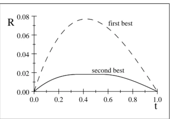
(12) [INSERT FIGURES 2a,b] The intuition behind Proposition 2 can be illustrated in this example. Figure 2.a shows the …rst best (dotted curve) and the second best path of the share of time spent to create knowledge (Figure 2.b shows the cumulated knowledge curves). The second best time spent to create knowledge is lower than the …rst best, because the employer does not receive 100% of the return of his “investment” in knowledge accumulation. Indeed, because of the hold-up problem, the employer has to share the returns of his investment in knowledge with the employee (the classical under-investment argument in hold-up models). The new feature is that the employer will permit an increase in the time spent to create knowledge during the employee’s mid-career. In the …nal phase of her career, the example shows that the …rst best and the second best allocations of time coincide. [INSERT FIGURE 2c] In this example, the outside option of the knowledge worker is given by: R (t) = (T. t) A K(t).. Now let us compare how the outside option evolves through time when the employer uses the …rst best path of working time allocation and when he uses the second best path (see Figure 2.c): The dotted curve (respectively, the continuous curve) represents the outside option of the knowledge worker when the employer uses the …rst best (respectively, second best) allocation of working time. In the second best situation, the …rm has to o¤er a cumulated wage that ful…ls condition (1). If it uses the …rst best path, it has to pay a RT total amount W (0) = w ( ) d ' 0:08 to the worker. According to Proposition 2, this is not optimal. If 0. instead the …rm uses the second best path, the outside option curve becomes ‡atter and it only has to pay less than 0:02 to the knowledge worker.. 3.2. Optimal wage pro…les. The empirical literature has shown that the Ben-Porath (1967) model matches age-earning pro…les (e.g. Heckman 1976 and Rosen 1976). The main feature of the empirical experience-earning pro…le is that the earning function is a hump-shaped function of experience. The following result shows that our model is compatible with this empirical evidence (we still consider that r = 0). Proposition 3 [Hump-shaped life cycle wage pro…le]: There always exists an optimal hump-shaped experience-earnings pro…le. The form of the optimal wage pro…le is constrained by the non-quitting constraint, i.e. the remaining earnings W (t) have to be greater than the outside option R (t) at any time t. In terms of the necessary 10.

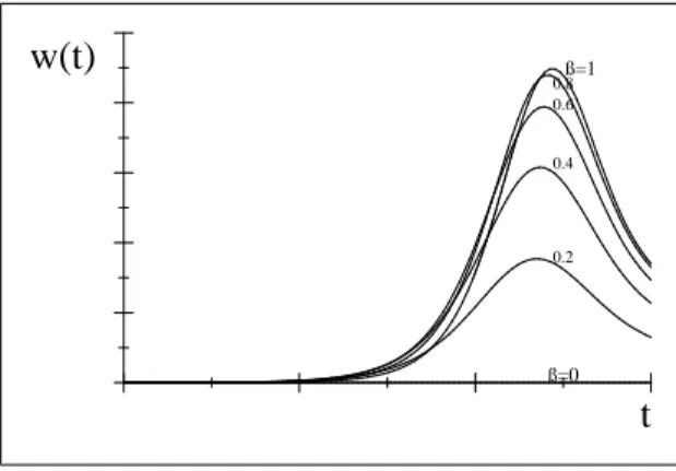
(13) conditions (8) and (9), the dynamics of the shadow price of knowledge remaining wages. and the shadow price of the. are linked through the opportunity cost of retaining the employee, which is represented. by '. The shadow price of the remaining earnings is non increasing, _ = w paid at time t0 rather than t with t. '. 0, because one unit of wage. t0 does not a¤ect W (t) but increases W (t0 ).. We know that the shadow price of the remaining wages is strictly positive,. > 0, over [0; tb ). Hence,. the employer has an incentive to postpone the earnings of the employee and then w (t) = 0 over [0; tb ). In the last phase [tb ; T ], the employer can spread the total earnings, W0 = W (tb ) = R (tb ), such that the non quitting constraint is ful…lled. There are then many optimal wage pro…les. The …rst polar wage pro…le is such that the employer o¤ers all the earnings W (tb ) at the end of the horizon and the second polar wage pro…le is such that the employer binds the non-quitting constraint at each time, i.e. W (t) = R (t) for all t 2 [tb ; T ].7 Then, the optimal wage pro…les are then such that the remaining earnings function is: W (t) = where s (t) 2 [0; 1]. Using w (t) =. R (tb ) for t 2 [0; tb ] s (t) R (tb ) + (1 s (t)) R (t) for t 2 [tb ; T ]. _ (t), we can deduce the optimal wage: W w (t) =. s_ (t) [R (tb ). 0 for t 2 [0; tb ] R (t)] (1 s (t)) R_ (t) for t 2 [tb ; T ]. Clearly, the function s(t) is not uniquely determined. In the proof of Proposition 3 we show that we can choose a sigmoid function s(t) such that the optimal wage pro…le is hump-shaped and Example 3 provides a numerical illustration. Figures 3.a and 3.b illustrate the result of Proposition 3. The non quitting constraint ZT states that the remaining earnings at any time t, W (t) w ( ) d , have to be larger than the optimal t. outside option R (t) = (T. t) ( K (t)). It is possible to …nd W such that it is larger than the optimal. outside option curve R (t). Example 3: As in Example 2, we specify the functions as follows:8 l. 1 2 2l .. (K) = AK with A > 0 and v (l) =. We also focus on the optimal solution such that k increases over only one interval [ta ; tb ]. We set. T = 1, K(0) = 0, A = 1=2, and. = 0:8.9 [INSERT FIGURES 3a,b]. Figures 3a and 3b display hump-shaped wage pro…les that resemble the bell curve of a normal distribution. This is because we use a sigmoid function s(t) and assume a low level of initial human capital. As example 3’(below) shows, it is possible to generate wage pro…les that look like those in the data, in particular, one w (t) = R_ (t) = ( K (t)) + (T t) 0 ( K (t)) k (t). resolution of the …rm’s problem under this speci…cation is relegated to Appendix B. 9 And the additional parameters are set to: = 1:2; = 8. See Appendix A for the parametric function used in this example (proof of Proposition 3). 7 Then 8 The. 11.

(14) that is concave everywhere, with the biggest increases in wages occuring at the beginning of a career, such as Figure 2 in Murphy and Welch (1990). Example 3’: We set s(t) = 0:2t + 0:8; r = 0; K(0) = 1; A = 1;and. = 0:8:. [INSERT FIGURE 3c]. 3.3. Enforceability and speci…city of knowledge. The most important parameter of our model is. and it can be interpreted in two di¤erent ways. First,. determines the degree of severity of the enforcement problem. Indeed, if. = 0, the employee has no incentives. to quit the …rm and the employer can then implement the …rst best path of knowledge accumulation without o¤ering any positive wage to the employee. If. > 0, the employer has to take into account the non-quitting. constraint and to distort the knowledge accumulation path. Second, 1 of knowledge ( = 0 being full speci…city and. measures the degree of speci…city. = 1 being full general knowledge). The latter interpretation. is in line with Becker (1962) who distinguishes two categories of human capital, speci…c and general human capital. Speci…c human capital is related to a speci…c …rm’s products or services, whereas general human capital can be used in a large range of di¤erent …rms. More speci…cally, we study the e¤ect of a change in many optimal wage pro…les, we analyse the e¤ect of. on the outcomes of the model. Since there exist on the optimal total earnings, W0 , rather than on. the whole wage pro…le, w (t). We then study the e¤ect of. on the outcomes (k (t) ; K (t) ; W0 ) and also. on the length of the phase [ta ; tb ]. We concentrate on the following speci…cation of the general model: we assume, as in examples 1, 2 and 3 that the pro…t generated by knowledge inside the …rm is proportional to the accumulated amount of knowledge, v (l) = l. 1 2 2l .. (K) = AK. The value of the routine task is speci…ed as. Using this speci…cation and focusing on the solution with only one phase where k increases. (again see Appendix C for su¢ ciency), we can show the following result: Proposition 4 [Enforceability and speci…city of knowledge]: As the severity of the enforcement problem decreases and/or knowledge becomes more speci…c (. decreases):. (i) The phase of increasing fraction of time devoted to the knowledge task becomes shorter. Formally, jtb. ta j decreases when. decreases.. (ii) Both the fraction of time devoted to the knowledge task and the total amount of knowledge accumulated at any time increase. Formally, both k (t) and K (t) increase when. decreases, for all t 2 [0; T ].. (iii) The change in the total wage of the knowledge worker, W0 , is ambiguous. The …rst two results (i) and (ii) are quite intuitive. When knowledge becomes more …rm-speci…c, the value of the outside option of the knowledge worker becomes smaller and it becomes easier to retain her, i.e. the situation is closer to the …rst best situation. Then the duration of the phase where k increases becomes. 12.

(15) smaller. (Note that there is no such phase in the …rst best case, which is incentive compatible in the situation where. = 0). The total amount of knowledge accumulated over the whole horizon also increases. When. decreases, the severity of the hold-up problem is reduced, the "investment" k (and so K) then increases and becomes closer to the …rst best path (see Figures 4.a and 4.b for a numerical illustration). The result reported in point (iii) can be explained as follows. An increase in the speci…city of knowledge has two e¤ects on the outside option, which work in opposite directions. On the one hand, the more speci…c the knowledge, the lower the value of the outside option of the knowledge worker, and this allows the employer to o¤er her a lower total wage. On the other hand, when knowledge becomes more speci…c, the employer can a¤ord to leave her more time to accumulate knowledge. Hence, the amount of accumulated knowledge is larger, which in turn increases the knowledge worker’s outside option. These two opposite e¤ects explain the ambiguous impact of knowledge speci…city on the worker’s wage. The following example illustrates these results. Example 4: As in example 2, we set T = 1 and A = 1=2. Using the parametric hump-shaped wage pro…le used to plot Figure 3.a, Figure 4.c illustrates this optimal wage pro…le for various values of . We can see that when The larger. is, the greater the cumulated wage (the greater the area below the wage pro…le curve). Notice. that the wage pro…le for (R (t). changes, the optimal wage pro…le is a¤ected.. = 0 is w (t) = 0 for all t 2 [0; T ], because the worker has no outside option. 0).. [FIGURES 4a,b,c]. 4. Extensions: initial knowledge level, discounting, and concave utility. 4.1. Role of initial knowledge level. The seminal contribution of Mincer (1974) has initiated many empirical works regarding the returns to schooling (see Heckman et al. 2003 and Belzil 2007 for surveys of the literature). More recently, Hugget et al. (2011) have shown that di¤erences in lifetime earnings are mainly due to initial conditions. In this section, we show how a change in the initial knowledge level (K0. K (0)) a¤ects our main results.. We concentrate on our main example. The pro…t function is linear, speci…city is denoted 1. (K) = AK. The degree of knowledge. 2 (0; 1). The value of the routine task is speci…ed as v (l) = l. 1 2 2l .. Using this. speci…cation and focusing on the solution with only one phase where k increases (again see Appendix C for su¢ ciency), we can show the following result:. 13.

(16) Proposition 5 [Initial knowledge level]: As the initial stock of knowledge K0 increases, (i) The fraction of time devoted to the knowledge task is shifted downwards in the …rst phase, then upwards in the second phase, and is not a¤ ected in the third phase. Formally, when K0 increases, k (t) becomes greater for each t in [0; ta ], smaller for each t in [ta ; tb ], and is not a¤ ected over [tb ; T ]. (ii) The cumulated knowledge always increases. Formally, K (t) becomes greater at each t when K0 increases. (iii) The phase of increasing fraction of time devoted to the knowledge task becomes longer. Formally, jtb. ta j increases when K0 increases. However, both ta and tb decrease when K0 increases. (iv) The total earnings are greater and the phase where the wage pro…le is ‡at is shorter. Formally, W0. increases when K0 increases. Moreover, w (t) = 0 over [0; tb ] and tb decreases when K0 increases. When the initial knowledge of the employee increases, her outside option, R (t) = (T greater and reaches its falling stage at an earlier time. A larger K0 leads to a larger. t) ( K (t)), is. ( K (t)), and then tb. is smaller (see Figure 5.a). The employer has an incentive to reduce the share of time devoted to knowledge creation at the beginning in order to limit the increase of the outside option of the employee. On the other hand, the switching time at which this share is allowed to rise occurs quite early because the outside option of the agent decreases quickly (see Figures 5.b and 5.c). The following example illustrates the results. Example 5: We set T = 1, A = 1=2 and. = 0:8.. Using the parametric hump-shaped wage pro…le used to plot Figure 3.a, Figure 5.d illustrates the optimal wage pro…le for various values of K0 . [INSERT FIGURES 5a,b,c,d]. 4.2. Role of discounting. To show our main result, we have made the simplifying assumption that both the employer and the employee do not discount future earnings. In this section, we relax this assumption and consider the case where both the employer and the employee discount future earnings at a positive rate r. The problem to be solved by the employer can then be written as follows:. max. k( )2[0;1]; 0 w( ). Z. T. e. r. [ (K( )) + v(1. 0. subject to _ ) = k( ); K( K(0) = 0 (…xed),. 14. k( )). w ( )] d.

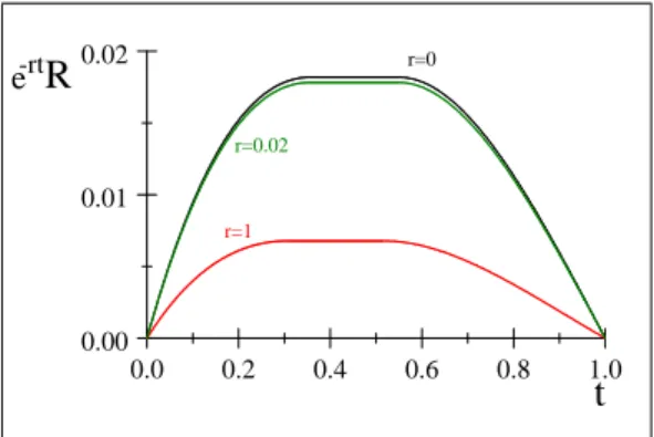
(17) and the non-quitting constraint: Z. T. e. r(. t). w( )d. ( K (t)). t. Z. T. e. r(. t. t). d for all t 2 [0; T ] .. It is convenient to rewrite the non-quitting constraint as follows: Z (t). e. rt. R (t) for all t 2 [0; T ] ;. RT r where Z (t) e w ( ) d is the sum of present value wages to be paid after time t, and e t RT r e ( K (t))d is the present value of the outside option for an employee if she quits at t. t. rt. R (t). The following proposition shows how our main result is a¤ected when the discount rate is positive:. Proposition 6 [optimal time allocation, r > 0]: When the employer and the employee share the same discount rate r > 0,. (K) = AK and v (l) = l. 1 2 2l ,. the second best solution has the following properties.. If k (t) > 0 over [0; T ): (i) There exists at least one time interval (t0 ; t00 ) over which k( ) is increasing, i.e. the employer promises a phase of acceleration of human capital accumulation in order to induce the employee to stay longer. (ii) There exists tb < T , such that over the interval [tb ; T ], k(t) will be falling (k_ < 0). (iii) There exists ta. 0, such that over the interval [0; ta ], k(t) will be falling (k_ < 0).. (iv) The necessary conditions are su¢ cient. This proposition shows that our results are not qualitatively a¤ected by a change in the discount rate. The following numerical example illustrates this point. Example 6: We set T = 1, A = 1=2 and. = 0:8.. [INSERT FIGURES 6a,b,c,d] Figure 6.a represents the present value of the outside option e. rt. R (t) for di¤erent values of the discount. rate (for a realistic value of 2% and for a very large value of 100%). As in the case without discounting, the outside option increases (in present value), then reaches a plateau and …nally decreases. Figures 6.b and 6.c illustrate the share of time devoted to knowledge accumulation and the cumulated knowledge, respectively. There is no qualitative di¤erence when the discount rate varies (r = 0; r = 0:02, r = 1). For a discount rate of 2%, the curve of the share of time devoted to knowledge accumulation is slightly above the corresponding curve in the case of no discounting. Similarly, the curve of cumulated knowledge, K; is only slightly a¤ected by an increase in the discount rate from 0% to 2%. Using the parametric hump-shaped wage pro…le used to plot Figure 3.a, Figure 6.d represents this optimal wage pro…le for various values of r.10 1 0 One may wish to introduce an exogenous (Poisson) quit process with arrival rate q > 0 into the model. It turns out that this additional feature interacts with the discount rate r in a non-trivial way. Quitting probability introduces a non-trivial distortion (because of the non-quitting constraint).. 15.

(18) 4.3. Concave utility. Up to this point, we have considered that the employee’s utility function is linear, i.e. that the utility derived from wage w (t) is exactly w (t). Let us relax this assumption and consider the case of a concave utility function u (w), with u (0) = 0, u0 (w) > 0 and u00. 0 for all w. 0. Let U (t) be a new state variable. denoting, for the "promised utility" (as in Spear and Srivastava 1987) starting at t, whether the employee stays with the …rm until the time horizon T :. U (t) =. ZT. u (w ( )) d :. t. This "promised utility" must exceed what the employee can achieve if she quits at t, U (t). R (t). Since the wage cannot be negative, w ( ). (T. t) u ( ( K (t))) :. 0, we have U_ (t) =. u (w ( )). 0:. The employer’s optimization programme is to choose the time path k (t) and w (t) in order to maximize the following expression (we consider the case where r = 0 and K0 = 0): max. k( )2[0;1]; 0 w( ). Z. T. [ (K( )) + v(1. k( )). w ( )] d. 0. subject to the non quitting constraint: U (t). R (t). (T. t) u ( ( K (t))) for all t 2 [0; T ] ;. (14). and, K_ (t) = k (t) ; 0 U_ (t) =. k (t). 1; w (t). 0;. u (w ( )) :. Note that K0 = 0 is given and K (T ) is free. The following proposition shows how our main result is a¤ected when the utility is concave (for simplicity, we assume an Inada condition, v 0 (1) = 0).11 Proposition 7 [Concave utility, u (w)]: Assume that the employee has a (strictly) concave utility function, u (0) = 0, u0 > 0 and u00 < 0. If k (t) is interior over [0; T ), there exists at least one time interval (t0 ; t00 ) over which k( ) is increasing, i.e. the employer promises a phase of acceleration of human capital accumulation in order to induce the agent to stay longer. 1 1 It can be shown that the wage pro…le is not unique even when u(w) is strictly concave. This is because u(w) appears indirectly in an integral constraint, and does not appear directly in the objective function.. 16.

(19) 5. Link with empirical evidence. Our theoretical results are broadly consistent with the empirical evidence on life-cycle human capital accumulation, and wage pro…les. Human capital accumulation being di¢ cult to measure, the empirical literature provides mainly documentation of formal on-the-job training. The evidence is consistent with our result that human capital accumulation is not concentrated at the beginning of the career.12 Indeed, Loewenstein and Spletzer (1997) show that delayed formal training is frequent.13 More precisely, they show that, for a given job duration, more workers receive training in year t + 1 than in year t (see Loewenstein and Spletzer 1997, Table 3). This is consistent with our result that k may be increasing, k being interpreted as the probability for a worker to receive training at time t. This is not the case in Ben-Porath’s model. Concerning life-cycle wage pro…les, we have shown in subsection 3.2 that our theory can produce a humpshaped wage pro…le, in line with Heckman (1976) and Rosen (1976). In particular, a strictly concave wage pro…le, with the biggest increase in wages occuring at the beginning of a career, as in Fig. 2 in Murphy and Welch (1990), is consistent with our model when K(0) is su¢ ciently high.. 6. Discussion and related literature. As already mentioned, our paper contributes to the literature on the accumulation of human capital within an organizational context. Other papers have considered the human capital accumulation problem within an organization. Smid and Volkerink (1999) extend the analysis of speci…c schooling by Hashimoto (1981) by introducing non-speci…c or general schooling within a two-period framework. In the …rst period, the employer and the employee not only have to choose the level of investment in human capital and the division of costs and bene…ts, but also have to decide on the speci…city of the training. In the second period, (private) information on the productivity of schooling becomes available, and the employee may decide to quit, or the employer may dismiss the employee. They analyze the consequences of subsidies or taxes on schooling. The degree of speci…city of training is also an important feature of our paper. However, we consider the speci…city of knowledge as an exogenous parameter and analyse its in‡uence on knowledge accumulation and on the 1 2 Bartel (1995) …nds that 47% of the individuals hired before 1980 have received some formal training by 1990. This empirical result suggests that human capital investments are not only undertaken at the beginning of a career. 1 3 They present several lines of evidence. They …rst show that the probability of job separation is negatively correlated with tenure (using the 1988-1991 National Longitudinal Survey of Youth, NLSY). Then, they focus on the timing of training. They show that the relationship between tenure and the probability of having ever received training is positive (using the 1991 supplement to the Current Population Survey, CSP). They argue that there are several interpretations of this result: either training increases with tenure or those workers who form good matches both receive training and stay longer within …rms, whereas bad matches do not receive training and are more likely to terminate. They …nally show that, among groups of workers who change jobs after the same number of years, more workers receive training in year t+1 than in year t. They argue that the simple human capital model predicts that training will occur as soon as possible, and that delay in training may be due to delay in the revelation of information about the quality of employer-employee match. Our model is an alternative explanation for this evidence.. 17.

(20) life-time earning of the knowledge worker. As in the present paper, Azariadis (1987) and Bernhard and Timmis (1990) consider models of human capital accumulation problems with contracting. Azariadis (1987) considers implicit contracts as devices for redistributing returns to human capital over time when workers cannot borrow (in an overlapping generation model). He provides a condition for self-enforcing contracts to exist, and explores how existence depends on the rate of interest and on human capital speci…city. Bernhard and Timmis (1990) focus on the implications of capital market imperfections for the form of long term wage contracts. As in Azariadis (1987), …rms can mediate …nancially for workers to reallocate returns to human capital over time. Workers can smooth their consumption over time, and human capital accumulates according to an exogenous process. Di¤erently, the present paper focuses on endogenous human capital accumulation. Our paper contributes to the literature on the hold-up problem14 by exploring a trade-o¤ that has not been analysed previously. On the one hand, by letting the knowledge worker accumulate knowledge early, the employer obtains large returns on this investment as long as the worker stays with the …rm, but the incentives for the worker to quit become stronger over time until she approaches her retirement age. On the other hand, letting the worker accumulate knowledge later, the employer obtains lower returns because the remaining horizon is shorter, but the worker’s incentives to quit become weaker. Hvide and Kristiansen (2012) also deal with the management of knowledge workers. They study how both …rm-speci…c complementary assets and intellectual property rights a¤ect the management of knowledge workers. They focus on the trade-o¤ between moral hazard and hold-up. Our model is related to dynamic models of hold-up. Guriev and Kvasov (2005) show that, if contracts are allowed to extend beyond the breakup of relationship, e¢ ciency can then be achieved by a sequence of constantly renegotiated …xed term contracts, or by a perpetual contract that allows unilateral termination with advanced notice. In our model, after the breakup the employer is allowed only limited compensation, and therefore e¢ ciency is not achieved. In Pitchford and Snyder (2004) the seller can make gradual investment installments, and the buyer has an incentive to pay after each installment, so the hold-up problem can be mitigated if there is no known, …nite end to the number of installments. In our model, there is a …nite end to the installments because the time horizon is …nite. Furthermore, installment payments are not possible because the employee cannot borrow, and does not have adequate income to post a bond during training.15 Che and Sakovics (2004) consider the role of anticipated future investments in a joint project. Two 1 4 The hold-up problem is a crucial factor in the determination of the evolution of a bilateral relationship when agents make, ex ante, sunk and speci…c investments which will increase, ex post, the surplus of the relationship. Then, being unable, ex ante, to secure a share of the surplus in relation to the amount of their sunk investments, later agents will have to negotiate the division of the surplus, taking account that their bargaining power will have changed. This is "the fundamental transformation" (Williamson, 1979), the value of their speci…c investments being di¤erent "out of the relationship" than "within". 1 5 Various remedies have been proposed as safeguards against holdup, ranging from vertical integration (Klein et al. 1978, Williamson 1979), property rights allocation (Grossman and Hart, 1986, Hart and Moore, 1990), contracting on renegotiation rights (Chung, 1991, Aghion et al., 1994), option contracts (Nöldeke and Schmidt, 1995, 1998), production contracts (Edlin and Reichelstein, 1996), relational contracts (Baker et al. 2002), …nancial rights allocation (Aghion and Bolton,1992, Dewatripont and Tirole, 1994, and Dewatripont et al. 2003) and hierarchical authority (Aghion and Tirole 1997) to injecting market competition (MacLeod and Malcomson 1993, Acemoglu and Shimer 1999, Felli and Roberts 2011, and Che and Gale 2003).. 18.

(21) partners make investments and negotiate to share the surplus within an in…nite horizon setting. Players receive payments only when an agreement is reached (and the game ends). Their main result is that for su¢ ciently patient players, the hold-up problem may be alleviated because of the shadow of the future. Smirnov and Wait (2004) focus on the timing of investments in a bilateral relationship where (i) two players can invest only once, and (ii) trade occurs only once and only if both players have made a speci…c investment. Their paper shows that if the potential investment horizon is continually extended, players move in alternation from a prisoners’dilemma to a coordination game. Our model is very di¤erent from those of Che and Sakovics (2004) and Smirnov and Wait (2004) as we study a situation where players get payments all along the game. Compte and Jehiel (2003) study the e¤ect of the outside option (the value of which changes over time, depending on the history of o¤ers and concessions) on the equilibrium of a bargaining game. They consider a complete information game that has two features. First, at any point of time, each party has the option to terminate the game (in contrast to our model, where only one party, namely the employee, has this option). Second, in case of termination, the payo¤s are assumed to depend on the history of o¤ers or concessions made in the bargaining process. They show that for a large class of such games, gradualism is a necessary feature. They also derive an upper bound on concessions. Finally, even though our model’s main focus is on how the time path of human capital accumulation is distorted because of incomplete contracts, it is also potentially useful for thinking about the “exploration and exploitation” relationship which has been discussed in the management literature where adaptive processes balance between the exploration of new possibilities and the exploitation of old certainties (Schumpeter 1934, Holland 1975). According to March (1991), “exploration includes things captured by terms such as search, variation, risk taking, experimentation, play, ‡exibility, discovery, innovation”, while exploitation “includes such things as re…nement, choice, production, e¢ ciency, selection, implementation, execution”. As noted by Ben Porath (1967), the pioneering work of Becker (1962, 1964) emphasized the demand side of human capital formation. Thus, Becker’s focus is on the exploitation motive. Ben Porath (1967) emphasizes the supply side, the investment costs. This re‡ects the exploration motive. In our paper we consider the two interrelated motives within an organization where the value of the outside option evolves endogenously. Our non-monotonicity result, which shows that the rate of change in knowledge comes in sudden bursts, may be viewed in the light of the theory of punctuated dynamics (Eldredge and Gould 1972), according to which evolution is not a gradual process. Periods of exploration where things change drastically are inserted between prolonged periods of exploitation where only minor changes take place.. 7. Conclusion. In this paper, we have considered a knowledge accumulation problem within an organization. We have shown how the employer optimally distorts the knowledge accumulation path and chooses a wage pro…le in. 19.

(22) order to mitigate the opportunism problem. We have shown that knowledge accumulation is delayed. The fraction of working time allocated to knowledge creation is highest at the early career stage, falls gradually, then rises again, before falling …nally toward zero. We have also shown that an increase in the severity of the enforcement problem (or a decrease in the degree of …rm-speci…city of knowledge) decreases the share of working time allocated to knowledge creation, and decreases cumulated knowledge. Moreover, such an increase can increase or decrease the life-time income of the knowledge worker. Our main result is robust to an increase in the initial knowledge level, to a change in the discount rate, and to a change in the worker’s utility function. Our model …ts well with existing empirical evidence. Our main result, the non-monotonicity of investment in human capital, …ts well with the reported evidence that delayed formal training (i.e. an increasing quantity of formal training over time) is frequent. Our model matches also the main feature of age-earning pro…les, that the optimal experience-earning pro…le is a hump-shaped function of experience (among other solutions). And, consistently with recent evidence that di¤erences in lifetime earnings are mainly due to initial conditions, we have found that an increase in the initial knowledge level has a positive e¤ect on earnings.. Appendix A: Proofs Proof of Proposition 1: Since b (K) <. (K), the value of knowledge is larger when the employee stays. with the …rm, the optimal quitting time is t = T . The joint surplus maximization problem reduces to max k. ZT. e. r. [ (K ( )) + v (1. k ( ))] d ;. 0. where 0 Let 1. k. k( ). _ ) = k( ). 1 and K(. be the co-state variable,. and. be the multipliers associated with the constraint k. 0 and. 0. Write the Lagrangian L=e. r. (K) + e. r. v (1. k) + k + k + (1. k). The necessary conditions are @L = @k 0;. k. e 0;. r. v 0 (1 1. k) + k. + k = 0;. _ = @L = e @K. r. 0. =0 (1. (15) k) = 0. (K). (16) (17). and the transversality condition is (T ) = 0 Integration of (17) gives. RT (t)] = t 0 (K ( )) e r d . It follows that Z T 0 (t) = (K ( )) e r d > 0 for all t < T. (18). [ (T ). t. 20. (19).

(23) Using (17), we have _ =. e. 0. r. (K) < 0:. (20). Assuming an interior solution, we have (t) = (t) = 0, and using (15), we have RT using (19), we have v 0 (1 k) = t 0 (K ( )) e r( t) d . Di¤erentiating, we obtain: k_ =. To show that k_ < 0 we must prove that p_ = rp. 0. 0. [. 0. =e. r. v 0 (1. k); and. rv 0 ] : k). (K). v 00 (1. > rv 0 . De…ne the current-value shadow price p = ert. and p(T ) = 0. Along the optimal path, rp cannot exceed 0. From its de…nition, p = v for all t 2 (0; T ). Therefore. 0. (K). 0. 0; then. (if it does, then p cannot go to zero).. rv > 0. Thus k_ < 0. 0. Proof of Proposition 2: Let us show (i), (ii), and (iii). Let us …rst show that k_ (t) > 0 when ' (t) > 0 and k_ (t) < 0 when ' (t) = 0. Assume that ' (t) > 0 for all t 2 (t0 ; t00 ). Using (7), we have W (t) = R (t) for all t 2 (t0 ; t00 ), or, ZT. w ( ) d = (T. t) ( K (t)) :. t. Di¤erentiating this condition, we …nd: w (t) =. ( K (t)) + (T. t). 0. ( K (t)) k (t) :. Using ' (t) > 0 and (9) we have _ < 0. Using (5) and (6), we obtain =. (21). =. 0. Since _ < 0, we have. > 0 for all t 2 (t0 ; t00 ) and then w (t) = 0. Hence, di¤erentiating (21) and rearranging we …nd: 2 k_ (t) =. 0. ( K) k + (T (T t). t) ( 00 ( K)) k 2 > 0: 0 ( K). (22). Now assume that ' (t) = 0 for all t 2 [t1 ; t2 ]. Using (8) and di¤erentiating (4), we have v 00 (1. 0. (K) = _ =. _ or, k)k,. k_ = Let us look for solution such that Using (4), we have. = v 0 (1. and. 0. (K) < 0: k). (23). v 00 (1. are continuous.. k) > 0 and di¤erentiating, we have _ =. v 00 (1. _ Since k)k.. (T ) = 0,. there exists an interval [tb ; T ] such that _ (t) < 0 and then k_ (t) < 0 for all t 2 [tb ; T ].. Assume that there exists t1 > 0 such that k_ (t) > 0 for all t 2 [0; t1 ]. Hence, we know from the reasoning. above that 0=. w (0) = T. 0. (0) k (0) ;. and then k (0) = 0. But we have assumed that k (t) > 0 for all t 2 [0; T ). Hence there exists ta > 0 such that k_ (t) < 0 for all t 2 [0; ta ].. Now assume that there is no phase k_ (t) > 0, i.e. we have ' (t) = 0 = _ (t) for all t. Since (0) = 1, we. must have (t) = 1 for all t. Using (5), we have. (t) = (t) = 1 > 0. Hence w (t) = 0 for all t and then 21.

(24) W (t) = 0 for all t. Using (7), we have 0 = W (t). R (t) and then R (t) = (T. t) ( K (t)) = 0 for all t,. i.e. K (t) = 0 for all t. But we have assumed that k (t) > 0 for all t 2 [0; T ). See Appendix C for a proof of (iv). Proof of Proposition 3: Notice that R_ (tb ) = 0, R_ (t). • (t) 0. Moreover, we have R. 0 over [tb ; T ].. Indeed, • (t) = R. 2. 0. ( K ) k + (T. t). 2 00. 2. ( K ) (k ) + (T. 0. t). ( K )k_ :. • (t) < 0 over (tb ; T ). Since k_ < 0 for t 2 (tb ; T ), we have R We are looking for w (:) that satis…es the necessary conditions. The …rst condition is the non quitting constraint:. W (t). ZT. w( )d. R (t) = (T. t) ( K (t)) ;. (24). t. The second condition ensures that the principal leaves minimal rents to the agent: W (tb ) = R (tb ) and W (T ) = R (T ) = 0. (25). In order that the wage pro…le …ts with the evidence, we want to …nd a hump-shaped wage pro…le, i.e. we require that: w_ (T ) < 0. w_ (tb ). (26). 0 for all t:. (27). We also need that the wage is non negative: w (t) Let us de…ne the following function: W (t) =. R (tb ) for t 2 [0; tb ] ; s (t) R (tb ) + (1 s (t)) R (t) for t 2 [tb ; T ]. (28). where s (t) for all t 2 [0; T ]. Remark that condition (24) holds because R increases over [0; ta ], reaches a plateau over [ta ; tb ], and decreases over [tb ; T ]. Condition (25) also holds only if s (T ) = 0: Using w =. (29). _ (by de…nition of W ), condition (27) is equivalent to: W _ (t) = s_ (t) (R (tb ) W. for t 2 [tb ; T ]. Using w_ =. R (t)) + (1. s (t)) R_ (t). 0. (30). • , condition (26) can be rewritten as follows: W • (tb ) W. • (T ) : 0<W 22. (31).

(25) Since • (t) = s• (t) (R (tb ) W. 2s_ (t) R_ (t) + (1. R (t)). • (t) ; s (t)) R. condition (31) can be rewritten as: • (tb ) = W. 2s_ (tb ) R_ (tb ) + (1. • (tb ) < 0; s (tb )) R. (32). and, using (29): • (T ) = s• (T ) (R (tb ) W • (tb ) Since R_ (tb ) = 0 and R. • (T ) > 0 2s_ (T ) R_ (T ) + R. R (T )). (33). 0; (32) always holds.. Hence, we have to …nd s () such that (29), (30) and (33) hold and s (t) 2 [0; 1] for all t in [tb ; T ]. Let us consider the following function:. s (t) = where. > 0 and. (34) !. • (T ) 2 R_ (T ) R + 2 R (tb ). B= where. (T t) e B(t T ) ; 1 + (T t) e B(t T ). ;. (35). > 1.. First, notice that (29) holds, i.e. s (T ) = 0. Second, (30) holds because we know that R_ (t) R (tb ). 0 and. R (t) and eB(T. s_ (t) =. t). (T. (B (T t) eB(T. t) + 1) t). +1. 2. < 0.. (36). Third, using eB(T. t). 2. (B (T. (T and, s_ (T ) =. and s• (T ) = 2 (B. t) + 1) eB(T. t)) + 2 (B (T. s• (t) =. t) eB(T. t). +1. t). 2B. B 2 (T. t) ;. 3. ). Condition (33) writes:. • (T ) = 2 (B W. ) (R (tb ). • (T ) > 0; R (T )) + 2 R_ (T ) + R. or, B> which is true because. • (T ) 2 R_ (T ) R + ; 2 (R (tb ) R (T )). > 1 in (35).. Proof of Proposition 4: We …rst show point (i). We know from appendix B (taking K0 = 0) that ta and tb are the solution of = (T T. 3. tb ) ta. =. ln. T T. tb ta. 1 (T ta ) (ta ) 2 (T 2ta ) 23. 2 + 3. 1. T T. tb ta. 3. !. (37). 2. (38).

(26) 2. Multiplying both sides of (38) by 1= (T. ta ) , we have:. T T. 3. tb ta. =. 2. 1 2 (T. (ta ) 2ta ) (T. ta ). Plugging this condition into (37), we obtain: =. 1 ln 3. 2. 1 2 (T. (ta ) 2ta ) (T. ta ). !. 2 + 3. 1 2 (T. 1. 2. (ta ) 2ta ) (T. ta ). !. :. This condition characterizes ta as a function of . Di¤erentiating this condition with respect to , we have: dta = d The function ta 7! 2. (ta ) (T. 2 2 1 (ta ) (T ta ) 2 (T 2ta ). 2. 3ta (T (T. 2ta ) (T. 2. 2. ta ) (T ta ) + (ta ). 2ta ) 2. (2T. < 0: 3ta ) T. increases with respect to ta . Indeed, the derivative of the function ta 7!. ta ) is given by ta 7! 4ta (T. ta ). T 2. ta > 0. Using (38), we have that tb decreases when ta. increases. Hence, tb increases with respect to . Now consider point (ii). We know from the examples that the optimal cumulated knowledge is given by 8 (T tb )3 > A (T + Ata A 2t t if t 2 [0; ta ] < ta )2 3 K (t) = ; (39) A (TT tbt) if t 2 [ta ; tb ] > : 2 1 2 1 2 A (T tb ) + A (t tb ) T 2 t + 2 tb if t 2 [tb ; T ]. and then,. 8 > <. dK (t) = > d :. 3 A(T (T. tb )2 dtb ta ) 2 d. tb )3 a t < 0 if + A dt d ta )3 2 1 dtb 3A (T tb ) T t d < 0 if t 2 [ta ; tb ] b 2A (T tb ) dt d < 0 if t 2 [tb ; T ]. + 2 A(T (T. The optimal share of time devoted to knowledge accumulation is given by 8 (T t )3 > < A (T tab )2 + Ata At for t 2 [0; ta ] ; 3 2 k (t) = A (T tb ) (T t) for t 2 [ta ; tb ] ; > : A (T t) for t 2 [tb ; T ] , and then. 8 > <. dk (t) = > d :. 3 A(T (T. :. (40). tb )3 a + A dt d < 0 for t 2 [0; ta ] ; ta )3 2 b t) dt d < 0 for t 2 [ta ; tb ] ;. tb )2 dtb ta ) 2 d. + 2 A(T (T. A (T. tb ) (T 0 for t 2 [tb ; T ] ,. 2. t 2 [0; ta ]. Now consider point (iii). Using (39) for t = T , the total amount of accumulated knowledge is given by K (T ) = 32 A (T. 2. tb ) . Hence K (T ) decreases with respect to .. We also have W0 = R (tb ) = (T. tb ) AK(tb ) = A2 (T. 3. tb ) .. Proof of Proposition 5: We …rst prove points (i), (ii) and (iv). We can easily show that the derivative of k with respect to K0 is 8 dta > 3 2 A d(tb ta ) + A (1 ) 1+ 2 2 dK < 0 for t 2 [0; ta ] ; dK0 0 dk (t) < 2 2 dtb = A (T tb ) (T t) d > 0 for t 2 [ta ; tb ] ; > dK0 : 0 for t 2 [t ; T ] , b. 24.

(27) and the derivative of the cumulative knowledge is (using the fact that does not depend on K0 ): 8 3 dta > 1+A 1 dK0 t > 0 if t 2 [0; ta ] dK (t) < 2 1 dtb = 3A (T tb ) T t dK0 > 0 if t 2 [ta ; tb ] > dK0 dtb : 2A (T tb ) dK > 0 if t 2 [tb ; T ] 0 tb ) K (tb ) = A2 (T. The total wage is given by W0 = R (tb ) = A (T. 3. tb ) , and then, its derivative with. respect to K0 is dW0 = dK0. 3A2 (T. 2. tb ). dtb > 0: dK0. We now prove point (iii). From appendix B, we have: 2. 3. A and. =. (41). 2 1 3. (42). 2 (0; 1) is the solution of =. with. 2K0 + A (ta ) ; 2 (T 2ta ) (T ta ). =. ln ( ) +. 3. ;. T tb T ta .. Using (42) reveals that. does not depend on K0 . Using (41) and the fact that ta 7!. an increasing function, we deduce that an increase of K0 leads to an decrease of ta . Since by the increase of K0 , tb also decreases as K0 increases (and then we have tb. ta =. 1. (T. tb ) and then tb. dtb dK0. =. dta dK0 ).. 2K0 +A(ta )2 2(T 2ta )(T ta ). is. is not a¤ected. Also, since. =. T tb T ta ,. ta increases when K0 increases.. Proof of Proposition 6: The …rm o¤ers to the employee a package deal whereby it pays her a sum w ( ) at time , provided that she stays with the …rm until time to a prescribed time allocation scheme (k( ); 1 to knowledge creation, and 1. for all. 2 [0; T ], and works for the …rm according. k( )) where k( ) is the fraction of the workday to be spent. k( ) is the fraction of the day to be spent on other tasks. If the employee. quits at any time t < T , her full income stream from time t to T will be Z T R(t) = e r( t) ( K(t))d = ( K(t))ert (t). (43). t. where (t). e. rt. e r. rT. . Remark that, as r ! 0, the RHS goes to (T. The employee will stay with the …rm until T if and only if Vw (t). t) ( K(t)). R(t) for all t 2 [0; T ]. Thus, the …rm’s. package deal must satisfy the non-quitting constraint Z T e r( t) w ( ) d ( K(t))ert (t) for all t 2 [0; T ] , t. or,. Z. T. e. r. w( )d. ( K(t)) (t) for all t 2 [0; T ] .. t. Let us de…ne the remaining wage (discounted from 0) as a new state variable Z (t): Z t Z (t) Z0 z( )d for all t 2 [0; T ] , 0. 25. (44). (45).

(28) where Z0 is the present value of all future wage payments, and z is the discounted wage: z (t). e. rt. w (t). for all t 2 [0; T ]. The non-quitting constraint (44) can then be rewritten as: Z (t). ( K(t)) (t) for all t 2 [0; T ] ,. and the dynamics of Z is given by Z_ (t) =. (46). z (t) for all t 2 [0; T ].. The …rm must now choose the time path of the control variables k(t) and z(t) to maximize the objective function Vf. =. Z. T. e. r. [ (K( )) + v(1. k( )). e. r. [ (K( )) + v(1. k( ))] d. w( )] d. 0. =. Z. T. Z0 ;. (47). 0. subject to K_. = k. K(0). =. Z_ = 0. 0. (48). z. k(t) z(t). 1; 0:. and the non quitting constraint, using (43) and (46), Z (t). rt. R(t)e. ( K(t)) (t). (49). Note that Z0 must be chosen, which implies a cost, as seen in (47). There are no explicit restrictions on K(T ) and Z(T ). Necessary conditions: Let. (t) and (t) be the co-state variables associated with the state variables. K(t) and Z(t) respectively. Let (t), (t); constraints k(t). 0, 1. k(t). 0; z(t). (t) and '(t) be the multipliers associated with the inequality. 0 and Z (t). R(t)e. rt. = ( K(t)) (t). De…ne the Hamiltonian H. and the Lagrangian $ as follows H=e. rt. (K) + e. $ = H + k + [1. rt. v(1. k) + k. k] + z + ' Z. z (t) ; Re. rt. :. The necessary conditions include @$ = @k. e. rt 0. v (1. k) +. 26. +. = 0;. (50).

(29) @$ = @z 0;. 0, k. 0, z '. +. 0, k = 0, 0, Z. R. = 0; 0, 1. 0, ' Z. _ = @$ = e @K. rt 0. (51) k. Re. (K). '(. 0, (1 rt. k) = 0; z = 0. (52). =0. (t). 0. (53). ). (54). @$ =' @Z. _=. (55). The following transversality conditions are also necessary. Since Z0 is to be chosen optimally, at a cost, and there are no restrictions on K(T ) and Z(T ), we have (T ) = 0. (0). =. 1. (56). , (Z (0). 0 and Z (0). R (0)) = 0; R (0). (57). 0;. (T ) = 0.. (58). We look at a solution such that k is interior and the total wage Z (0) > 0. i h rT = 0 (from (48)), and (57), we have = 0 and then Using R (0) = A K(0) 1 er (0) = 1 Using our speci…cation of. (59) 1 2 2l ,. (K) = AK, v (l) = l. conditions (50), (51), (54) and (55) can be. rewritten as follows: =e. rt. k;. (60). =. 0;. (61). _ =A '. e. _= From (59), (58) and (63),. Z. rt. ;. (62). ':. (63). T. '(t)dt = 1:. (64). 0. This implies that there exists some interval [ta ; tb ] in which the constraint Z(t) Remark: Also, notice that if we write S(t) We also have S_ = A. e. rt. is continuous and. (t) = 0 for t 2 (tb ; T ]. We then have. rt. R(t) is binding.. R(t), then S(t) = A K(t) (t) and S (0) = S (T ) = 0.. _ _ )= k + K _ . Thus S(0) = A k (0) (0) > 0 > S(T. Let us …nd a solution such that. e. rT. .. (t) = 1 for t 2 [0; ta ); _ (t) < 0 for t 2 [ta ; tb ] and. (t) > 0 for t 2 [0; tb ). 27. A K (T ) e.

(30) First consider t 2 [0; ta ). We have _ (t) = 0. Then (63) implies that ' (t) = 0. Using (62) and di¤erentiating (60), we …nd. Ae. rt. = _ =. rt. k+e. A 1 r. ert. re. rt _. k, or,. A = k_. rk. Letting k(0) = k0 (to be. determined later), we …nd k (t) = k0 ert + _ which implies that k(t) < 0 over [0; ta ) i¤ A. for all t 2 [0; ta ),. (65). rk0 > 0. Note that as r ! 0, the RHS tends to k0. At.. Hence, ert. A r. K (t) = K0 + k0. 1. A t for all t 2 [0; ta ). r. +. r. (66). Second, consider t 2 (ta ; tb ). Using _ (t) < 0 and (63) we have ' (t) > 0 and then (53) implies that Z (t) = S (t) for all t 2 (ta ; tb ) : Moreover, since. (67). (t) > 0 for t 2 [0; tb ), (51) and (52) imply that z (t) = 0 and Z (t) = 0 for all t 2 [0; tb ).. Hence, (67) implies that S = A K is constant over (ta ; tb ). Then D for all t 2 (ta ; tb ) ; (t). K (t) =. (68). where D is a constant to be determined latter. Di¤erentiating (68), we …nd: k (t) =. D. _ (t) 2. ( (t)). for all t 2 (ta ; tb ) ;. (69). and di¤erentiating again, we have: k_ = D. _. 2. 2. •. 2. ;. 4. (70). or, k_ = r3 De Third, consider t 2 (tb ; T ]. Since. e. rt. rt rt. (e. +e e. rT rT )3. > 0.. (0) = 0 for t 2 (tb ; T ], we have _ (t) = 0 for t 2 (tb ; T ]. Hence, (63). implies that ' (t) = 0. Using (62) and di¤erentiating (60), we …nd. A = k_. rk. Using (56) and (60), we. …nd k (T ) = 0. Hence, k (t) =. A 1 r. e. r(T. t). for all t 2 (tb ; T ].. (71). Since the state variable K is continuous at all t; hence also at t = tb , integrating this equation leads to K (t) = Notice that we found. and,. A D + (t (tb ) r. tb ). A e r2. r(T. t). e. r(T. tb ). for all t 2 (tb ; T ].. 8 A rt rt > < k0 e + r (1rt e ) for t 2 [0; ta ) e 2 r D (e rt e rT )2 for t 2 [ta ; tb ] k (t) = > : A 1 e r(T t) for t 2 (t ; T ] b r 28. (72).

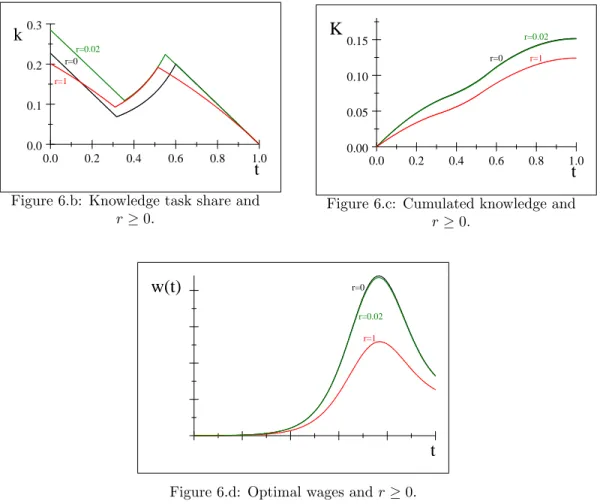
(31) K (t) =. 8 > < > :. rt. e. rD e. rtb. rT. e 1 + Ar t for t 2 [0; ta ) K0 + k0 Ar r rD e rt 1e rT for t 2 [ta ; tb ] A + r (t tb ) rA2 e r(T t) e r(T tb ) for t 2 (tb ; T ]. Solving for ta , tb ; k0 and D: We need four additional conditions to determine the values of ta , tb ; k0 and D. Since the state variable K is continuous at all t, hence at t = ta , this implies: erta 1 r. A r. K0 + k0. A ta = r. +. D : (ta ). (73). Assuming that k is continuous at t = ta , we have: A 1 r. k0 erta +. erta = r2 D. (e. e. rta. rta. e. (74). rT )2. Assuming that k is continuous at t = tb , we have: D. _ (tb ) ( (tb )). 2. =. A 1 r. e. r(T. tb ). :. (75). We need a fourth condition: using (60), (62) and (63), we …nd that, for all t 2 (ta ; tb ): _ (t) =. ' (t) =. Using (70) and (69), and using • = re _ (t). = =. rt. 1 _ A 1 _ A. Using _ (t) = 0 for all t 2 [0; ta ), we have. rk (t) .. r _ , we have. =. =. 1 _ (t) A + k_ (t) A (t). 1 _. _ A + 2D A. 2De. D 2 e A. re. 2. rt. e rT. _ 3. !. rT. e. rT. !. 2. _ rT 4. :. (76). (ta ) = (0) = 1. Using,. (tb ) = 0 and integrating (76) between. ta and tb , we …nd: (tb ). (ta ). = =. 1 0. Ztb. ta. B1 _ @. 2. D e A. 2. _ rT. Using integration by parts, this condition can be written as follows: " 1 (tb ) r3 D rT 3e rtb e rT 1 = ln e 3 (ta ) 3A (e rtb e rT ). 4. 1. C Ad . rta. 3e (e. rta. Solving for (73), (74), (75) and (77) provides the values of ta , tb ; k0 and D. 29. e e. rT rT )3. #. :. (77).