HAL Id: hal-02105528
https://hal.archives-ouvertes.fr/hal-02105528
Submitted on 21 Apr 2019
HAL is a multi-disciplinary open access
archive for the deposit and dissemination of
sci-entific research documents, whether they are
pub-lished or not. The documents may come from
teaching and research institutions in France or
abroad, or from public or private research centers.
L’archive ouverte pluridisciplinaire HAL, est
destinée au dépôt et à la diffusion de documents
scientifiques de niveau recherche, publiés ou non,
émanant des établissements d’enseignement et de
recherche français ou étrangers, des laboratoires
publics ou privés.
J. Oliveira, M. Wieczorek
To cite this version:
J. Oliveira, M. Wieczorek. Testing the axial dipole hypothesis for the Moon by modeling the direction
of crustal magnetization. Journal of Geophysical Research. Planets, Wiley-Blackwell, 2017, 122 (2),
pp.383-399. �10.1002/2016JE005199�. �hal-02105528�
Testing the axial dipole hypothesis for the Moon by modeling
the direction of crustal magnetization
J. S. Oliveira1 and M. A. Wieczorek1,2
1Institut de Physique du Globe de Paris, Sorbonne Paris Cité, Université Paris Diderot, CNRS, Paris, France,2Université Côte
d’Azur, Observatoire de la Côte d’Azur, CNRS, Laboratoire Lagrange, Nice, France
Abstract
Orbital magnetic field data show that portions of the Moon’s crust are strongly magnetized, and paleomagnetic data of lunar samples suggest that Earth strength magnetic fields could have existed during the first several hundred million years of lunar history. The origin of the fields that magnetized the crust are not understood and could be the result of either a long-lived core-generated dynamo or transient fields associated with large impact events. Core dynamo models usually predict that the field would be predominantly dipolar, with the dipole axis aligned with the rotation axis. We test this hypothesis by modeling the direction of crustal magnetization using a global magnetic field model of the Moon derived from Lunar Prospector and Kaguya magnetometer data. We make use of a model that assumes that the crust is unidirectionally magnetized. The intensity of magnetization can vary with the crust, and the best fitting direction of magnetization is obtained from a nonnegative least squares inversion. From the best fitting magnetization direction we obtain the corresponding north magnetic pole predicted by an internal dipolar field. Some of the obtained paleopoles are associated with the current geographic poles, while other well-constrained anomalies have paleopoles at equatorial latitudes, preferentially at 90∘ east and west longitudes. One plausible hypothesis for this distribution of paleopoles is that the Moon possessed a long-lived dipolar field but that the dipole was not aligned with the rotation axis as a result of large-scale heat flow heterogeneities at the core-mantle boundary.1. Introduction
We have learned from paleomagnetic studies of lunar samples collected during the Apollo missions that the lunar crust was magnetized in the presence of an ambient magnetic field with intensities at the surface greater than 10 μT [e.g., Fuller and Cisowski, 1987]. Though the time evolution of the field strength is not well constrained, current measurements suggest that these strong fields were present between about 4.2 and 3.6 Ga, with the possibility that weaker fields might have persisted much longer (see Weiss and Tikoo [2014] for a review). Magnetic field measurements obtained from orbit also show that there are strong magnetic anomalies of crustal origin distributed heterogeneously across the lunar surface. Though the initial orbital measurements obtained by Apollo only covered a small swath across the equator [Lin, 1979; Hood et al., 1981], more recent missions with polar orbits such as Lunar Prospector [Richmond and Hood, 2008; Mitchell et al., 2008; Purucker and Nicholas, 2010] and Kaguya [Takahashi et al., 2014; Tsunakawa et al., 2015] have extended these measurements globally.
Nonetheless, the origin of the field that magnetized the crust is still unresolved, and several competing ideas have been proposed. The hypothesis of a global field generated by a core dynamo is perhaps the most widely accepted [Hood, 2011; Shea et al., 2012; Weiss and Tikoo, 2014; Laneuville et al., 2014], but transient fields gen-erated (or amplified) during impact events have also been proposed [e.g., Hood and Artemieva, 2008; Hood
et al., 2013]. Even if the magnetic field was generated by the core, there are many aspects relating to such a
core dynamo that are still unknown. The power source for the dynamo is not known, with secular cooling, core crystallization [Laneuville et al., 2014; Scheinberg et al., 2015], precession [Dwyer et al., 2011], thermo-chemical mantle convection [Stegman et al., 2003], and impact-induced changes in the rotation rate [Le Bars
et al., 2011] all having being proposed. Furthermore, the geometry of such a field is not known. Though one
might presume that such a field would be predominantly dipolar, with the dipole axis approximately aligned with the rotation axis (such as for other rocky bodies, e.g., Earth, Mercury, and Ganymede), it has also been proposed that the dipole axis might draw circular paths as a result of lateral variations in heat flux at the
RESEARCH ARTICLE
10.1002/2016JE005199
Key Points:
• The direction of magnetization within the lunar crust was inverted using a unidirectional magnetization model • The paleomagnetic poles of several isolated anomalies are not randomly distributed, and some have equatorial latitudes
• The distribution of paleopoles may be explained by a dipolar magnetic field that was not aligned with the rotation axis Supporting Information: • Supporting Information S1 Correspondence to: J. S. Oliveira, oliveira@ipgp.fr Citation:
Oliveira, J. S., and M. A. Wieczorek (2017), Testing the axial dipole hypothesis for the Moon by modeling the direction of crustal magnetization, J. Geophys. Res. Planets, 122, 383–399, doi:10.1002/2016JE005199.
Received 13 OCT 2016 Accepted 4 FEB 2017
Accepted article online 9 FEB 2017 Published online 23 FEB 2017
©2017. American Geophysical Union. All Rights Reserved.
core-mantle boundary [Takahashi and Tsunakawa, 2009]. Finally, the duration of dynamo generation is not well constrained. Core crystallization, and perhaps precession, might be able to power a dynamo for several billion years, but dynamos driven by thermochemical mantle convection or generated by impact-induced changes in the rotation rate would only generate transient fields lasting from a few hundred million years to tens of thousands of years.
If the Moon possessed a core dynamo in its past, it is plausible that it would be largely dipolar with its sym-metry axis aligned with the lunar rotation axis. In this case, the direction of crustal magnetization would vary with planetary latitude, just as on Earth. This hypothesis can be tested by modeling the direction of crustal magnetization from spacecraft-derived magnetic field data. Once the direction of crustal magnetiza-tion is obtained, the corresponding locamagnetiza-tion of the north geomagnetic pole can be calculated, providing the so-called “paleopole” when the magnetic anomaly formed. If the paleopoles were all found to correspond to the present-day geographic poles, this would be consistent with a long-lived dipolar magnetic field gener-ated by a core dynamo. If the paleopoles clustered about two antipodal points, this could indicate that the field reversed polarity one or more times. If the paleopoles were found to all cluster about an axis that is offset from the current rotation axis, or if a quasilinear track of paleopoles were found, this could perhaps be con-sistent with a core-generated dipolar field but with a subsequent episode of true polar wander. Alternatively, if no coherent structure was found in the paleopole data, then this might indicate that either the core field was dominated by higher-order harmonics or that the field was derived from short-lived transient events associated with the impact cratering process.
Previous studies that have attempted to investigate the origin and direction of crustal magnetization have employed a variety of simplifying assumptions. These models have included the use of point dipoles [Takahashi et al., 2014], uniformly magnetized circular disks [Hood, 1981, 2011], and uniformly magnetized elliptical or circular prisms [Arkani-Hamed and Boutin, 2014] and were often applied to simple, isolated, clearly dipolar magnetic anomalies. In most cases, a single magnetic source was used to model the anomaly, though in a few cases [Hood et al., 1981; Hood, 2011; Takahashi et al., 2014] additional sources were used when more than one anomaly were in the region being investigated. In these types of models, strong assumptions need to be made about the source geometry and location. Though a best fitting solution can always be obtained, there are often significant residuals between the model and observations, and the appropriateness of the model assumptions is difficult to quantify.
In this work, we invert for the direction of crustal magnetization associated with isolated lunar magnetic anomalies using an approach originally developed by Parker [1991]. This method largely bypasses the non-uniqueness of previous studies associated with specifying the geometry of the magnetic sources. The only assumption is that the direction of crustal magnetization is constant within the crust, and no assumptions are made about the source geometry. The magnitude of crustal magnetization is allowed to vary both hori-zontally and over a range of depths. As a result of some simplifying theorems, Parker [1991] showed that this model is equivalent to one in which unidirectional equivalent source dipoles are placed at the surface and furthermore that the solution is easily obtained by a nonnegative least squares inversion. The assumption of unidirectional magnetization was used previously by Hemingway and Garrick-Bethell [2012] for two lunar anomalies and by Nayak et al. [2016] for anomalies in the northern edge of the lunar south pole-Aitken basin. In this work, we make use of a recent global magnetic field model based on Lunar Prospector and Kaguya data [Tsunakawa et al., 2015] and apply this technique to a larger number of lunar magnetic anomalies. We first describe in section 2 how the unidirectional magnetization model of Parker is applied to the Moon. Next, in section 3, using three anomalies with different behaviors as examples, we describe how we dis-cretize the problem, how we compute the model misfit, and how we estimate the uncertainty in the direction of magnetization. We then apply this approach to several anomalies and plot the resulting paleopoles. In section 4, we compare our results with previous studies and describe in more detail how the model assumptions of previous studies differ from ours. We then discuss several hypotheses that could account for our distribution of paleopoles, of which some are located at equatorial latitudes. Finally, we conclude by discussing how the origin and evolution of the lunar magnetic field could be addressed in future studies.
2. Method
In order to investigate whether the lunar crust was magnetized in the presence of an axial dipolar magnetic field, we investigate isolated magnetic anomalies located at several locations on the Moon’s surface. We use
the method described by Parker [1991] (called Parker’s method henceforth) that was previously used to study seamount magnetization on Earth. In contrast to previous studies, Parker’s method makes no assumptions about the geometry of magnetic sources but assumes only unidirectional magnetization inside the analysis region of volume V. In practice, the continuous distribution of magnetization is discretized using equivalent source dipoles, whose equivalent magnetic moment varies with position but whose direction is constant. The model magnetization can be written as
M(si) = ̂m m(si), m(si)≥ 0 , (1)
where ̂m is the unit direction of magnetization and m(si) is the dipole moment at vectorial position si.
In Parker’s original inversion of seamount magnetization on Earth, he chose to model only that component of the magnetic field that was aligned with the direction of Earth’s main geomagnetic field. Since the Moon does not have a main dipolar magnetic field at present, we will model only a single component in the direction ̂dj,
where the index j provides the latitude and longitude coordinates of the observation. As the component to be analyzed is arbitrary, we will use the radial component
̂dj=̂rj, (2)
but in our sensitivity tests, we will also consider the𝜙 and 𝜃 components.
The magnetic field d in direction ̂d at observation point j can be calculated as a sum of the contributions from the dipoles located at position si
dj= Nd ∑
i=1
gj(si) m(si), j = 1, … , No, (3)
where the contribution of a single dipole at location i is given by
gj(si) = 𝜇0 4𝜋 ( 3̂m ⋅(rj− si) ̂dj⋅ ( rj− si ) |rj− si|5 − ̂m ⋅ ̂dj |rj− si|3 ) . (4)
Noand Ndcorrespond to the number of observations and the number of dipoles in the crust, and rjand si are the vector positions of the observations and dipoles relative to a fixed planetocentric origin, respectively. As shown by Parker, the best fitting model in the least squares sense, subject to the constraint that m(si) is
positive, corresponds to no more than Nodipoles placed on the surface of the model domain. We emphasize
that no assumptions about the intensity of magnetized sources, source geometry, or statistical distribu-tions are made, which is the main strength of the method. Furthermore, the fact that the 3D distribution of magnetization is equivalent to a 2D distribution on the surface greatly simplifies the inversion approach. Equations (3) and (4) can be written in matrix form as
d = G(̂m) m , (5)
where the matrix G depends upon the assumed direction of magnetization ̂m, d is a vector of the observations projected in the direction ̂dj, and m is a vector that contains the (positive) magnitudes of the surface dipoles
at locations si. Following Parker [1991], we solve for m using the method of nonnegative least squares as
developed by Lawson and Hanson [1974]. As discussed in Parker [1991], one of the properties when using the nonnegative least squares technique is that if there are Nomagnetic field observations, then a maximum
of Noof the Ndsurface dipoles will be nonzero. In practice, we choose the number of surface dipoles, Nd, to be much larger than the number of observations, No. In this case, the nonnegative least squares technique automatically determines which surface dipoles have nonzero values.
For a specified direction ̂m, we determine the equivalent north geomagnetic pole, the locations of the surface dipoles that best fit those data, the surface dipole intensities, and the root-mean-square (RMS) misfit between the model and observations. To determine the best fitting direction, we vary ̂m over all directions on the unit sphere. With a plot of the misfit as a function of the magnetization direction, the best fitting direction is obtained. Furthermore, given the value of a maximum acceptable misfit, the uncertainty in the magnetization direction is obtained simply by plotting the contour of the maximum allowable misfit.
We choose to model isolated sources, where the field surrounding the magnetic anomaly is weaker than the anomaly itself. Our approach for defining the maximum allowable misfit is based on the concept that the residual unmodeled magnetic field should be statistically similar to the “background” field surrounding the anomaly. The background in this case could either be measurement noise or that portion of the signal that is inconsistent with the assumption of unidirectional magnetization. In practice, we define the 1 sigma error ellipse of the magnetization direction as those directions whose RMS misfit is less than or equal to the RMS background field. In all cases, the strength of the residual field is found to be considerably smaller than the field strength of the anomaly being modeled.
This approach for defining the misfit has two potential problems. First, if the background magnetic field had a high amplitude with respect to the central magnetic anomaly, the range of allowable magnetization directions would be large. If the background field was uniform in direction, it might be possible to first sub-tract the background field before doing the analysis. Nevertheless, the wisdom of modeling a weak anomaly surrounded by stronger sources would need to be carefully assessed. To avoid such complications, we only consider isolated anomalies that are surrounded by weaker fields. Second, if the surrounding fields were extremely weak, then the uncertainties would conversely be very small. In this case, if the central mag-netic anomaly had large amplitudes, and if small signals existed that were inconsistent with unidirectional magnetization, it might not be possible to fit the observations to the level of the background field.
3. Analysis of Isolated Magnetic Anomalies
We use the gridded magnetic field models of Tsunakawa et al. [2015] that are based on vector magnetic field measurements made by the Lunar Prospector and Kaguya missions (see Figure 1). In their model, the radial magnetic field was inverted on a regular grid on the surface with a spatial resolution of 0.2∘. From this gridded data set, the three components and total intensity were calculated on a regular grid with a 0.5∘ resolution at 30 km altitude through forward modeling procedures (see Tsunakawa et al. [2014] for details). In this study, we will make use primarily of the radial component maps at 30 km altitude, but we will also perform sensitivity tests using the other components and the surface data. Given that the two horizontal components of the magnetic field were derived exclusively from the radial component, the use of a single component in our inversion makes use of all information in their data set.
We examine most of the isolated anomalies that have been investigated in previous works [e.g., Arkani-Hamed
and Boutin, 2014; Takahashi et al., 2014]. Figure 1 labels those anomalies that are discussed in the text. Though
some of these anomalies have simple dipole-like signatures, others are clearly composed of extended sources. These anomalies are well distributed across over the Moon’s surface possessing a range of geographic lati-tudes and longilati-tudes. A few anomalies that were studied by Arkani-Hamed and Boutin [2014] and Takahashi
et al. [2014] are not reported here, as they were not sufficiently isolated to be treated in our analysis.
In this section, we first describe all relevant steps involved in our inversion and uncertainty analyses. Following this, we describe in detail the results for three anomalies with contrasting behaviors: Reiner-𝛾, Descartes, and Airy. After highlighting the potential problems with such inversions, we then present our results for all investigated anomalies and describe the characteristics of the obtained paleopoles.
3.1. Model Description
For a given magnetic anomaly, we start by placing dipoles on the surface using a homogeneous polar coordi-nate distribution [Katanforoush and Shahshahani, 2003] with a 0.4∘ resolution. The dipoles are placed within a circle of angular radius rdthat is centered on the anomaly and whose size depends on the extent of the
anomaly being investigated. Note that the chosen grid spacing at the surface (0.4∘) is smaller than the grid spacing of the data (0.5∘) at 30 km altitude.
The modeled magnetic field data were compared to the observations within a second circle of radius ro.
The radius of this circle was chosen to be somewhat larger than that of rdwhere the dipoles were placed in
order to avoid unwanted edge effects. In particular, given the well-known nonuniquenesses associated with potential-field modeling, a central isolated magnetic anomaly could correspond to either a region of strong magnetization in an unmagnetized crust or a region of no magnetization in a uniformly magnetized crust. As shown later, if the misfit between observations and model where calculated using ro= rd, strong
mag-netic anomalies related to edge effects could occur just outside of the region where the misfit was calculated. In this study, we make the assumption that the crust is on average not magnetized, with the exception of the
Figure 1. Magnetic field strength of the Moon at 30 km altitude
from the 0.5∘gridded data of Tsunakawa et al. [2015] based on Lunar Prospector and Kaguya observations. White circles indicate the locations of the magnetic anomalies investigated in this study. Data are presented in a global Molleweide projection, centered on
the 0∘meridian.
isolated anomaly within the analy-sis region. To penalize the existence of such edge effects associated with distributions of surface dipoles that approximate a uniformly magnetized crust, we calculate the misfit within a circle rothat is larger than rd. For our
nominal models, we use ro= rd+ 1∘
of angular distance along a great cir-cle (except for one case where 1.5∘ is used instead of 1∘), noting that 1∘ (∼30 km) corresponds approximately to the distance between the surface and measurement altitude. A sensitiv-ity test that uses different values will be addressed in the following section. For a given direction of magnetiza-tion, we next perform a nonnegative least squares inversion [Lawson and
Hanson, 1974] in order to determine the locations of the dipoles with nonzero magnetic moments, their
intensities, the predicted magnetic field, and the RMS misfit between the data and observations. We vary the magnetization direction over all directions using a planetocentric unit vector that is varied over a 2∘ equidis-tant grid in latitude and longitude. For each magnetization direction, the corresponding north paleopole is calculated using equations modified from Butler [1992] (note that for historical reasons, it is common in the terrestrial literature to cite the south magnetic pole). Finally, we plot the model misfit as a function of both magnetization direction and north paleopole location. We note that since we use more dipole locations on the surface than observations, many of the dipole locations are associated with a zero magnetic moment. By having more dipole locations than observations, this provides more liberty for the nonnegative least squares routine in choosing the locations that best fit the data.
We determine the uncertainty of our paleopole locations by making use of a maximum allowable RMS misfit between model and data. One possible measure of the misfit is the uncertainty in the magnetic field mea-surement itself. For the Lunar Prospector and Kaguya data, this corresponds to about 0.05 nT, which is much smaller than other sources of error. Another possibility is to use the uncertainty in the radial magnetic field as obtained in the inversions of Tsunakawa et al. [2015]. For this case, only a single uncertainty was provided for each analysis region (with a representative size of 15∘ in latitude and longitude). These formal uncertain-ties are on the order of 1.5 nT on the surface and are found in practice to be much larger than our model uncertainties. We suspect that the largest source of uncertainty in our model is not the uncertainty in the data themselves, or from unmodeled solar wind fields and lunar interactions, but rather small geologic signals that are inconsistent with our model assumptions. For example, if some portion of crustal magnetization were not unidirectional, it would be unlikely that the unidirectional magnetization model [Parker, 1991] would be able to fit the observed field.
As described in section 2, we thus take the approach that after our model is subtracted from the data, the RMS misfit should be comparable to the amplitude of the magnetic field that surrounds the isolated anomaly. This is a very conservative approximation, as it assumes that the ambient field is “noise” that is uncorrelated with the region being modeled. As a representative measure of this background field, we take the RMS of the measurements that are found between the two circles of radii roand rd.
3.2. Reiner-𝜸, Descartes, and Airy
We demonstrate our approach by inverting for the magnetization direction of three prominent magnetic anomalies on the nearside of the Moon: Reiner-𝛾, Descartes, and Airy. As is the case for most magnetic anoma-lies, these have no clear, unambiguous association with any known geologic feature or process. In Figure 2, the first column plots the observed radial magnetic field along with the points used in calculating the misfit; the second column plots the best fit model, along with the locations of the surface dipoles; the third column plots the difference between the two; and the fourth column plots the intensity of the magnetic moments of
Figure 2. (first column) Observed radial magnetic field, (second column) the best fit model magnetic field, (third column)
the difference between observations and modeled magnetic field, and (fourth column) the magnetic moments of the retained dipoles in the inversion for the (a) Reiner-𝛾, (b) Descartes, and (c) Airy magnetic anomalies. For each anomaly, the data points (within the outer circle) and the locations of dipoles (within the inner dashed circle) used in the inversion are denoted by dots in Figure 2 (first and second columns). The misfit between observations and model is computed using the data points within the outer circle.
the best fitting surface dipoles. The two circles of radii roand rdthat delimit the locations of the observations
and surface dipoles are plotted in each image, and the fourth column also plots a topographic shaded-relief map of the region for geologic context.
As is evident from Figure 2, our model of unidirectional magnetization fits well the observations. The best fitting RMS misfit values are 0.61 nT, 0.58 nT, and 0.31 nT for the Reiner-𝛾, Descartes, and Airy anomalies, respectively, which compare favorably with the RMS values of the ambient magnetic field of 0.56 nT, 0.79 nT, and 0.71 nT between the two circles of radius roand rd. The nonnegative least squares solution provides the
magnetic moments and position of the dipoles, and in general, these are seen to be highly correlated with the regions that have the strongest magnetic fields. Though the anomalies have dipolar appearances, the model is capable of accurately accounting for more complex structures, such as the anomaly found northeast of Reiner-𝛾. In these three examples, no apparent correlation is found between the intensity of the surface dipole moments and topography.
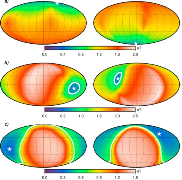
In Figure 3, we plot the misfit as a function of the magnetization direction (parameterized as a unit vector placed at the center of the planet), as well as the corresponding location of the north magnetic pole. As an
Figure 3. Misfit as a function of (left column) magnetization direction in planetocentric coordinates and (right column)
north paleomagnetic pole position with the corresponding uncertainty denoted by a white solid line for (a) Reiner-𝛾, (b) Descartes, and (c) Airy magnetic anomalies. The star denotes the best fitting solution. Results are presented using a global Molleweide projection with a central meridian of 0∘.
example, for Reiner-𝛾, which is located near the equator, the magnetization direction is tangential to the surface and points toward the north. For this case, it is easy to infer geometrically that the north geomag-netic paleopole is located near the south geographic pole. This result is consistent with the hypothesis that the Moon once possessed a global core dynamo generated field that was predominantly dipolar and aligned with the Moon’s rotation axis. For this case, the best fitting RMS misfit of 0.61 nT corresponds almost exactly to the ambient value of 0.56 nT, precluding us from plotting an error ellipse.
Contrary to this result, the north magnetic poles of the Descartes and Airy anomalies are located at 20∘N and 42∘N latitude, respectively, which are far from the present geographic poles and therefore not consistent with a dipolar magnetic field aligned with the rotation axis. For Descartes, the uncertainty in the paleopole is fairly small, corresponding to a circle with an angular radius of about 15∘ of latitude. In contrast, for the Airy anomaly, directions of magnetization that cover almost half a hemisphere can fit the data using our definition of the uncertainty. For this anomaly, even though the assumption of unidirectional magnetization is justified, and even though we can place bounds on the distribution and intensity of magnetization in the crust, little definitive information about the magnetization direction can be obtained. Part of the reason for this is that the intensity of this magnetic anomaly is somewhat less than that of the other two. Nevertheless, we emphasize that our estimate of the uncertainty is conservative and that we might potentially overestimate the allowable range of magnetization directions.
Figure 4. Best fitting radial magnetic field models for the Reiner-𝛾anomaly using differences between the radiirdand
roof (from left to right) 0∘, 0.5∘, 1∘, and 1.5∘. Dots within the inner dashed circle of angular radiusrd=6∘denote the surface dipole positions. The solid outer circle delimits the region used to calculate the misfit.
3.3. Sensitivity Analysis
Before presenting the paleopole results for the other magnetic anomalies in our study, we discuss how var-ious assumptions of our modeling approach might affect the final results. First, we tested how the results depended upon the relative sizes of the two circles roand rd. As a demonstration of undesirable edge effects,
in Figure 4 we plot the best fitting magnetic field models for Reiner-𝛾, where the difference in radius of the two circles was 0, 0.5, 1, and 1.5∘ (see supporting information for details). As is seen, for the cases of 0 and 0.5∘, even though the data are well fitted in the analysis region, large signals are predicted just exterior to the region being fitted. These edge effects are not seen when the difference in circle radii is 1 and 1.5∘. Inversions that made use of a 1.5∘ separation were found to provide nearly identical paleopole locations, with only slightly different uncertainties.
Second, we have tested whether use of the𝜃 and 𝜙 components of the magnetic field, each individually, provide similar results as obtained from the radial component. Inversions using these two components for the Reiner-𝛾 and Descartes anomalies provide results that were found to be largely comparable, both in terms of best fit paleopoles and uncertainties (see supporting information). Though the results are not always exact, differences in paleopole locations were on the order of only 1 to 4∘. Using the horizontal components in the
Table 1. Location (Lon, Lat), Radii of Observations (ro) and Dipoles (rd), Number of Observations (No) and Dipoles (Nd) Used in the Inversion, the Number of Nonzero Dipoles (Nzd) of the Best Fitting Calculated Model, Magnetization Direction in Planetocentric Coordinates (𝜙m, 𝜃m), North Paleopole Position (𝜙p, 𝜃p), the RMS Misfit Between the Best Fitting Model and the Data, and the Corresponding RMS Signal Between the Radiiroandrd(𝜎)a
Anomaly Lon (deg) Lat (deg) ro(deg) rd(deg) No Nd Nzd 𝜙m(deg) 𝜃m(deg) 𝜙p(deg) 𝜃p(deg) Misfit (nT) 𝜎(nT) Abela 87.5 −31.0 8 7 932 1192 375 14.0 −75.7 107.6 37.9 0.39 0.67 Airy 3.1 −18.2 5 4 316 375 103 216.6 −10.9 113.9 42.2 0.31 0.71 Crisium 58.5 17.3 9 8 1012 1490 519 254.4 −64.0 225.9 47.5 0.37 0.96 Crozier 51.4 −15.4 5 4 314 377 137 223.8 3.6 249.1 36.7 0.27 0.56 Descartesa 16.0 −10.7 6.5 5.5 524 725 167 129.8 −13.7 278.9 20.3 0.58 0.79 Hartwiga 280.0 −9.0 9 8 1009 1542 480 239.4 21.1 348.1 −38.0 0.26 0.37 Kolhorster 247.0 13.0 8 7 797 1167 196 89.9 41.0 352.1 −69.9 0.38 0.57 Mendel-Rydberg 264.0 −51.0 8 7 1281 1195 418 187.8 −54.4 310.3 −1.9 0.22 0.47 Necho 124.0 −7.0 4.5 3.5 257 302 97 324.9 32.4 271.5 −34.1 0.33 0.83 Reiner-𝛾a 302.7 7.6 8 7 805 1190 182 149.3 77.1 348.7 −82.0 0.61 0.56 Scheiner 335.0 −62.0 5 4 667 390 140 299.8 −20.5 93.6 −41.1 0.14 0.42 Serenitatis 18.5 33.0 4.5 3.0 300 217 87 207.6 −10.5 157.4 −67.2 0.22 0.33 Sirsalis 303.0 −10.0 6 5 441 601 165 109.3 −14.5 155.2 48.2 0.38 0.87 Smythii 87.5 0.0 4.5 3.5 249 300 84 53.1 −32.6 141.4 42.5 0.304 0.54 Sylvestera 288.0 80.0 5 4 1848 385 92 102.2 5.9 282.2 −12.0 0.365 0.61
Figure 5. Misfit as a function of north paleomagnetic pole position with the corresponding uncertainty denoted by a
white solid line, (left column) for Sylvester, Abel, and Hartwig and (right column) for Sirsalis, Mendel, and Serenitatis. Results are presented in a global Molleweide projection with a central meridian of 0∘.
inversions for the Airy anomaly obtains a different best fit paleopole position that differs by about 80∘ from that of the radial inversions, but that is consistent within the uncertainties of the inversion. For all anomalies, the uncertainty ellipses using the horizontal components are largely consistent with those obtained from the radial component.
Third, we have performed inversions using different spacings for the dipoles on the surface. Our nominal model used a spacing of 0.4∘, and we tested spacings of 0.2 and 0.8∘. The results were nearly identical, but as expected, the smaller grid spacing of 0.2∘ provided somewhat lower RMS misfits than those from grids with the larger spacings (see supporting information).
Lastly, in addition to using the magnetic field model of Tsunakawa et al. [2015] at 30 km altitude, we have also performed inversions using their surface magnetic field model. Given that the surface data are provided using a much higher spatial resolution (0.2∘ as opposed to 0.5∘ for the 30 km altitude data), the matrix G in equation 5 was considerably larger and took more resources to invert. We found nearly identical results, with the paleopole location differing by only about 10∘ from that obtained from the 30 km altitude data
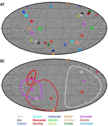
Figure 6. North (filled symbols) and south (empty symbols)
paleomagnetic pole positions for (a) all studied crustal magnetic anomalies and (b) the best constrained anomalies with corresponding 1𝜎uncertainties. The two maps are in a Molleweide projection centered at 0∘E, and the analyses and anomaly names are coded by color.
(see supporting information for details). This is not surprising given that the 30 km altitude model is derived directly from the surface model.
3.4. Distribution of Paleopoles
In Table 1, we provide all data for the ano-malies that were investigated in this study. This includes the central location, the radii of roand rd, the number of observations,
the number of dipoles, the number of non-zero dipoles from the inversion, the RMS misfit, and RMS signal between roand rd.
Of the 15 anomalies investigated, only five paleopoles have uncertainties that are small enough to constrain models of the lunar magnetic field. These are Reiner-𝛾, Descartes, Sylvester, Hartwig, and Abel. The best fitting paleopoles and paleopole misfit for the Reiner-𝛾 and Descartes anomalies were previously shown in Figure 3. We provide the paleopole mis-fit plots for the remaining anomalies in Figure 5. As is seen, in addition to Descartes, the Sylvester anomaly also has a well-constrained paleopole that is also located close to 90∘W longitude and near the equator. Hartwig and Abel pro-vide weaker constraints on the paleopole location, but they too are not aligned with the geographic poles.
The best fitting north paleomagnetic poles for all anomalies investigated are plotted in Figure 6. We addition-ally plot the corresponding south magnetic paleopoles in order to take into account the possibility of reversals where the polarity of the dynamo generated magnetic field changes. This hypothesis has been used by other studies when investigating both Martian and lunar crustal magnetic anomalies [e.g., Takahashi et al., 2014;
Arkani-Hamed, 2001]. Though many of these paleopoles have large uncertainties, our approach for estimating
the uncertainty is conservative. We suspect that the real uncertainties are likely to be considerably smaller and that the distribution of best fitting directions, in addition to those with well-constrained uncertainties, provides guidance for interpreting the origin of the lunar magnetic field. In Figure 6b, for comparison, we plot only those paleopoles that are well constrained, their uncertainties, and corresponding south magnetic paleopoles.
As seen in Figure 6 the paleopoles are not clustered at the geographic poles and appear to not be distributed randomly over the lunar surface. Though a few paleopoles are found to be close to the current geographic poles, such as Reiner-𝛾, Kolhorster, and Serenitatis, the vast majority are not. These three paleopoles are all associated with the south geographic pole and hence do not require magnetic reversals to have occurred. There are almost no paleopoles within the central nearside, corresponding to the region that has been resur-faced by mare basalt lava flows. Similarly, very few paleopoles are associated with the central farside highlands. Many of the paleopole positions are found to be located close to 90∘E and 90∘W longitude.
Of the best fitting paleopoles, one is clearly located at the south geographical pole (Reiner-𝛾), another is barely consistent with being located at the south geographical pole (Hartwig), and three are consistent with having equatorial latitudes with longitudes close to 90∘W and 90∘E. Thus, our data seem to be inconsistent with the hypothesis that the Moon possessed a dipolar magnetic field aligned with the rotation axis. The pale-opole locations, however, do not appear to be random, suggesting that the field was in fact organized in some manner. This nonrandomness in paleopole locations suggests that transient magnetic fields associated
with impact events are not responsible for most crustal magnetization. There is a notable lack of pale-opoles within the lunar maria, which also correspond to the Procellarum KREEP Terrane [Jolliff et al., 2000;
Wieczorek and Phillips, 2000], a region that contains high abundances of heat-producing elements. The
non-uniform distribution of paleopoles suggests that while the main field might have been dipolar, the dipole axis was not predominantly aligned with the rotation axis. The dipole axis could perhaps have circulated in a great circle path along 90∘W and 90∘E longitudes or perhaps might simply have avoided the region associated with the lunar mare and Procellarum KREEP Terrane.
4. Discussion
4.1. Comparison With Previous Studies
In this work, we have made use of the unidirectional magnetization model of Parker [1991] to study isolated lunar magnetic anomalies. As discussed in section 2, this model makes no assumptions about the geometry of the magnetic sources and assumes only that the direction of magnetization within the crust is constant in direction. Given that there are many degrees of freedom in our inversion (including the location and inten-sity of a large number of magnetic sources at the surface), we can always find models that adequately fit the observations. Unfortunately, because of the large number of degrees of freedom, the magnetization direction is not well constrained for many anomalies. For the most poorly behaved anomalies (such as Airy), the magnetization direction can either be entirely unconstrained or constrained to lie within one hemisphere. Nevertheless, given the weak assumptions in Parker’s method, when the magnetization direction is well constrained, this can be taken as a robust result.
Several studies have been published over the past four decades that have investigated the direction of lunar crustal magnetism. For the most part, these make use of simplifying assumptions about the source geometry and source location. A single or small number of point dipoles are often employed, and in some cases mag-netized disks have been used. Given the small number of degrees of freedom, these models usually obtain a well-defined best fitting magnetization direction with small error bars (when uncertainties are reported). However, the robustness of the inverted magnetization direction depends strongly upon the assumptions made by the model, and these assumptions are rarely, and not easily, quantified. Though the results pre-sented in those studies might be correct, they could be in error if the actual source geometry differed from the assumption.
A few studies that investigated the direction of lunar crustal magnetization were published using orbital mag-netic field data obtained from the Apollo 15 and 16 missions [Hood et al., 1981]. These data spanned two great circle swaths that were slightly inclined with respect to the equator, limiting the number of anoma-lies that could be investigated. Here we note simply that the crustal anomaanoma-lies were, in general, modeled by isolated dipoles and that the corresponding paleopoles spanned a large range of directions. By group-ing the paleopoles by surface age (which does not always correspond to the age when magnetization was acquired, especially when the magnetization is deep within the crust), it was argued by Runcorn [1983] that the paleopoles were somewhat clustered and that significant true polar wander might have occurred. Following the acquisition of data from the Lunar Prospector mission, a number of these analyses were reassessed. Richmond et al. [2003] modeled the nearside Descartes anomaly by a circular disk. From their reported inclination and declination (no uncertainties were reported), we obtain a paleopole location of 8∘S and 273∘E. Situated 28∘ away from our best fitting paleopole, their paleopole position lies outside of our uncertainties of about 7∘. Hood [2011] investigated the direction of magnetization associated with two promi-nent anomalies within the interior of the Crisium impact basin. For the northern anomaly, he obtained a paleopole close to the north pole (81∘N, 143∘E), but the southern anomaly had a much different paleopole that was located at low latitudes (38∘N, 90∘E). In our analysis, we did not investigate each of these two anoma-lies separately but rather performed an inversion over the entire basin. As shown in Le Bars et al. [2011], the impact melt sheet and remaining crust within the interior of the Crisium basin would have cooled below the Curie temperature in a few tens of thousands of years, and it is reasonable to expect that the direction of the magnetizing field would have been constant over this time interval. Our model can fit both Crisium anomalies using a single direction of magnetization, but the obtained paleopole is, not surprisingly, much different than those obtained for the northern and southern anomalies in the analysis of Hood [2011].
Hemingway and Garrick-Bethell [2012] used an approach similar to Parker [1991] to investigate the Airy and
In contrast to our study that made use of a nonnegative least squares inversion to solve the problem, they employed a genetic algorithm to explore the parameter space. They did not investigate whether their best fitting model predicts edge effects exterior to the region being modeled. Nevertheless, from their best fitting inclination and declination for Reiner-𝛾 (no uncertainties provided), we obtain a paleopole of (79∘S, 353∘E), which differs from ours by only 3∘. In contrast, their inclination and declination for the Airy anomaly imply a paleopole of (8.4∘S, 353∘E), which is much different than our best fitting value. Regardless, the difference of 74∘ between their and our best fitting results is consistent within our uncertainties for this anomaly. Given that the direction of magnetization for the Airy anomaly is only poorly constrained in our inversion, this comparison highlights the importance of calculating robust uncertainties for the direction of magnetization.
More recently, there have been two studies that have made use of data collected by both Lunar Prospector and Kaguya. In Takahashi et al. [2014], 15 magnetic anomalies were modeled using (for the most part) a sin-gle dipole source representation for each anomaly. The location, inclination, declination, and dipole moment were solved for, and formal uncertainties were obtained using the RMS residual of the best fitting model as an estimate of the noise in the magnetic field. With an uncertainty for the inclination and declination, an error ellipse was obtained for the paleopole. For a few cases where more than one anomaly was located in the analysis region, additional dipoles were added to the inversion. Only 14 anomalies were retained for inter-pretation, and just under half of their paleopoles clustered at the north and south geographic poles. The remainder spanned a wide range of latitudes and about 90∘ of longitude (when all poles are projected in one hemisphere). From these results, the authors suggested that the Moon had a reversing dipolar magnetic field and that 45–60∘ of polar wander occurred while the dynamo was operating.
Of the 14 anomalies investigated by Takahashi et al. [2014], only 10 can be compared with ours. The anomalies Reiner-𝛾, Descartes, and Serenitatis have comparable paleopoles with an angular difference of 7∘, 10∘, and 25∘, respectively. Though their results for Descartes are consistent with ours, they excluded this anomaly in their interpretations as it represented an outlier in their paleopole locations and also because this anomaly might be related to impact ejecta that was magnetized by transient impact-generated fields [see also Richmond et al., 2003]. Though the surface materials in the Descartes region probably do represent ejecta from the Nectaris impact basin, we note that the majority of Nectaris ejecta is not magnetized and that it is equally plausible that this magnetic anomaly formed before the Nectaris impact. Their best fitting paleopoles for Smythii, Crozier, Kolhorster, Necho, Sirsalis, and Serenitatis differ from ours but are consistent within the large uncertainties of our analysis. Only for one anomaly, Airy, do we obtain a paleopole and corresponding uncertainty that disagrees with their results.
Finally, we note that Arkani-Hamed and Boutin [2014] also inverted for magnetization directions for 10 isolated magnetic anomalies. Elliptical prisms were used to model the anomalies. Though this study does not report uncertainties for the paleopole locations, several inversions were performed for each anomaly using different subsets of data and assumptions, providing information about the sensitivity of the model parameters in the inversion. Similar to our results, their paleopoles span a large range of latitudes and longitudes but are not ran-domly distributed. Of the anomalies studied, six are in our study. The anomalies Reiner-𝛾, Scheiner, Sylvester, and Hartwig have best fit paleopoles that compare well with ours, with angular differences of about 4, 8, 3, and 25∘, respectively. In particular, the best fit paleopoles for the Mendel, Hartwig, Scheiner, and Sylvester anomalies are consistent within the large uncertainties of our analysis. However, their paleopole for the Abel anomaly disagrees with our results and uncertainties.
4.2. Distribution of Paleopoles
Our distribution of paleopoles is not entirely consistent with the hypothesis that the Moon once possessed a dipolar magnetic field aligned with the rotation axis. Even though our best constrained inversions show that some paleopoles are located close to the present-day geographic poles, others are not. Previous studies that investigated the direction of crustal magnetism have noted the same behavior [e.g., Runcorn, 1980, 1982;
Takahashi et al., 2014; Arkani-Hamed and Boutin, 2014], but as discussed above, it is sometimes difficult to
compare the various studies, and the clustering of paleopoles is not always comparable between studies. Regardless, these studies agree that a significant fraction of magnetic anomalies have associated paleopoles that are far from the rotation axis, and this requires an explanation. In this section, we discuss several pos-sibilities that could account for the observed distribution of paleopoles, including the possibility that the anomalies are related to transient impact-generated fields, that the main field was not dipolar, that true polar wander has occurred, and that the dipole axis was not always aligned with the rotation axis.
4.2.1. Impact-Generated Fields
One possibility for the distribution of paleopoles is that the magnetizing field was not due to a core-generated field but rather transient magnetic fields associated with impact cratering events. For example, it has been suggested that an expanding plasma cloud during a basin-forming impact could amplify ambient magnetic fields preferentially at the antipode of the basin [Hood and Huang, 1991; Hood and Artemieva, 2008]. It has been suggested that impact events themselves might generate short-lived transient magnetic fields that could per-haps magnetize crater ejecta [Crawford and Schultz, 1988, 1989]. Finally, it has been suggested that cometary impacts, or the interactions of cometary coma with the lunar surface, could generate transient magnetic fields that might magnetize the crust [Schultz and Srnka, 1980].
The above mechanisms for field generation and amplification contain many aspects that are not well under-stood and modeled. Nevertheless, as a result of the stochastic nature of impact events, ambient solar wind fields, and the random distribution of craters on the surface of the Moon, it is unlikely that these events would give rise to any preferential distribution of magnetization directions within the crust. With no preference for magnetization direction, the paleopole locations would be random given the random locations of impact craters on the Moon. This expectation, however, is not consistent with our results, which show a preference for paleopoles along 90∘W and 90∘E longitudes and a deficit of paleopoles in the vicinity of the nearside maria and the Procellarum KREEP Terrane.
None of our anomalies are associated with a known antipode of an impact basin. Even if some of the anomalies in our study might be associated with a basin impact melt sheet (Crisium) or basin ejecta (Descartes), these thick deposits would require significant time to cool through the Curie temperature of metallic iron, during which time the transient fields would have dispersed [e.g., Le Bars et al., 2011]. Though we cannot dismiss the possibility that impact-related processes might have caused some large-scale magnetic anomalies, based on our analysis it is unlikely that this process is responsible for the majority of lunar magnetic anomalies.
4.2.2. A Multipolar Magnetic Field
In the process of calculating a paleopole from the direction of crustal magnetization, the underlying assump-tion is that the magnetizing field was predominantly dipolar. This is a reasonable assumpassump-tion given the strongly dipolar nature of the magnetic fields of Mercury, Earth, and Ganymede, all of which are generated by dynamo processes in their metallic cores. Nevertheless, numerical simulations show that dynamo-generated fields can be dominated by higher-order multipole terms under certain ranges of parameters [e.g., Olson and
Christensen, 2006; Christensen and Aubert, 2006], and it is not evident if a lunar dynamo would always have
been dominated by the dipole term. Even if the field was predominantly dipolar, depending on their strength, the presence of higher-order terms could still bias the calculated paleopoles.
If a dynamo was dominated by a single multipolar component, this could magnetize the crust in a coherent way that might give rise to a nonrandom distribution of paleopoles. As an example, we assumed that the magnetizing field corresponded to the sine, degree 2 order 1 Gauss coefficient (h1
2) and calculate the global magnetic field on a regular grid. As shown in Figure 7, the distribution of paleopoles (calculated under the assumption of a dipolar field) follow closely a great circle about 90∘W and 90∘E longitude. This scenario would be consistent with the paleopoles obtained in this study. However, lacking an asymmetric forcing term, even if the dynamo field was dominated by the quadrupole terms, on average, one would expect the energy to be partitioned evenly among all five degree 2 Gauss coefficients. If this were the case, paleopoles calculated under the assumption of a dipolar field would not give rise to any preferential distribution.
Even if the field was dominated by the dipole term, planetary dynamos are known to change polarity. For Earth, the dynamo spends most of its time in a single polarity and reverses in a period of time that is short in comparison to that of a given polarity. However, based on numerical simulations, by varying the driving parameters, the frequency of reversals could be much more frequent than for that of Earth [Driscoll and Olson, 2009]. The possibility exists that the lunar dynamo might have reversed more frequently than for Earth, and that some crustal anomalies might have acquired a remanent magnetization when the dipole term was not dominant. Nevertheless, as long as there was no single higher-order Gauss coefficient that was preferred dur-ing reversals of the lunar field, we would expect the paleopoles associated with rocks that cooled durdur-ing such events to be random in direction.
4.2.3. True Polar Wander
One possible explanation for the range of paleopole latitudes in our study, as well as the apparent clustering along 90∘W and 90∘E longitudes, is that the Moon underwent significant amounts of true polar wander when
Figure 7. Distribution of paleopoles calculated under the assumption of a
dipolar field, for a Gauss coefficienth12magnetic field. The map is in a Molleweide projection centered at 0∘E.
a lunar dynamo was operating. True polar wander has been invoked sev-eral times in the literature, but most studies only predict modest reori-entations. For example, Keane and
Matsuyama [2014] have shown that
the redistributions of mass associated with large impact basins, particularly the ancient south pole-Aitken impact basin, could have driven about 15∘ of true polar wander. This amount, how-ever, is insignificant to what is required to explain our paleopoles. A larger true polar wander of 36∘ was found by
Garrick-Bethell et al. [2014] using estimates of the degree 2 shape and gravity of the Moon after excluding
impact basins. More recently, using an apparent path of higher than average hydrogen abundances near the poles of the Moon, Siegler et al. [2016] have argued for a more modest true polar wander of about 6∘, oppo-site in direction of that of Garrick-Bethell et al. [2014] and approximately orthogonal to what was proposed by
Keane and Matsuyama [2014].
To account for the equatorial paleopoles in our study, approximately 90∘ of true polar wander would be required. This could be accomplished by the phenomenon of inertial interchange true polar wander [e.g., Piper, 2006], when the equatorial moment of inertia B (aligned in direction of the lunar orbit) becomes larger than the axial moment of inertia C. Though such large amounts of polar wander could potentially be accounted for by models that take into account the cooling of the Procellarum KREEP Terrane over time [Siegler et al., 2016], that model predicts the pole to follow a great circle path along 30∘ W longitude, which differs by about 60∘ from what is required by our observations. Current models of true polar wander are thus not consistent with our observations.
4.2.4. A Dipolar, Nonaxial Magnetic Field
Another possibility for the distribution of paleopoles obtained from our analysis is that the Moon once had a dipolar magnetic field generated by a core dynamo but that the symmetry axis of the dipolar field was not always aligned with the rotation axis. In one model, Aubert and Wicht [2004] have shown numerically that equatorial dipolar fields can indeed arise under a certain range of parameters but that these dynamos have weaker field strengths than their axial counterparts. In another model, Takahashi and Tsunakawa [2009] imposed a difference in heat flux at the core-mantle boundary between the nearside and farside hemispheres. The assumptions of this model were justified by the fact that the Moon’s thermal evolution differed between the near and farside hemispheres and that the majority of the Moon’s heat-producing elements are found on the nearside hemisphere in the Procellarum KREEP Terrane [e.g., Hess and Parmentier, 1995; Zhong et al., 2000;
Wieczorek and Phillips, 2000; Zhang et al., 2013; Laneuville et al., 2013, 2014]. Their models show that in such
a situation, the magnetic field would have been predominantly dipolar but that the axis of the dipole would have circulated in a great circle path.
Even though the model of Takahashi and Tsunakawa [2009] is consistent with our paleopole results, one poten-tial problem concerns the timescale of their circulating dipolar field. For the simulation in their paper, the timescale was about 60–70 years, which is much shorter than the cooling timescales of thick sequences of magmatic rocks. If the major magnetic anomalies are the result of kilometer-scale impact melt and ejecta deposits, or magmatic intrusions deep in the crust, it is unlikely that the crust would have been unidirection-ally magnetized, as is required by the model of Parker [1991]. Since only a single simulation was presented in their work, it is possible that a more systematic exploration of the parameter space in their model might allow for longer timescales of the circulating dipolar field.
Finally, we note that most numerical dynamo models are driven by secular cooling of a fluid core or by com-positional convection associated with core crystallization. It is possible that other more exotic power sources might power a lunar dynamo and that they might prefer different magnetic field geometries. In particular,
precession has been noted as a potential energy source for the Moon [Dwyer et al., 2011]. Though a few inves-tigations have shown that precession should be able to power a dynamo [Tilgner, 2005, 2007], the geometry of the field has not been investigated in any detail.
5. Conclusions
The origin of lunar crustal magnetic anomalies has remained an enigma since they were first discovered dur-ing the Apollo missions. In this study, we aimed to constrain the origin of the fields that magnetized the crust by modeling the direction of crustal magnetization. For this purpose, we made use of a recent global magnetic field model that was based on both Lunar Prospector and Kaguya data [Tsunakawa et al., 2015] and employed an inversion approach developed by Parker [1991] that assumes that the crust is unidirection-ally magnetized. In contrast to previous studies that modeled the direction of magnetizing by using strong assumptions about the geometry of the magnetic sources, our model makes no assumptions about the source geometry.
We have modeled a large number of isolated magnetic anomalies and found that they are all consistent with the hypothesis of unidirectional magnetization. However, given that our model possesses a larger number of degrees of freedom than models that assume the source geometry, the direction of crustal magnetization was only well constrained for five anomalies. Assuming that these anomalies formed in the presence of a global dipolar magnetic field, we calculated the corresponding north magnetic paleopole. Though two anomalies have paleopoles that are (within uncertainties) close to the geographic poles, three anomalies have more equatorial paleopoles close to 90∘W and 90∘E longitude. When considering all the best fitting paleopoles for the other anomalies (which have larger uncertainties) the same distribution is obtained.
As a whole, our results are not consistent with the hypothesis that lunar magnetic anomalies formed when the Moon possessed a dipolar magnetic field that was aligned with the rotation axis. At the same time, our distribution of paleopoles does not appear to be random, suggesting that the field did possess some form a long-term, or slowly varying, geometry. Nonrandom paleopoles cannot be accounted for by transient fields generated (or amplified) by impact events, nor by a predominantly multipolar field if the magnetic energy was on average equally distributed among the angular orders of the Gauss coefficients. Previously published models of true polar wander can account only for a reorientation up to about 36∘ and thus are also not consistent with our paleopoles. For this model to work, we would require about 90∘ of true polar wander, possibly by an interchange of the B and C moments of inertia, but the required direction is roughly orthogo-nal to models that could potentially drive the required mass redistribution [Siegler et al., 2016; Garrick-Bethell
et al., 2014].
Two possibilities exist that deserve further investigation. First, if the lunar magnetic field was dominated by a single multipole, then the distribution of paleopoles (calculated assuming a dipolar field) would be nonran-dom. For the case where the magnetizing field was dominated by the h1
2Gauss coefficient, the paleopoles would preferentially follow a great circle along 90∘W and 90∘E longitudes. Though this is consistent with our observations, we can think of no reason as to why the lunar magnetic field would have such a geometry for extended periods of time. Secondly, it is possible that the lunar magnetic field was dipolar but that it was not aligned with the rotation axis. The thermal evolution of the Moon was highly asymmetric, with most lava flows erupting on the nearside and with the nearside crust containing higher abundances of heat-producing elements than the farside. One dynamo model that considered hemispherical variations in the heat flow at the core-mantle boundary showed that the generated dipolar magnetic field circulates along a great circle [Takahashi and Tsunakawa, 2009], consistent with our results.
Though neither of the above two hypothesis are entirely satisfactory, they do suggest that numerical dynamo modeling might help resolve this issue. A single dynamo model that considered hemispherical variation in core heat flow was investigated by Takahashi and Tsunakawa [2009], but full parameter space has yet to be investigated. Furthermore, it has been proposed that either precession or elliptical instabilities associated with impact-generated changes in rotation rate might be able to power a dynamo, but dynamo modeling of these scenarios remains largely unexplored. If exotic dynamo models are found to be important for the Moon, this might have important consequences for the other terrestrial planets that have, or had, core-generated magnetic fields.
References
Arkani-Hamed, J. (2001), Paleomagnetic pole positions and pole reversals of Mars, Geophys. Res. Lett., 28, 3409–3412, doi:10.1029/2001GL012928.
Arkani-Hamed, J., and D. Boutin (2014), Analysis of isolated magnetic anomalies and magnetic signatures of impact craters: Evidence for a core dynamo in the early history of the Moon, Icarus, 237, 262–277, doi:10.1016/j.icarus.2014.04.046.
Aubert, J., and J. Wicht (2004), Axial vs. equatorial dipolar dynamo models with implications for planetary magnetic fields, Earth Planet. Sci. Lett., 221, 409–419, doi:10.1016/S0012-821X(04)00102-5.
Butler, R. (1992), Paleomagnetism: Magnetic Domains to Geologic Terranes, 319 pp., Blackwell Scientific Publ., Boston, Mass.
Christensen, U. R., and J. Aubert (2006), Scaling properties of convection driven dynamos in rotating spherical shells and application to planetary magnetic fields, Geophys. J. Int., 166, 97–114, doi:10.1111/j.1365-246X.2006.03009.x.
Crawford, D. A., and P. H. Schultz (1988), Laboratory observations of impact-generated magnetic fields, Nature, 336, 50–52, doi:10.1038/336050a0.
Crawford, D. A., and P. H. Schultz (1989), Magnetic field generation by impact-generated plasma. Observations and implications, Bull. Am. Phys. Soc., 34, 1275.
Driscoll, P., and P. Olson (2009), Effects of buoyancy and rotation on the polarity reversal frequency of gravitationally driven numerical dynamos, Geophys. J. Int., 178, 1337–1350, doi:10.1111/j.1365-246X.2009.04234.x.
Dwyer, C. A., D. J. Stevenson, and F. Nimmo (2011), A long-lived lunar dynamo driven by continuous mechanical stirring, Nature, 479, 212–214, doi:10.1038/nature10564.
Fuller, M., and S. M. Cisowski (1987), Lunar paleomagnetism, Geomagnetism, 2, 307–455.
Garrick-Bethell, I., V. Perera, F. Nimmo, and M. T. Zuber (2014), The tidal-rotational shape of the Moon and evidence for polar wander, Nature, 512, 181–184, doi:10.1038/nature13639.
Hemingway, D., and I. Garrick-Bethell (2012), Magnetic field direction and lunar swirl morphology: Insights from Airy and Reiner Gamma, J. Geophys. Res., 117, E10012, doi:10.1029/2012JE004165.
Hess, P. C., and E. M. Parmentier (1995), A model for the thermal and chemical evolution of the Moon’s interior: Implications for the onset of mare volcanism, Earth Planet. Sci. Lett., 134, 501–514, doi:10.1016/0012-821X(95)00138-3.
Hood, L. L. (1981), Sources of lunar magnetic anomalies and their bulk directions of magnetization, in Proceedings of the 12th Lunar and Planetary Science Conference, Lunar and Planetary Inst. Technical Report, vol. 12, pp. 454–456, Pergamon Press, Oxford, New York. Hood, L. L. (2011), Central magnetic anomalies of Nectarian-aged lunar impact basins: Probable evidence for an early core dynamo, Icarus,
211, 1109–1128, doi:10.1016/j.icarus.2010.08.012.
Hood, L. L., and N. A. Artemieva (2008), Antipodal effects of lunar basin-forming impacts: Initial 3D simulations and comparisons with observations, Icarus, 193, 485–502, doi:10.1016/j.icarus.2007.08.023.
Hood, L. L., and Z. Huang (1991), Formation of magnetic anomalies antipodal to lunar impact basins—Two-dimensional model calculations, J. Geophys. Res., 96, 9837–9846, doi:10.1029/91JB00308.
Hood, L. L., C. T. Russell, and P. J. Coleman (1981), Contour maps of lunar remanent magnetic fields, J. Geophys. Res., 86, 1055–1069, doi:10.1029/JB086iB02p01055.
Hood, L. L., N. C. Richmond, and P. D. Spudis (2013), Origin of strong lunar magnetic anomalies: Further mapping and examinations of LROC imagery in regions antipodal to young large impact basins, J. Geophys. Res. Planets, 118, 1265–1284, doi:10.1002/jgre.20078.
Jolliff, B. L., J. J. Gillis, L. A. Haskin, R. L. Korotev, and M. A. Wieczorek (2000), Major lunar crustal terranes: Surface expressions and crust-mantle origins, J. Geophys. Res., 105, 4197–4216, doi:10.1029/1999JE001103.
Katanforoush, A., and M. Shahshahani (2003), Distributing points on the sphere, Exper. Math., 12, 199–209.
Keane, J. T., and I. Matsuyama (2014), Evidence for lunar true polar wander and a past low-eccentricity, synchronous lunar orbit, Geophys. Res. Lett., 41, 6610–6619, doi:10.1002/2014GL061195.
Laneuville, M., M. A. Wieczorek, D. Breuer, and N. Tosi (2013), Asymmetric thermal evolution of the Moon, J. Geophys. Res. Planets, 118, 1435–1452, doi:10.1002/jgre.20103.
Laneuville, M., M. A. Wieczorek, D. Breuer, J. Aubert, G. Morard, and T. Rückriemen (2014), A long-lived lunar dynamo powered by core crystallization, Earth Planet Sci. Lett., 401, 251–260, doi:10.1016/j.epsl.2014.05.057.
Lawson, C. L., and R. J. Hanson (1974), Solving Least Squares Problems, Series in Automatic Computation, Prentice-Hall, Englewood Cliffs, N. J.
Le Bars, M., M. A. Wieczorek, Ö. Karatekin, D. Cébron, and M. Laneuville (2011), An impact-driven dynamo for the early Moon, Nature, 479, 215–218, doi:10.1038/nature10565.
Lin, R. P. (1979), High spatial resolution measurements of surface magnetic fields of the lunar frontside, in Proceedings of the 10th Lunar Planetary Science Conference, Lunar and Planetary Inst. Technical Report, vol. 10, edited by N. W. Hinners, pp. 2259–2264. Mitchell, D., J. Halekas, R. Lin, S. Frey, L. Hood, M. Acua, and A. Binder (2008), Global mapping of lunar crustal magnetic fields by lunar
prospector, Icarus, 194(2), 401–409, doi:10.1016/j.icarus.2007.10.027.
Nayak, M., D. Hemingway, and I. Garrick-Bethell (2016), Magnetization in the South Pole-Aitken basin: Implications for the lunar dynamo and true polar wander, Icarus, 286, 153–192, doi:10.1016/j.icarus.2016.09.038.
Olson, P., and U. R. Christensen (2006), Dipole moment scaling for convection-driven planetary dynamos, Earth Planet. Sci. Lett., 250, 561–571, doi:10.1016/j.epsl.2006.08.008.
Parker, R. L. (1991), A theory of ideal bodies for seamount magnetism, J. Geophys. Res., 96, 16,101–16,112, doi:10.1029/91JB01497. Piper, J. D. A. (2006), A∼90∘Late Silurian Early Devonian apparent polar wander loop: The latest inertial interchange of planet Earth?,
Earth Planet. Sci. Lett., 250, 345–357, doi:10.1016/j.epsl.2006.08.001.
Purucker, M. E., and J. B. Nicholas (2010), Global spherical harmonic models of the internal magnetic field of the Moon based on sequential and coestimation approaches, J. Geophys. Res., 115, E12007, doi:10.1029/2010JE003650.
Richmond, N. C., and L. L. Hood (2008), A preliminary global map of the vector lunar crustal magnetic field based on Lunar Prospector magnetometer data, J. Geophys. Res., 113, E02010, doi:10.1029/2007JE002933.
Richmond, N. C., L. L. Hood, J. S. Halekas, D. L. Mitchell, R. P. Lin, M. Acuña, and A. B. Binder (2003), Correlation of a strong lunar magnetic anomaly with a high-albedo region of the Descartes Mountains, Geophys. Res. Lett., 30, 1395, doi:10.1029/2003GL016938.
Runcorn, S. K. (1980), Lunar polar wandering, in Proceedings of the 11th Lunar Planetary Science Conference, Lunar and Planetary Inst. Technical Report, vol. 11, pp. 1867–1877, Pergamon Press, New York.
Runcorn, S. K. (1982), Primeval displacements of the lunar pole, Phys. Earth Planet. Inter., 29, 135–147, doi:10.1016/0031-9201(82)90068-1. Runcorn, S. K. (1983), Lunar magnetism, polar displacements and primeval satellites in the Earth-Moon system, Nature, 304, 589–596,
doi:10.1038/304589a0.
Acknowledgments
We thank the reviewers Robert Lillis and Ian Garrick-Bethell for constructive reviews that improved our manuscript. We also thank the Editor Sabine Stanley. We thank Lon L. Hood, Matthias Grott, and Jérôme Gatacceca for insightful discussions. The magnetic field models used in this work are available at http://www.geo.titech.ac.jp/lab/ tsunakawa/Kaguya_LMAG.dir/. This work was supported by the French Agence Nationale de la Recherche (grant ANR-14-CE33-0012).