Les Cahiers de la Chaire Economie du Climat
The "Second Dividend" and the Demographic Structure
Frédéric Gonand
1and Pierre-André Jouvet
1The demographic structure of a country influences economic activity. The "second dividend" modifies growth. Accordingly, in general equilibrium, the second dividend and the demographic structure are interrelated. This paper aims at assessing empirically the "second dividend" in a dynamic, empirical and intertemporal setting that allows for measuring its impact on growth, its intergenerational redistributive effects, and its interaction with the demographic structure. The article uses a general equilibrium model with overlapping generations, an energy module and a public finance module. Policy scenarios compare the consequences of recycling a carbon tax through lower proportional income tax rather than higher public lumpsum expenditures. They are computed for two countries with different demographics (France and Germany). Results suggest that the magnitude of the "second dividend" is significantly related with the demographic structure. The more concentrated the demographic structure on cohorts with higher income and saving rate, the stronger the effect on capital supply of the second dividend. The second dividend weighs on the welfare of relatively aged working cohorts. It fosters the wellbeing of young working cohorts and of future generations. The more concentrated the demographic structure on aged working cohorts, the higher the intergenerational redistributive effects of the second dividend.
JEL classification: D58, D63, E62, L7, Q28, Q43.
Keywords: Energy transition, intergenerational redistribution, overlapping generations, double
dividend, general equilibrium.
n° 2014-05
Working Paper Series
1. Paris Dauphine University (LEDa-CGEMP) and Climate Economics Chair, Corresponding author.
2. Paris Nanterre University (EconomiX)
We are indebted to Patrice Geoffron, Alain Ayong Le Kama, Christian de Perthuis, Jean-Marie Chevalier, the participants of the FLM meeting of the Climate Economic Chair, Boris Cournède, Peter Hoeller, Dave Rae, Jorgen Elmeskov for useful comments and discussion on earlier drafts. All remaining errors are ours.
The "Second Dividend" and the Demographic Structure
Frédéric Gonand
∗Pïerre-André Jouvet
†April 1, 2014
Abstract
The demographic structure of a country influences economic activity. The "second div-idend" modifies growth. Accordingly, in general equilibrium, the second dividend and the demographic structure are interrelated. This paper aims at assessing empirically the "sec-ond dividend" in a dynamic, empirical and intertemporal setting that allows for measuring its impact on growth, its intergenerational redistributive effects, and its interaction with the demo-graphic structure. The article uses a general equilibrium model with overlapping generations, an energy module and a public finance module. Policy scenarios compare the consequences of recycling a carbon tax through lower proportional income tax rather than higher public lump-sum expenditures. They are computed for two countries with different demographics (France and Germany). Results suggest that the magnitude of the "second dividend" is significantly related with the demographic structure. The more concentrated the demographic structure on cohorts with higher income and saving rate, the stronger the effect on capital supply of the second dividend. The second dividend weighs on the welfare of relatively aged working cohorts. It fosters the wellbeing of young working cohorts and of future generations. The more con-centrated the demographic structure on aged working cohorts, the higher the intergenerational redistributive effects of the second dividend.
JEL classification: D58 - D63 - E62 - L7 - Q28 - Q43.
Key words: Energy transition intergenerational redistribution overlapping generations -double dividend - general equilibrium.
Corresponding author : [email protected] Phone: (00) +33 (0)6 82 45 09 52. We are indebted to Patrice Geoffron, Alain Ayong Le Kama, Cjristian de Perthuis, Jean-Marie Chevalier, the participants of the FLM meeting of the Climat Economic Chair, Boris Cournède, Peter Hoeller, Dave Rae, Jorgen Elmeskov for useful comments and discussion on earlier drafts. All remaining errors are ours.
∗University of Paris-Dauphine (LEDa-CGEMP) †University of Paris-Nanterre (EconomiX)
1
Introduction
The demographic structure of a country influences economic activity. The "second dividend" also modifies growth. Accordingly, in general equilibrium, the second dividend and the demographic structure are interrelated.
The notion of "second dividend" is related with the so-called double dividend hypothesis. En-vironmental taxes may not only curb down emissions of pollutants but also lessen the distorsive effects of the tax system if they are substituted with income taxes (Pearce, 1991). Environmental taxes fully recycled through lower standard income taxes could bolster employment, activity and welfare, and bring about a "second dividend" (for a survey, see Bovenberg and Goulder, 2002). Some debate arose in the 1990’s about the existence of a "second dividend". In a few models, recycling the income of environmental taxes might exacerbate preexisting tax distortions (Boven-berg and De Mooij, 1994). One argument is that the tax interraction effect (through which a carbon tax raises the price of goods relative to leisure and thus fosters leisure and lessens working income ceteris paribus) might dominate the revenue recycling effect. However, subsequent research tends globally to support the idea that environmental taxes indeed trigger favourable side-effects on activity. Bento and Jacobsen (2007) show that a recycled environmental tax entails a second dividend in a model where the production function encapsulates a fixed factor - while Bovenberg and De Mooij (1994) rely on a rather simple linear production function with labour as the unique input. In a more specific setting, Parry (2000) also finds that, when some consumption spendings are tax-deductible, recycling environmental taxes through lower distorsive taxes can bring about a second dividend.
The litterature quoted above relies mainly on models that incorporate static general equilib-rium mechanisms. A complementary litterature focuses on the dynamic dimension of environmen-tal taxation in a general equilibrium setting. It takes account of its impact on the intertemporal consumption/saving arbitrage and the capital intensity of the economy. To this end, John et al. (1995) rely on an overlapping generations (OLG) framework. OLG settings allow for modelling the interactions between the capital intensity of the economy, the second dividend and demographics. Bovenberg and Heijdra (1998) develop this approach to conclude that environmental taxes trigger pro-youth effects. Chiroleu-Assouline and Fodha (2006) also use an OLG model to argue that the existence and the size of a second dividend can be closely related with the capital intensity of an economy and its dynamics over time. More recently, Habla and Roeder (2013) develop a majority voting framework in an OLG framework and confirm the existence of a second dividend.
However, the above quoted OLG settings generally develop a theoretical approach involving most of the time a limited number of generations (e.g., two: a young and an old one). This bares the way to an empirical parameterisation that allows for a precise quantitative assessment of the mechanisms involved by a second dividend with numerous cohorts, notably the consumption/saving arbitrage that drives the dynamics of the capital intensity. On the aggregate scale, this consumption/saving arbitrage is related with the demographic structure of a country through a composition effect - at least if households’ intertemporal arbitrage abides by the life-cycle theory. Overall, the aggregate, intertemporal and empirical effect of a fully recycled environmental tax in general equilibrium is related with the demographic structure of a country. To our knowledge, this link has not been analysed and assessed.
This paper aims at assessing empirically the second dividend of a recycled environmental tax in a dynamic, empirical and intertemporal setting that allows for measuring its relation with the demographic structure. The paper tries to fill some gap in the litterature by proposing a GE model incorporating an OLG framework with more than 60 cohorts each year, an energy module and a public finance module. The GE framework of the model relies on a CES production function including energy as a third input, in line with Sato (1967) and Solow (1978). Knopf et al. (2010) present a set of GE models encapsulating an energy sector that assess the physical feasibility of energy transition. Nevertheless these models are not designed to address the question of the dynamics of the year-to-year effects on growth of environmental tax reforms and their implied intergenerational effects. To our knowledge, no computable GE model has been developed to date that includes an overlapping-generations framework, an energy module and a public finance module. Our model is parameterised with different policy scenarios as concerns the recycling of the en-vironmental tax, and for different demographic structures (for illustrative purpose, younger France and older Germany).
Results show that the dynamic aggregate second dividend is higher in the model for relatively older country than for relatively younger ones, and that the difference mirrors mainly the influence of demographic factors. The intuition is that when the demographic structure is relatively more concentrated on cohorts with higher income and higher saving rate, a policy redistributing more income to these cohorts entails a relatively stronger effect on capital supply. The more concentrated the demographic structure on cohorts with a high saving rate (as in Germany), the higher the positive influence on long-run GDP of the second dividend related with an environmental tax reform. These results are reasonably robust to the parameterisation of the model (notably as concerns for instance the intertemporal elasticity of substitution or the dynamics of future energy prices on world markets).
In the model, recycling a carbon tax through lower proportional income taxes rather than higher lump-sum public expenditures indeed fosters GDP. This result flows mainly from the joint impact of the demographic structure and the consumption/saving arbitrage. The macroeconomic magnitude of the second dividend remains subdued in the model (around +0,1% of GDP in the long run) in line with the conventional wisdom of the "elephant and rabbit" tale in energy economics (Hogan and Manne, 1977) according to which the size of the energy sector in the economy bares it, under relatively normal circumstances, from entailing very sizeable effects on growth.
As concerns the intergenerational effects, results suggest that the second dividend displays pro-youth intergenerational redistributive features. It weighs on the welfare of currently relatively aged working cohorts whereas it fosters the wellbeing of currently relatively young working cohorts and of future generations. This result flows mainly from the joint influence of a distorsive effect (enshrined in the intratemporal arbitrage between work and leisure) and a capital deepening effect (stemming from the intertemporal arbitrages between consumption and saving). The latter weighs relatively more on the wellbeing of the aged working cohorts (i.e., the baby-boomers) while the former bolsters relatively more the wellbeing of the youths (i.e., the children of the baby-boomers).
The magnitude of the pro-youth intergenerational redistributive properties of the second div-idend is influenced by the demographic structure. It is higher in a relatively older country than in a relatively younger one. The more concentrated the demographic structure on aged working cohorts, the higher the redistributive effects of a second dividend stemming from a carbon tax
recycled through lower proportional income tax rather than higher lump-sum public expenditures. The (limited) net loss of wellbeing suffered by currently aged working cohorts, due to the recycling of the carbon tax with lower proportional income taxes, is higher in a relatively older country than in a relatively younger one. On the other hand, for young working cohorts and future generations, the wellbeing gains associated with the second dividend are also higher a relatively older country than in a relatively younger one.
The remaining of this article is organised as follows. Section 2 introduces the model used in this article. Section 3 presents the results obtained as concerns the effect of the "second dividend" of a carbon tax and its intergenerational redistributive empirical implications. Section 4 concludes by raising about some policy implications.
2
Assessing the aggregate, dynamic and intergenerational
impact of a recycled environmental tax
2.1
An overlapping generation framework
The dynamics of the model is driven by demographics, reforms in the sector of energy, fiscal policies, world energy prices, and optimal responses of economic agents to price signals (i.e., interest rate, wage, energy prices). Exogenous energy prices influence macroeconomic dynamics, which in turn affect the level of total energy demand and the future energy mix. An important feature of this life-cycle framework is that it introduces a relationship between fiscal policy, savings and demographics. The aggregate saving rate is positively linked to the share of older employees in the total population, and negatively to the share of young working cohorts. A technical annex presents the model in details.
2.1.1 The energy sector
The main output of the module for the energy sector is an intertemporal vector of average weighted real price of energy for end-users (qenergy,t). This end-use price of energy is a weighted average of
exogenous end-use prices of electricity, oil products, natural gas, coal and renewables substitutes (qi,t), where the weighs are the demand volumes (Di,t−1): qenergy,t =
5 i=1
Di,t−1qi,t. The variable
qenergy,t stands for the average real weighted end-use price of energy at year t; Di,t−1 stands for
the demand in volume for natural gas (i = 1), oil products (i = 2), coal (i = 3), electricity (i = 4), renewables substitutes (biomass, biogas, biofuel, waste) (i = 5); qi,t is the price, at year t , of
natural gas (i = 1), oil products (i = 2), coal (i = 3), electricity (i = 4), and renewables substitutes (biomass, biogas, biofuel, waste) (i = 5)(see annex for further details).
The real end-use prices of natural gas, oil products and coal (resp. q1,t, q2,t,q3,t) are weighted
averages of end-use prices of different sub-categories of natural gas, oil or coal products.1 The
end-1i.e., natural gas for households, natural gas for industry, automotive diesel fuel, light fuel oil, premium unleaded 95 RON, steam coal and coking coal.
use prices of sub-categories of energy products are in turn computed by summing a real supply price with transport, distribution and/or refining costs, and taxes - including a carbon tax depending on the carbon content of each energy. The real supply price is a weighted average of the prices of domestic production and imports.
The real end-use price of electricity (q4,t) is a weighted average of prices of electricity for
house-holds and industry. In each case, the end-use price is the sum of network costs of transport and distribution, differents taxes (including a carbon tax) and a market price of production of electricity. The latter derives from costs of producing electricity using 9 different technologies2 weighted by
the rates of marginality in the electric system of each technology.
Renewables substitutes in the model are defined as a set of sources of energy whose price of production (q5,t) is not influenced in the long-run by an upward Hotelling-type trend nor by a
strongly downward learning-by-doing related trend, which does not contain carbon and/or is not affected by any carbon tax, and which do not raise about problems of waste management (as nuclear).3 The real price of renewables substitutes in the model is assumed to remain constant over
time.4
Energy demand in volume is broken up into demand for coal, oil products, natural gas, electricity and renewable substitutes. For future periods, a CES nest of functions allows for deriving the volume of each component of the total energy demand, depending on total demand, (relative) energy prices, and exogenous decisions of government.
2.1.2 Production function
The production function used in this article is a CES-nested one, with two levels: one linking the stock of productive capital and labour; the other relating the composite of the two latter with energy. The K-L module of the nested production function is Ct= αK1−
1 β t + (1 − α) [At¯εt∆tLt]1− 1 β 1 1−1 β . The parameter α is a weighting parameter; β is the elasticity of substitution between physical capital and labour; Kt is the stock of physical capital of the private sector; Lt is the total labour
force; and Atstands for an index of total factor productivity gains which are assumed to be
labour-augmenting (i.e., Harrod-neutral)(cf. Uzawa (1961), Jones and Scrimgeour (2004)). The parameter ¯εtlinks the aggregate productivity of labour force at year t to the average age of active individuals
at this year. Nt,ais the total number of individuals aged a at year t. Parameter νt,ais the fraction of
a cohort of age a in t which is employed and receives a wage. ∆tcorresponds to the average optimal
working time in t. Thus ∆tLt corresponds to the total number of hours worked, and At¯εt∆tLtis
the labour supply expressed as the sum of efficient hours worked in t, or equivalently the optimal
2i.e., coal, natural gas, oil nuclear, hydroelectricity, onshore wind, offshore wind, solar photovoltaïc, and biomass. 3The demand for these renewables substitutes is approximated, over the recent past, by demands for biomass, biofuels, biogas and waste.
4Such an assumption mirrors two fundamental characteristics of renewables energies: a) they are renewables, hence their price do not follow a rising, Hotelling-type rule in the long-run; b) they are not fossil fuels: hence, the carbon tax does not apply. This assumption of a stable real price of renewables in the long-run also avoids using unreliable (when not unavailable) time series for prices of renewables energies over past periods and in the future. This simplification relies on the implicit assumption that the stock of biomass is sufficient to meet the demand at any time, without tensions that could end up in temporarily rising prices.
total stock of efficient labour in a year t - i.e., the optimal total labour supply. The labour supply is endogenous since ∆t is endogenous. Labour market policies modifying participation rates (as
pension reform) can be taken into account through the νt,aNt,a’s which remain exogenous. Profit
maximization of the production function in its intensive form yields optimal factor prices, namely, the equilibrium cost of physical capital and the equilibrium gross wage per unit of efficient labour. Introducing energy demand (Et) in a CES function, as Solow (1974), yields the production
function Ytsuch as: Yt= [a (BtEt)γen+ (1 − α) [Ct]γen] 1
γen where a is a weighting parameter; γ en
is the elasticity of substitution between factors of production and energy; Etis the total demand of
energy; and Bt stands for an index of (increasing) energy efficiency. Computing the cost function
yields the optimal total energy demand Et. In the model, one can check that when Ct increases,
the demand (in volume) for energy (Et) rises. When the price of energy services (qt= Btqenergy,t)
increases, the demand for energy (Et) diminishes. When energy efficiency (Bt) accelerates, the
demand for energy (Et) is lower.
The energy mix derives from total energy demand flowing from activity in general equilibrium and from changes in relative energy prices which trigger changes in the relative demands for oil, natural gas, coal, electricity and renewables. Accordingly, the modeling allows for a) energy prices to influence the total demand for energy, and b) the total energy demand, along with energy prices, to define in turn the demand for different energy vectors.
2.1.3 Households’ maximisation
The model embodies around 60 cohorts each year5, thus capturing in a detailed way changes in the
population structure. Each cohort is represented by an average individual, with a standard, sepa-rable, time-additive, constant relative-risk aversion (CRRA) utility function and an intertemporal budget constraint. The instantaneous utility function has two arguments, consumption and leisure. Households receive gross wage and pension income and pay proportional taxes on labour income to finance different public regimes. They benefit from lump-sum public spendings. They pay for energy expenditures. The technical annex provides with details.
The first-order condition for the intratemporal optimization problem for a working individual is 1 − ℓ∗ t,a= κ ωt,a ξ c∗ t,a Ha > 0 where ℓ ∗
t,ais the optimal fraction of time devoted to work by a working
individual, κ the preference for leisure relative to consumption in his/her instantaneous CRRA utility function, ωt,athe after-tax income of a working individual per hour worked, 1/ξ the elasticity
of substitution between consumption and leisure in the utility function, c∗
t,athe consumption level
of a working individual of age j in year t, and Hj a parameter whose value depends on the age of
an individual and of the total factor productivity growth rate. In this setting, a higher after-tax work income per hour worked (ωt,a) prompts less leisure (1 − ℓ∗t,a) and more work (ℓ∗t,a). Thus the
model captures the distorsive effect of a tax on labour supply.
The after-tax income of a working individual per hour worked (ωt+j,j) is such that ωt+j,j =
wtεa(1 − τt,P − τt,H− τt,NA) + dt,NA− dt,energy where wt stands for the gross wage per efficient
unit of labour, εa is a function relating the age of a cohort to its productivity, τt,P stands for
the proportional tax rate financing the PAYG pension regime paid by households on their labour income, τt,H stands for the rate of a proportional tax on labour income, τt,NA stands for the
rate of a proportional tax levied on labour income and pensions to finance public non ageing-related public expenditure dt,NA. dt,NAstands for the non-ageing related public spending that one
individual consumes irrespective of age and income. It is a monetary proxy for goods and services in kind bought by the public sector and consumed by households. dt,energy stands for the energy
expenditures paid by one individual to the energy sector.
The first-order condition for intertemporal optimization is c∗t,a c∗ t−1,a−1 = 1+rt 1+ρ κ 1+κξω1−ξ t,a 1+κξω1−ξ t−1,a−1 κ−ξ ξ−1
with κ = 1/σ and where σ is the relative-risk aversion coefficient, ρ the subjective rate of time pref-erence, and rt the endogenous equilibrium interest rate. This life-cycle framework introduces a
link between saving and demographics. The aggregate saving rate is positively correlated with the fraction of older employees in total population, and negatively with the fraction of retirees. When baby-boom cohorts get older but remain active, ageing increases the saving rate. When these large cohorts retire, the saving rate declines.
2.1.4 Public finances
The public sector is modeled via a PAYG pension regime, a healthcare regime, a public debt to be partly reimbursed between 2010 and 2030; and non-ageing related lump-sum public expenditures. The PAYG pension regime is financed by social contributions proportional to gross labour income. The full pension of an individual is proportional to its past labour income, depends on the age of the individual and on the age at which he/she is entitled to obtain a full pension. The health regime is financed by a proportional tax on labour income and is always balanced through higher social contributions. The non-ageing related public expenditures are financed by a proportional tax levied on (gross) labour income and pensions. Each individual in turn receives in cash a non-ageing related public good which does not depend on his/her age. This is a proxy for public services. In all scenarios, governement announces in 2010 that the stock of public debt accumulated up to 2009 will start being partly paid back (service included) from 2010 onwards, through lower lump-sum public spendings.
2.1.5 Parameters common to all scenarios
In all scenarios, the fiscal consolidation is achieved mainly through lower public expenditures. Gov-ernment announces in 2010 a reform, non anticipated by private agents, including: a) an anticipated pension reform implemented from 2010 onwards6 increasing the average effective age of retirement
of 1,25 year per decade; b) a lower replacement rate for new retirees to cover the residual deficit of the pension regime7 ; c) lower non-ageing related public spendings from 2010 onwards so that the
associated surplus is affected to reimburse part of the public debt; d) a health regime remaining
6The year 2010 has been selected as the threshold year for simulation in the model mainly because some time series are not available after this date.
balanced thanks to higher social contributions. In 2010, the level of public debt is close to 95% of GDP in the early 2010’s in France and close to 83% in Germany. For the sake of realism, the model assumes that fiscal consolidation yielding a debt below 60% of GDP is achieved in 2020 in Germany but no sooner than 2030 in France. In line with historical evidence, the structural public deficit is assumed to be 0 in Germany and 1% of GDP each year in the future for France.
All scenarios assume relatively high future prices for fossil fuels on world markets. In the model, the price of a barel of oil increases each year, from 2011 onwards, by 3% in real terms (corresponding approximately to the interest on public debt in the model) until 2050, thus following a proxy of a Hotelling rule. Prices for a ton of coal and a megawatthour of natural gas rise by 1,5% per year.8 These prices remain constant after 2050 in the model. Alternative scenarios were run in the model assuming that the price of oil on world market would follow a path inferior to what a Hotelling rule would suggest (i.e. +1% per year in real terms instead of +3%). This entails an oil price 30% lower in 2025 than in the prévious scenarios.
All scenarios assume that the energy policy announced so far by the public authorities will be implemented in the future - unless that we additionnally model the implementation of a significant carbon tax from 2015 onwards in both countries. In the model, the rate of the carbon tax begins at 32€/t in 2015, increases by 5% in real terms per year, until reaching a cap of 98€/t in 2038 and remaining constant afterwards. For France, the future energy policy involves a) an increase in the percentage of hydroelectricity, wind and PV in electricity demand to 30% in 2020 with the associated impacts on feed-in tariffs and network costs, and b) a gradual increase in efficiency energy gains.9 For Germany, it entails, in line with the Energiewende announced in 2010-2011, a
rise of renewables10 from the current levels to 35% of the production of electricity in 2020, 50% in
2030 and 65% in 2040; increasing energy efficiency gains; and facilities producing electricity out of nuclear energy shut down during the 2010’s.
The scenarios encapsulating a recycling of the carbon tax through higher lump-sum public expenditures are assumed to be baseline scenarios. If governements decide to recycle the carbon tax through lower proportional income taxes, this announcement modifies the informational set of all living agents in 2010. This triggers in turn an optimal reoptimisation process at that year, yielding new future intertemporal paths for consumption, savings and capital supply.
2.2
Policy scenarios
We define 4 policy scenarios: one in which the environmental tax is recycled through higher public lump-sum spending; one in which it is recycled through lower proportional income tax; with each scenario implemented for two countries with different demographic structures.
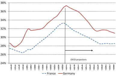
We select two different demographic structures existing in two countries with relatively com-parable economic structures, namely, France and Germany. Figure 1 displays the dynamics over time of the fraction of the population that is aged 40-65 in France and in Germany. It shows that
8Accordingly, the price of a barel of Brent is 157$
2010 in 2025; the end-use price of natural gas for household reaches 75€2010/MWh in 2025; the real supply price of a ton of coal is 99€2010in 2025.
9This increase is linear from 1,0% per year in 2010 to 2,0% per year from 2020 on. 1 0Defined here as encompassing hydroelectricity, wind and PV .
24% 26% 28% 30% 32% 34% 36% 38% 1 9 7 0 1 9 7 3 1 9 7 6 1 9 7 9 1 9 8 2 1 9 8 5 1 9 8 8 1 9 9 1 1 9 9 4 1 9 9 7 2 0 0 0 2 0 0 3 2 0 0 6 2 0 0 9 2 0 1 2 2 0 1 5 2 0 1 8 2 0 2 1 2 0 2 4 2 0 2 7 2 0 3 0 2 0 3 3 2 0 3 6 2 0 3 9 2 0 4 2 2 0 4 5 2 0 4 8 France Germany OECD projections
Figure 1: Percentage of the population that is aged between 40 and 65
the demographic structure has been different in France and Germany for decades, with Germany having on average an older population of working age. In the OECD projections, the fraction of the population that is aged 40-65 will remain higher in Germany than in France in the next decades.11
In line with life-cycle theory, this group of cohorts saves more than other demographic groups in the model, in absolute as well as in relative terms.
... higher lump-sum public expenditures
... lower proportional, direct income taxes Germany Scenario DEU EXP Scenario DEU TAX
France Scenario FRA EXP Scenario FRA TAX Carbon tax redistributed through…
Figure 2: Main scenarios simulated in the model
Such a setting allows for measuring the link between the demographic structure and the mag-nitude of the second dividend. By construction, in a dynamic GE model, all the variables interact with one another. The only way to isolate the influence of one variable (e.g., the demographic structure) on another (e.g., the second dividend) in the intertemporal, general equilibrium consists in running two scenarios where the only difference is the first variable (i.e., demographic structure). By definition, the second dividend on German data is measured by computing each year the difference between the level of GDP in scenario DEU TAX and scenario DEU EXP. This difference
is not directly related with the effect of the demographic structure on the GDP level.12 Indeed, it is
computed from the results of two scenarios that rely on the same demographic structure. Let’s call this difference A. In order to measure the influence of the demographic structure on the size of the second dividend, an intermediary step is necessary. We run two additional scenarios consisting in computing scenario DEU EXP and scenario DEU TAX but using French demographic data, instead of German demographic data as in the previous step. The difference each year between the level of GDP in scenario DEU TAX with French demographic data and the level of GDP in scenario DEU EXP with French demographic data is the second dividend in Germany with a different (i.e., non German) demographic structure. This difference is not directly related with the effect of the demographic structure on the GDP level because it is computed from the results of two scenarios that rely on the same demographic structure (in this case, a French one). Let’s call this difference B.
The difference between A and B as defined above is the effect of the demographic structure on the second dividend. It is still not directly related with the effect of the demographic structure on the GDP level since it is computed as a difference of two differences that are not directly related with the effect of the demographic structure on the GDP level since each is computed from the results of two scenarios that rely on the same demographic structure.13
This method can also be presented intuitively. The dynamics of the model is driven by a) demographics, b) reforms in the sector of energy, c) fiscal policies, d) world energy prices, and e) optimal responses of economic agents to price signals (i.e., interest rate, wage, energy prices). The modelling of factors d) and e) is identical in all scenarios for both countries. The modelling of factor c) is almost identical here in Germany and France. Factor b) is somewhat different whether the model is parameterised on French or German data. Factor a) - e.g., demographics - is different between the two countries. Accordingly, the difference between the magnitude of the second dividend in Germany and in France should mainly stem in the model either from demographic differences, or from differences between energy policies, with an intuition that the former effect dominates the latter. In this context, if the difference between DEU EXP with French demographics and DEU TAX with French demographics is close to the second dividend in France (i.e., FRA EXP - FRA TAX), then most of the difference between Germany and France as concerns the magnitude of the second dividend mirrors demographic factors. On the other hand, if the difference between
1 2By "directly", we mean before macroeconomic feedback effects.
1 3Another equivalent method could have been used, yielding the same results. As a first step, let’s compute the difference between the level of GDP in scenario DEU EXP and scenario FRA EXP. This difference measures the effect on the level of GDP of changing the demographic structure (in scenarios where the environmental tax is recycled through higher lump-sum spending). This difference is directly related with the effect of the demographic structure on the GDP level because it is computed from the results of two scenarios that rely on two different demographic structures. Let’s call this difference C. Second step: compute the difference between the level of GDP in scenario DEU TAX and scenario FRA TAX. This difference measures the effect on the level of GDP of changing the demographic structure, in scenarios where the environmental tax is recycled through lower distorsive taxes). This difference is directly related with the effect of the demographic structure on the GDP level because it is computed from the results of two scenarios that rely on two different demographic structures. Let’s call this difference D. The difference between C and D measures the effect of the demographic structure on the second dividend. Indeed, it is still not directly related with the effect of the demographic structure on the GDP level since it is computed as a difference of two differences, each of them being computed from the results of two scenarios incorporating the same change in the demographic structure.
In this empirical model, the effect of the demographic structure on the level of GDP and the effect of the demo-graphic structure on the second dividend are easily distinguishable: the former is quantitatively significantily larger than the latter.
DEU EXP with French demographics and DEU TAX with French demographics is close to the second dividend in Germany (i.e., DEU EXP - FRA DEU), then the conclusion would be that the effects of demographic factors on the magnitude of the second dividend remain subdued.
3
Results
We present some aggregate results of the scenarios before going directly and in more detail to the implications on GDP growth.
3.1
Aggregate effects
• in the scenarios on German data, the energy transition policy triggers a rise of renewables as a share in the production of electricity from the current levels to 35% in 2020, 50% in 2030 and 65% in 2040. PV, onshore and offshore wind produce overall 155TWh in 2020 in the model. This is close to the official target of 146TWh, which does not take account of GE effects (whereas the model does). The downward effect on wholesale prices in the model amounts to -29€/MWh in 2030. The associated consequences are sizeable for feed-in tariffs (from 40€/MWh in 2013 in the model to 70€/MWh in 2030) as well as for electric network costs (from 17€/MWh in 2013 to 55€/MWh in 2030). Overall, average retail prices of electricity rise by 76% in 2030 in real terms as compared to their level in 2008. The total weighted end-use price of energy surges from 2008 to 2030 (+55% in real terms), mirroring partly the effect of the implementation of the carbon tax from 2015 onwards. The share of total renewables in the total final consumption of energy is 27% in 2025 in the model. German publicly announced targets imply a rise in efficiency gains from 1,5% per year over the recent past to around 2,2% per year in the future.14 The total demand for energy declines over the next decades (by close to -20% up to 2030). As concerns public finances, in case the carbon tax is recycled through higher public lump-sum expenditures, these spendings increase from 18,0% of gross disposable income to 18,6%, ceteris paribus and in the short-run. When the carbon is recycled through a lower proportional income tax financing the lump sum public expenditures regime, the rate of the tax declines from 18% to 17,4% ceteris paribus and in the short-run. Eventually, since German demography is ageing relatively quickly, the capital per unit of efficient labour rises gradually in the next decades.
• in the scenarios on French data, a carbon tax is implemented from 2015 onwards in the model, with the same characteristics as in the model on German data. The associated annual public income reaches 17bn€2010in 2030. The price of CO2 in the EU-ETS is supposed to be indexed to
the rate of the carbon tax and increases thus sizeably. The main peaker on the electricity market remains coal up to the late 2020’s. The end-use price of electricity for households increases by 80% in real terms between 2010 and 2030, mainly as a consequence of the impact of the development of renewables on taxes and network costs, and the implementation of the carbon tax. The total weighted end-use price of energy displays a very strong upward trend (+70% in real terms from 2010 to 2030). In this context, the total demand for energy remains sluggish over the next decades.
Production price of natural gas ($/MBTu) Production price of oil ($/barel) Production price of coal (€/t)
Rate of the carbon tax on oil products and natural gas (€/t) Amount of the carbon tax if created in 2015 (bn€) Impact of wind and PV on average market price (€/MWh) Production market price of electricity (€/MWh)(incl. effect of renewables)(*)
Impact of wind and PV on grid-level system costs (€/MWh) Price of electricity - retail - households (€/MWh) Price of electricity - industry (€/MWh)
Total weighted end-use price of energy in the model (1989=100) Demand for energy (1989=100)
Fraction of renewables in the energy mix (incl.hydro, wind, PV)(%)
Rate of the social contribution to the pension regime (%) Replacement rate of the pension regime (%)
Average effective age of retirement (years)
Rate of the social contribution to the health regime (%) Public debt (% GDP)
2009 2040 2009 2040 2009 2040 2009 2040
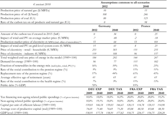
Tax financing non-ageing related public spendings (% of gross income) 18,0% 18,0% 18,0% 16,9% 20,0% 20,0% 20,0% 19,2% Non-ageing related public spendings (% of gross income) 18,0% 19,1% 18,0% 18,0% 20,0% 20,8% 20,0% 20,0% Capital per unit of efficient labour (1989=100) 139,03 146,18 139,03 146,65 120,13 114,78 120,13 114,90 Average cost of productive capital (real)(1989=100) 74,69 71,40 74,69 71,20 85,08 88,58 85,08 88,50 GDP level (1989=100) 138,91 177,78 138,91 177,82 154,75 224,17 154,75 224,24 78% 95% 61 65 61 65 7% 9% 11% 13% 16% 39% 15% 25% 9% 9% 11% 11% 57% 44% 61% 45% 184 292 144 247 96 77 115 102 8 131 96 23 235 157 15 253 119 61 383 188 101 2012 2040 10 108 80 0 15 246 123 98 55 -40 64 -2 53 0 34 0 25 -7 -18
Assumptions common to all scenarios
Germany France 2012 2040 2012 2040
(*) In the model, the dynamics of the future market price of production of electricity diverges between Germany and France because a) France will keep using nuclear energy for producing electricity, the cost of which will increase for safety reasons, whereas Germany will shut down its nuclear facilities in the next decade; b) the strong development of renewables will weigh far more significantly of the market production price of electricity in Germany than in France. However, German private agent face much higher future retail prices of electricity than in France in the model, in line with rising system costs and feed-in tariffs related with renewables.
DEU EXP DEU TAX FRA EXP FRA TAX
€ constant 2010
Figure 3: Aggregate results
Taxation of carbon magnifies the effects on energy demand stemming from high prices of fossil fuels on world markets, along with the impact of accelerating gains in energy efficiency. The energy mix displays a rise of the renewable sources of energy15, from 12% of total demand in 2010 to 23%
in 2025. Capital per unit of efficient labour unit declines slowly over the next decades, mirroring among other factors the effects of demographics that is relatively more favourable in France than in Germany.
3.2
Implications on growth dynamics
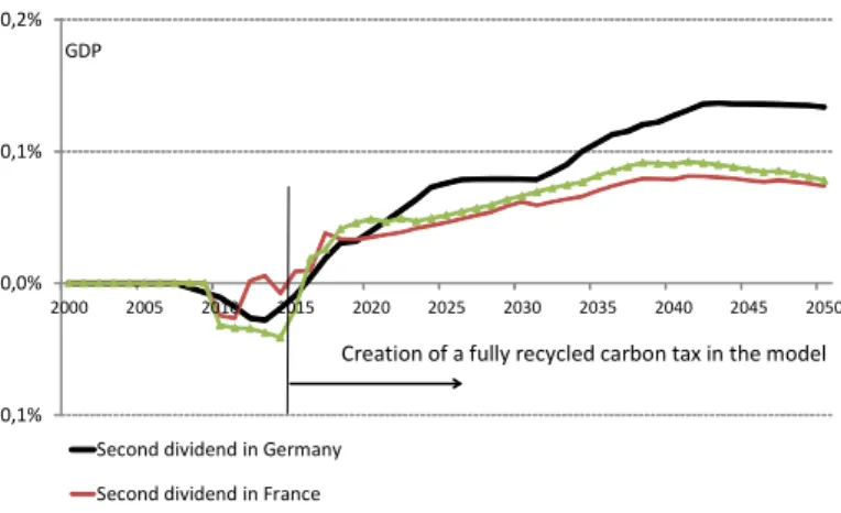
Figure 4 displays the results obtained in the model as concerns growth dynamics. Several results emerge.16
1 5This increase mirrors both the effects of the energy transition policy and the increase of the prices of fossil fuels. 1 6In Figure 3, the GDP appears somewhat lower in the early 2010’s in the scenarios with a recycling of the carbon tax through lower taxes than in the scenarios with a recycling of the carbon tax through higher lump-sum public expenditures. This mirrors different modelling assumptions that do not have far reaching economic implications nor significance. The reform consisting in recycling the carbon tax through lower taxes rather than higher lump-sum public expenditures is announced in 2010 and implemented in 2015 in the model (by assumption). This triggers
-0,1% 0,0% 0,1% 0,2%
2000 2005 2010 2015 2020 2025 2030 2035 2040 2045 2050
Second dividend in Germany Second dividend in France
Second dividend in Germany with another (i.e., French) demographic structure
Creation of a fully recycled carbon tax in the model
GDP
Figure 4: Impact on the GDP level of a second dividend
Result 1: The second dividend is positive in the model since GDP is fostered when the carbon tax is recycled through lower proportional income taxes instead of higher lump-sum public expenditures.
In our model this is mainly because lessening the proportional tax amounts, in absolute terms, to distributing more revenues to cohorts receiving higher wages. These cohorts receiving on average a higher gross labour income are relatively older working cohorts, which are more productive in the model than the younger ones. In line with the life-cycle theory, the saving rate of aged working cohorts is also higher than the one of younger working cohorts. Overall, capital supply is higher in scenario DEU TAX than in scenario DEU EXP (with the same result appying also on French data) and this stems from demographic factors.
The dynamics of the labour supply and of the optimal average working time is more complex in the model and mirrors different effects (a direct demographic effect, a capital-deepening effect, a structural productivity effect, a tax distorsive effect, a public spending effect and a direct carbon tax effect) of which the net effect is close to zero in the model. These effects stem from the first order intratemporal condition for a working individual, which can be written as 1 − ℓ∗
t,a = c∗
t,a(κξHa−1)
[wtεa(1−τt,D−τt,P−τt,H−τt,N A)+dt,NA−dt,energy]ξ (where 1 − ℓ ∗
t,ais optimal leisure and ξ > 0). A direct
demographic effect fosters the gross wage (wt) because labour is scarcier in an ageing society, thus
its relative price increases. Accordingly, leisure diminishes, ceteris paribus. A capital deepening effect weighs on consumption in the model (c∗
t,a) because it lessens the interest rate and the first
order intertemporal condition shows that this has a decelerating effect on consumption, thus on optimal leisure, ceteris paribus. A structural productivity effect is related with the positive impact of ageing on εa: since the average working individual ages in the model, its productivity increases
over time and this lessens, ceteris paribus, the optimal level of leisure. A distorsive effect of taxes on labour supply ((1 − τt,P− τt,H− τt,NA)ξwith ξ > 0) captures the positive influence on leisure
higher saving which lessens somewhat the GDP level in the short run but, through stronger future capital deepening, enhances growth after some years.
of a rise in tax rates (or, equivalently, the positive influence on working time of lower tax rates). A public lump-sum spending effect flows through parameter (dt,NA). Eventually, a direct carbon tax
effect appears through the amount of expenditures in energy (dt,energy) which is influenced by the
introduction of a carbon tax (with an upward price effect partially offset by a downward volume effect, the net effect being positive on optimal leisure). In scenarios where the carbon tax is recycled through higher lump-sum public expenditures (dt,NA), there is no distorsive effect of a change in
the tax rates, but a favourable public spending effect on optimal leisure as well as on the level of consumption (the latter lessening the above quoted capital deepening effect).
Overall, since capital supply is higher in scenario DEU TAX than in scenario DEU EXP, and since labour supply remains practically identical in both scenarios, then growth in scenario DEU TAX is slightly higher than growth in scenario DEU EXP. The same features qualitatively apply to the model parameterized on French data. Qed.
Result 2: the macroeconomic magnitude of the second dividend remains subdued in the model. In the long-run, around 2050, the macroeconomic magnitude of the second dividend is expected to be around +0,1%. This is in line with the conventional wisdom of the "elephant and rabbit" tale in energy economics (Hogan and Manne, 1977) according to which the size of the energy sector in the economy bares it to entail very sizeable effects on growth. We only remind here that what was accurate when Hogan and Manne wrote their article, might be less so in our post-financial crises era characterized by very limited growth.
Result 3 (main result): the dynamic aggregate second dividend is relatively higher in a country with a relatively older working population.
This can be directly observed on Figure 4. As said above, the difference between the magnitude of the second dividend in Germany and in France can stem in the model either from demographic differences, or from differences between energy policies. Figure 4 displays the macroeconomic effect of the second dividend in scenarios paramterised on Germand data except for demographics where French data have been used. It shows that the difference between the dynamics of GDP in the DEU EXP scenario with French demographics and in the DEU TAX scenario with French demographics is close to the macroeconomic influence of the second dividend measured on French data (i.e., FRA EXP - FRA TAX). Accordingly, most of the difference between Germany and France as concerns the magnitude of the second dividend mirrors demographic factors.
Intuitively, when the demographic structure is relatively more concentrated on cohorts with higher saving rate, a policy distributing more income to these cohorts entail a relatively stronger effect on capital supply. The model suggests that the impact on labour supply remains limited (see above). Thus, the more concentrated the demographic structure on cohorts with a high saving rate, the higher the macroeconomic influence of the second dividend related with an environmental tax reform.
Result 4: the magnitude of the second dividend remains practically unaffected by alternative assumptions as concerns the dynamics of future energy prices on world markets.
Even with an oil price 30% lower in 2025 than in the scenarios presented above, the size of the second dividend would not be sizeably modified.
3.3
Intergenerational redistributive effects of a dynamic aggregate
sec-ond dividend
3.3.1 Effects on future annual welfare of each cohort
A first detailed analysis of the cohorts loosing or gaining in different scenarios is possible using Lexis surfaces (Figures 5 and 6). A Lexis surface represents in 3 dimensions the level of a variable associated with a cohort of a given age at a given year. The variable considered here is the gain (or loss) of annual welfare of a cohort aged a in a given year t and in a scenario where the carbon tax is recycled through lower proportional income tax compared to the baseline scenario where the carbon tax is recycled through higher lump-sum public spending. Annual welfare refers here to the instantaneous utility function of a private agent in the model, and thus depends on the level of consumption and optimal leisure. Before the announcement of a reform package in 2010, annual current welfare of one cohort is by assumption equal in both scenarios. Graphically, this involves a flat portion in the Lexis surface, at value 0. From 2010 onwards, the deformations of the Lexis surfaces mirror the influence of mechanisms of intergenerational redistribution of the second dividend, as measured by its influence on current welfare.
Result 5: the second dividend displays pro-youth intergenerational redistributive features in the model.
Figure 5 and 6 display the Lexis surface for current welfare at each year for each cohort in the model on German (resp., French) data, in the scenario where the carbon tax is recycled through lower proportional income tax compared to the baseline scenario where the carbon tax is recycled through higher lump-sum public spending. Thus it materializes the intergenerational effects of the second dividend in Germany (resp., France) in the model.
As shown in Figures 5 and 6, it weighs on the future annual welfare of currently relatively aged working cohorts. It simultaneously fosters the future annual wellbeing of currently relatively young working cohorts, and of future generations. Before explaining the two main mechanisms involved for this result, it may be useful to remind here that annual welfare in the model depends on the optimal consumption and leisure paths defined by perfectly anticipating households over their whole life-cycle, and not on their current income.
In this context, result 5 flows mainly from the joint influence of a distorsive effect (enshrined in the intratemporal arbitrage between work and leisure) and a capital deepening effect (stemming from the intertemporal arbitrages between consumption and saving):
• the distorsive effect refers to the positive influence due to lower income taxes on optimal working time, thus on income and wellbeing. This effect does not exist for higher lump-sum public spending. The younger the cohort, the longer the effect over its whole life-cycle, the stronger the positive impact on income and wellbeing.
• the capital deepening effect flows from the conditions of the consumption/saving arbitrage. Recycling the revenue of the carbon tax through lower direct taxes increases relatively more the income of the relatively numerous aged working cohorts, in absolute terms, and their savings as well (as seen in result 1 above). On the aggregate scale, this entails a higher capital deepening than
2000 2010 2020 2030 -0,2% -0,1% 0,0% 0,1% 0,2% 0,3% 0,4% 20 30 40 50 60 70 AGE YEAR
Figure 5: Effect on annual welfare of recycling a carbon tax through lower proportional income taxes instead of higher lump-sum public spending (in Germany, in %)
2000 2010 2020 2030 -0,2% -0,1% 0,0% 0,1% 0,2% 0,3% 0,4% 20 30 40 50 60 70 YEAR AGE
Figure 6: Effect on annual welfare of recycling a carbon tax through lower proportional income taxes instead of higher lump-sum public spending (in France, in %)
if the carbon tax had been recycled through higher lump-sum public expenditures. This weighs relatively more on the optimal consumption path of older cohorts in the model because it depresses the yield of the saving of these relatively numerous cohorts which have accumulated (much) more capital than younger cohorts when the public policy is announced in the model. Younger cohorts suffers relatively less from this effect since their accumulated capital is lower (and even negative at the beginning of the life-cycle) and since its influence will materialize for them in 2 or 3 decades in the future and will be discounted accordingly in the definition of their optimal consumption and leisure paths.17
• overall, the capital-deepening effect of the second dividend weighs relatively more on the wellbeing of the aged working cohorts (i.e., the baby-boomers) and the distorsive effect of the second dividend bolsters relatively more the wellbeing of the youths (i.e., the children of the baby-boomers). What the model additionnally suggests is that the distorsive effect dominates the capital-deepening effect for the young working cohorts (since the effect of the second dividend is positive for them as shown in Figures 5 and 6), and vice-versa for the aged working cohorts (since the effect of the second dividend is negative for them as shown in Figures 5 and 6).
Result 6: the magnitude of the pro-youth intergenerational redistributive properties of the second dividend is influenced by the demographic structure.
As shown in Figures 5 and 6, it is higher in Germany than in France. Result 3 suggests that this stems mainly from demographic factors. The demographic structure does not directly influence the intratemporal arbitrage of the households and hence the distorsive effect of the second dividend. However, it does impact directly the capital intensity of the economy, the capital yield and hence the intertemporal arbitrage of the cohorts.
Germany will experience (and is already currently experiencing) more capital deepening than France because of less favourable demographics and a relatively scarcier labour input in its produc-tion funcproduc-tion. This involves a slightly increasing capital intensity over the next decades in Germany while the capital per efficient unit of labour may stabilise or even slightly decline in the future for France. These dynamics in turn account for a capital yield that decline in Germany up to the late 2020’s in the model, before starting to increase again; while the capital yield would remain broadly stable in France over the same period. Consequently, the capital deepening effect of the second div-idend will be stronger for German aged working cohorts (i.e., baby-boomers) than for their French counterparts in the model. This explains that the wellbeing loss related with the second dividend for aged working cohorts is higher in Germany than in France, as displayed in Figure 5 and 6.
By contrast, the younger working cohorts and the future generations will benefit from the rise in the capital long-run equilibrium yield in Germany from the 2030’s onwards. Accordingly, the capital deepening effect of the second dividend will be lower for German young working cohorts (i.e., baby-boomers) and future generations than for their French counterparts in the model. This explains that the wellbeing gains related with the second dividend for young working cohorts and future generations is higher in Germany than in France, as shown in Figure 4 and 5.
1 7These intergenerational redistributive effects are robust to different assumptions as concerns future prices of fossil fuels on world market.
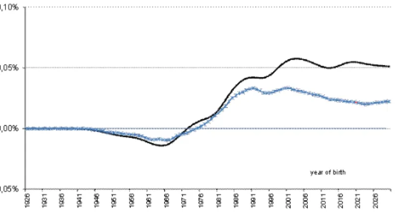
Figure 7: Effects on the intertemporal welfare of recycling a carbon tax through lower proportional income tax instead of higher lump-sum public spending
3.3.2 Effects on intertemporal welfare of private agents
Computing the intertemporal welfare of each cohort over its whole lifetime allows for precising and completing the above analysis of intergenerational redistributive effects. Figure 7 displays, on German and French data, the effects on intertemporal welfare of each cohort of a scenario where the carbon tax is recycled through lower proportional income tax compared to the baseline scenario where the carbon tax is recycled through higher lump-sum public spending.
Result 7: The second dividend fosters the intertemporal wellbeing of young active cohorts and future generations, while weighing slightly on the intertemporal wellbeing of currently aged working cohorts.
This result is in line with result 5; however it additionnally provides with a quantitative as-sessment, from an intertemporal point of view, of the magnitude of the redistributive mechanisms involved by the second dividend.
Result 8: The magnitude of the intertemporal redistributive effect of the second dividend is related with the demographic structure.
This appears directly on Figure 6 and provides a quantitative assessment, from an intertemporal perspective, of the mechanisms involved in result 5. The more concentrated the demographic struc-ture on aged working cohorts, the higher the redistributive effects of a second dividend stemming from recycling a carbon tax with lower proportional income tax rather than higher lump-sum public expenditures.
Result 9: As far as the intertemporal wellbeing of the cohorts is concerned, the second divi-dend of recycling a carbon tax through lower proportional income tax rather than lump-sum public expenditures is not far from being a Pareto-improving policy.
Again, this appears in Figure 7 which shows that the negative effect of the second dividend on the intertemporal wellbeing of aged working cohorts remains subdued, whereas its favourable effects on the intertemporal wellfare of younger working cohorts and future generations is relatively more sizeable.
4
Conclusion and policy implications
This paper assesses the empirical, aggregate, intertemporal impact of the demographic structure on the magnitude of the "second dividend" associated with an environmental tax. The main result is that the older the working population, the higher the second dividend. The intuition is that when the demographic structure is relatively more concentrated on cohorts with higher income and saving rate, then a policy redistributing more income to these cohorts entails a relatively stronger effect on capital supply. Results also suggest that the second dividend displays pro-youth intergenerational redistributive features. This result flows mainly from the joint influence of a distorsive effect and a capital deepening effect. The latter weighs relatively more on the wellbeing of the aged working cohorts while the former bolsters relatively more the wellbeing of the young cohorts. The more concentrated the demographic structure on aged working cohorts, the higher the redistributive, pro-young effect of a second dividend.
These results have direct policy implications. If some government seeks to increase the second dividend of an environmental tax and its pro-youth redistributive properties, then the magnitude of this tax reform should be relatively more important in countries with relatively younger working populations.
This analysis shows that demographic structures can play a significant role in energy economics and policies. Overlapping generation frameworks enshrined in EG modeling are well suited for studying such issues.
A
Description of the GE-OLG model
This CGE model displays an endogenously generated GDP with exogenous energy prices influ-encing macroeconomic dynamics, which in turn affect the level of total energy demand and the future energy mix. GE-OLG models combine in a single framework the main features of GE models (Arrow and Debreu, 1954), Solow-type growth models (Solow, 1956), life-cycle models (Modigliani and Brumberg, 1964) and OLG models (Samuelson, 1958). The development of applied GE-OLG models, using empirical data, owes much to Auerbach and Kotlikoff (1987). This GE model includes a detailed overlapping generations framework so as to analyse, in a dynamic setting, the intergen-erational redistributive effects of energy and fiscal reforms, and to take account of demographic dynamics on the economic equilibrium.18
A.1
The Energy sector
A.1.1 Energy prices
End-use prices of natural gas, oil products and coal (q1,t, q2,t, q3,t) The end-use prices of
natural gas, oil products and coal (qi,t, i ∈ {1; 2; 3}) are computed as weighted averages of prices of
different sub-categories of energy products: ∀i ∈ {1; 2; 3} , qi,t= n j=1
ai,j,tqi,j,t. qi,j,t stands for the
real price of the product j of energy i at year t. For natural gas (i = 1), two sub-categories j are modeled: the end-use price of natural gas for households (j = 1) and the end-use price of natural gas for industry (j = 2). For oil products (i = 2), three sub-categories j are modeled: the end-use price of automotive diesel fuel (j = 1), the end-use price of light fuel oil (j = 2) and the end-use price of premium unleaded 95 RON (j = 3). For coal (i = 3), two sub-categories j are modeled: the end-use price of steam coal (j = 1) and the end-use price of coking coal (j = 2). This hierarchy of energy products covers a great part of the energy demand for fossil fuels. The ai,j,t’s weighting
coefficients are computed using observable data of demand for past periods. For future periods, they are frozen to their level in the latest published data available: whereas the model takes account of interfuel substitution effects (cf. infra), it does not model possible substitution effects between sub-categories of energy products (for which data about elasticities are not easily available).
The end-use prices of sub-categories of natural gas, oil or coal products (qi,j,t) are in turn
computed by summing a real supply price with transport/distribution/refining costs and taxes: ∀i ∈ {1; 2; 3} , ∀j, qi,j,t= qi,j,t,s+ qi,j,t,c+ qi,j,t,τ
1 8In line with most of the literature on dynamic GE-OLG models, the model used here does not account explicitly for effects stemming from the external side of the economy. First, the main question that is adressed here is: what optimal choice should the social planner do as concerns energy and fiscal transition so as to maximize long-run growth and minimize intergenerational redistributive effects? Accounting for external linkages would not modify substantially the answer to this question. It would smooth the dynamics of the variables but only to a limited extent. Home bias (the “Feldstein-Horioka puzzle”), exchange rate risks, financial systemic risk and the fact that many countries in the world are also ageing and thus competing for the same limited pool of capital all suggest that the possible overestimation of the impact of ageing on capital markets due to the closed economy assumption is small.
• qi,j,t,s stands for the real supply price at year t of the product j of energy i. This real
price is computed as a weighted average of real import costs and real production prices: ∀i ∈ {1; 2; 3} , ∀j, qi,j,t,s = [Mi,j,tmi,j,t+ Pi,j,tpi,j,t] / [Mi,j,t+ Pi,j,t] where Mi,j,t stands for imports in
volume of the product j of energy i at year t ; mi,j,t stands for imports costs of the product j of
energy i at year t ; Pi,j,t stands for national production, in volume, of the product j of energy i
at year t ; pi,j,t stands for production costs of national production of the product j of energy i at
year t. The weights Mi,j,t and Pi,j,t are computed using OECD/IEA databases for past periods,
and frozen to their latest known level for future periods.
• qi,j,t,c stands for the cost of transport and distribution and/or refinery for the different
energy products for natural gas, oil and coal. More precisely, q1,1,t,c stands for the cost of transport
and distribution of natural gas for households in year t; q1,2,t,c stands for the cost of transport
of natural gas for industry in year t; q2,1,t,c , q2,2,t,c and q2,3,t,c stand respectively for the cost of
refining and distribution for automotive diesel fuel, light fuel oil and premium unleaded 95 RON in year t; q3,1,t,cand q3,2,t,c stand respectively for the transport cost of steam coal and coking in year
t. The qi,j,t,c’s are calculated as the difference between the observed end-use prices excluding taxes
by category of products (as provided by OECD/IEA databases) and the supply prices (the qi,j,t,s’s)
as computed above. For future periods, each qi,j,t,c’s is computed as a moving average over the 10
preceding years before year t.
• qi,j,t,τ stands for the amount, in real terms, of taxes paid by an end-user of a product j of
energy i at year t. For past periods, these data are provided by OECD/IEA databases. They include VAT, excise taxes, and other taxes: qi,j,t,τ = V ATi,j,t+ Excisi,j,t+ othersi,j,t+ carbon taxi,j,t. For
future periods, the rate of V ATi,j,tand othersi,j,tare computed as a moving average over the latest
10 years before year t, and the absolute real level of Excisi,j,tis computed as a moving average over
the latest 10 years before year t. For future periods, depending on the reform scenario considered, qi,j,t,τ can also include a carbon tax (carbon taxi,j,t) which is computed by applying a tax rate to
the carbon contained in one unit of volume of product j of energy i.
Prices of electricity (q4,t) The real end-use price of electricity is computed as a weighted average
of prices of electricity for households and industry (i = 4); q4,t= 2 j=1
a4,j,tq4,j,t. q4,j,tstands for the
end-use real price, at year t , of the product j of electricity. Two sub-categories j are modeled: the end-use price of electricity for households (j = 1) and the end-use price of electricity for industry (j = 2). The a4,j,t’s weighting coefficients are computed using observable data of demand for past
periods, and frozen to their level in the latest published data available for future periods. Real end-use prices of electricity are computed by adding network costs of transport and distribution (q4,j,t,c)
and differents taxes (VAT, excise, tax financing feed-in tariffs for renewables, carbon tax...)(q4,j,t,τ)
to an endogenously generated (structural) wholesale market price of production of electricity (q4,t,s):
(i = 4); ∀j, q4,j,t= q4,t,s+ q4,j,t,c+ q4,j,t,τ
Wholesale structural market price of production of electricity (q4,t,s) The wholesale
market price of production of electricity (q4,t,s) is computed from an endogenous average peak price
of electricity and a peak/offpeak spread: ∀j, q4,t,s= (qel,peak,t+spread2peak,t∗qel,peak,t). The parameter
The peak market price of production of electricity (qel,peak,t) derives from costs of production of
electricity among different technologies, weighted by the rates of marginality in the electric system of each production technology: qel,peak,t =
9 x=1
ξel,x,t̺el,x,t,prod (1+ξel,import,t) 9
x=1ξel,x,t +ξel,import,t+̟f atal,t
. The costs of producing electricity (̺el,x,t,prod) are computed for 9 different technologies x: coal (x = 1), natural gas (x = 2), oil (x = 3), nuclear (x = 4), hydroelectricity (x = 5), onshore wind (x = 6), offshore wind (x = 7), solar photovoltaïc (x = 8), and biomass (x = 9). The ξel,x,t’s stand for the rates of marginality in the electric system of the producer of electricity using technology x
Cost of production of electricity among different technologies (̺el,x,t,prod) Following, for instance, Magné, Kypreos and Turton (2010), each ̺el,x,t,prodis computed as the sum of variable costs (i.e., fuel costs and operational costs) and fixed (i.e., investment) costs of producing electricity: ∀x, ̺el,x,t,prod= ̺el,x,t,f uel+̺co2 price,t∗̺el,x,t,co2em
̺el,x,t,therm + ̺el,x,t,ops +̺el,x,t,f ixedwhere ̺el,x,t,f uelstands
for the fuel costs for technology x (either coal, oil, natural gas, uranium, water, biomass for costly fuel, or wind and sun for costless fuels) measured in €/MWh; ̺el,x,t,therm stands for thermal efficiency (in %). CO2 costs are measured by the exogenous price of CO2 on the market for quotas (EU ETS) (̺co2 price,t, in €/ton), as applied to technology x characterised by an emission factor ̺el,x,t,co2em expressed in t/MWh; ̺el,x,t,opsstands for operational and maintenance variable costs (in €/MWh). Fixed costs ̺el,x,t,f ixed are expressed in €/MWh and computed according to the following annuity formula: ∀x, ̺el,x,t,f ixed = ̺el,x,t,inv
1+̺el,x,t,prodloss
1+̺el,x,t,learning̺el,x,t,cap c
(1−(1+̺el,x,t,cap c)−̺el,x,t,lif e)̺el,x,t,util
. ̺el,x,t,inv corresponds to overnight cost of investment (expressed in €/MW); ̺el,4,t,prodloss is the rate of productivity loss due to increased safety in the nuclear industry ; ̺el,x,t,learning is the learning rate for renewables; ̺el,x,t,cap c stands for the cost of capital (̺el,x,t,cap c= 10%); ̺el,x,t,lif e the average lifetime of the facility (in years) depending of the technology used; ̺el,x,t,util the utilisation rate of the facility (in hours). All these parameters are exogenous and found mainly in IEA and/or NEA databases.
Rates of marginality (ξel,x,t) and main peaker between coal firing and natural gas firing (ξel,1,t and ξel,2,t) The rates of marginality are the fraction of the year during which a producer of electricity is the marginal producer, thus determining the market price during this period. These rates are exogenous in the model. They are computed in France by the French Energy Regulation Authority and/or by operators in the electric sector in France and Germany. For future periods, the model uses the 2010 values which are frozen onwards.19
The computation of the future values for ξel,1,tand ξel,2,tin the model stems from an endogenous determination of the main peaker, either coal firing or natural gas firing. The model computes, for each year t > 2012, the clean dark spread and the clean dark spread. These are mainly influenced by CO2 prices (̺co2 price,t), respective emission factors (̺co2 price,tand ̺el,2,t,co2em) and fuel costs (̺el,x,1,f uel and ̺el,x,2,f uel). Each year t > 2012, if the difference between the clean spark spread
1 9Accordingly, the formula used for computing (q
elec,peak,t) assumes that the energy mix of imports is the same as the domestic energy mix.