Complexity reduction methods applied to the rapid solution to multi-trace boundary integral formulations.

(1)

HAL Id: tel-02004298

https://tel.archives-ouvertes.fr/tel-02004298

Submitted on 1 Feb 2019

HAL is a multi-disciplinary open access

archive for the deposit and dissemination of sci-entific research documents, whether they are pub-lished or not. The documents may come from teaching and research institutions in France or abroad, or from public or private research centers.

L’archive ouverte pluridisciplinaire HAL, est destinée au dépôt et à la diffusion de documents scientifiques de niveau recherche, publiés ou non, émanant des établissements d’enseignement et de recherche français ou étrangers, des laboratoires publics ou privés.

Complexity reduction methods applied to the rapid

solution to multi-trace boundary integral formulations.

Alan Obregón

To cite this version:

Alan Obregón. Complexity reduction methods applied to the rapid solution to multi-trace bound-ary integral formulations.. Mathematics [math]. Sorbonne University UPMC, 2018. English. �tel-02004298�

(2)

Thèse présentée pour obtenir le grade de

DOCTEUR DE L’UNIVERSITÉ SORBONNE

Spécialité : Mathématiques appliquées

par

Alan Ayala Obregón

Complexity reduction methods applied to the rapid

solution to multi-trace boundary integral

formulations

soutenue le 16 novembre 2018 devant le jury composé de :

Bruno Després Sorbonne Université - LJLL président du jury

Patrick Ciarlet ENSTA, ParisTech rapporteur

François Alouges Ecole Polytechnique – CMAP rapporteur

Eric Darrigrand Université de Rennes 1 examinateur

Laura Grigori Sorbonne Université - INRIA Paris directeur de thèse Xavier Claeys Sorbonne Université - INRIA Paris directeur de thèse

(3)

Abstract

The objective of this thesis is to provide complexity reduction techniques for the solution of Boundary Integral Equations (BIE). In particular, we focus on BIE arising from the modeling of acoustic and elec-tromagnetic problems via Boundary Element Methods (BEM). Our approach consists in using the local multi-trace formulation which is friendly to operator preconditioning. We find a closed form inverse of the local multi-trace operator for a particular scattering model problem and then we propose this inverse operator for preconditioning general scattering problems. We numerically show that this pre-conditioner is efficient and accelerates the solution of the linear system obtained from the discretization of the continuous problem. We also show that the local multi-trace formulation is stable for Maxwell equations posed on a particular domain configuration.

For general problems where BEM are applied, we propose to use the framework of hierarchical ma-trices, which are constructed using cluster trees and allow to represent the original matrix in such a way that submatrices that admit low-rank approximations (admissible blocks) are well identified. We intro-duce a technique called geometric sampling which uses cluster trees to sample row and column indices allowing to create accurate linear-time CUR algorithms for the compression and matrix-vector product acceleration of admissible matrix blocks, and which are oriented to develop parallel communication-avoiding algorithms.

For the general framework of low-rank approximations, we study widely used techniques based on QR factorizations and subspace iteration methods; for the former we provide new bounds for the classical column pivoting and general pivoting strategies, and for the later we solve an open question in the literature consisting in proving that the approximation of singular vectors exponentially converges. Finally, we propose a technique called affine low-rank approximation intended to increase the accu-racy of classical low-rank approximation methods, in particular for those based on QR and subspace iteration.

(4)

Résumé

L’objectif de cette thèse est de fournir des techniques de réduction de complexité pour la solution des équations intégrales de frontière (BIE). En particulier, nous sommes intéressés par les BIE issues de la modélisation des problèmes acoustiques et électromagnétiques via la méthode des éléments de frontière (BEM). Nous utilisons la formulation multi-trace locale pour laquelle nous trouvons une expression ex-plicite pour l’inverse de l’opérateur multi-trace pour un problème modèle de diffusion. Ensuite, nous proposons cet inverse pour préconditionner des problèmes de diffusion plus générales. Nous montrons également que la formulation multi-trace locale est stable pour les équations de Maxwell posées sur un domaine particulier.

Pour les problèmes BEM généraux, nous posons le problème dans le cadre des matrices hiérar-chiques, pour lesquelles c’est possible d’identifier sous-matrices admettant des approximations de rang faible (blocs admissibles). Nous introduisons une technique appelée échantillonnage géométrique qui utilise des structures d’arbre pour échantillonner des indices de lignes et de colonnes permettant de créer des algorithmes CUR en complexité linéaire, lesquelles sont orientés pour créer des algorithmes parelles avec communication optimale.

Finalement, nous étudions des méthodes QR et itération sur sous-espaces; pour le premier, nous fournissons de nouvelles bornes pour l’erreur d’approximation, et pour le deuxième nous résolvons une question ouverte dans la littérature consistant à prouver que l’approximation des vecteurs singuliers converge exponentiellement. Enfin, nous proposons une technique appelée approximation affine de rang faible destinée à accroître la précision des méthodes classiques d’approximation de rang faible.

(5)

List of Figures

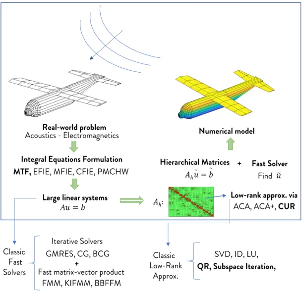
1.1 Integral approach for the solution of acoustics and electromagnetic problems (enclosed in the box) with classical approaches. In bold text we highlight the methods (formula-tions and low-rank approxima(formula-tions) that we shall use for the development of this thesis. 12

1.2 Wave scattering model problem . . . 13

1.3 Gap Idea of global MTF . . . 14

2.1 Geometrical configuration we consider in the analysis . . . 22

2.2 3D geometry for the numerical experiment . . . 25

2.3 Eigenvalues of the matrix M−1_ℎ ⋅ [MTFloc] ⋅ M−1_ℎ ⋅ [MTF−1loc] for σ = −1₂, with a zoom below around 1. . . 26

2.4 Convergence history of GMRES with a restart value of 40, case κ₀ = 1, κ₁= 6, κ₂ = 6. . 27

2.5 Convergence history of GMRES with a restart value of 40, case κ0 = 1, κ1= 5, κ2 = 10. . 27

3.1 Eigenvalue distribution with κ0 = κ1 = 2π/λ with λ = 0.5, μ0 = 1, μ1 = 2 (left) and μ₀= 2, μ₁= 1 (right). . . 36

3.2 Eigenvalue distribution with κ0 = κ1 = 2π/λ with λ = 1, μ0 = 1, μ1 = 2 (left) and μ0= 2, μ1= 1 (right). . . 36

3.3 Eigenvalue distribution with κ₀ = κ₁ = 2π/λ with λ = 10, μ₀ = 1, μ₁ = 2 (left) and μ0= 2, μ1= 1 (right). . . 36

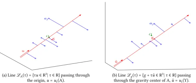
4.1 Error in maximum norm of rank 𝑘 = 10 approximations of a 100 × 100 random matrix A. 45 5.1 Best fitting lines (represented as arrows) of a matrix A = [𝑎1, ⋯ , 𝑎𝑛] ∈ ℝ3×𝑛. The small circles represent the columns 𝑎_𝑗’s, for 𝑗 = 1, ⋯ , 𝑛, and their projections over the lines are also showed. The gravity center 𝑔 and the matrix Y are defined in (5.2.4) and (5.2.5) respectively. . . 56

5.2 Convergence curves of the approximation error for the KAHAN matrix. . . 64

5.3 Convergence curves of the approximation error for the GKS matrix. . . 64

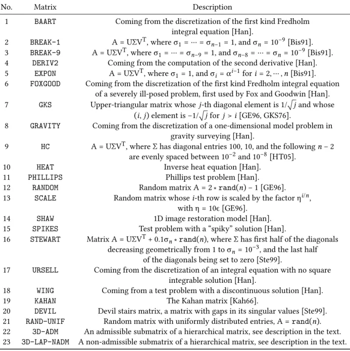
5.4 Convergence curves of the approximation error for the RAND-UNIF matrix. . . 65

5.5 Convergence curves of the approximation error for the SHAW matrix. The horizon-tal line is the threshold value, ϵ max(𝑚, 𝑛)‖A‖2, beyond which the singular values are considered as zero. . . 65

(9)

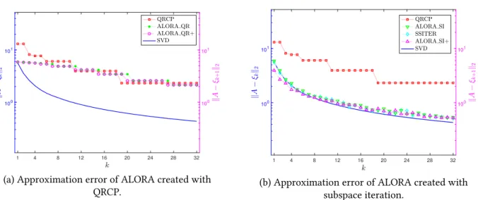
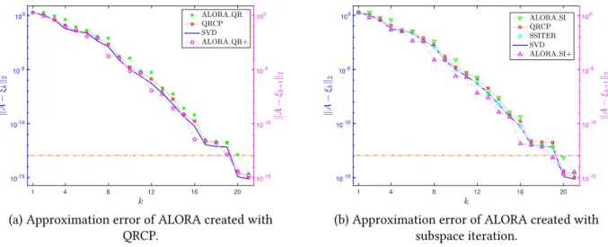
5.6 Convergence curves of the approximation error for the DERIV2 matrix. . . 65 5.7 Mean of the ratios of the errors of rank-𝑘 approximations created by ALORA_QR+ and

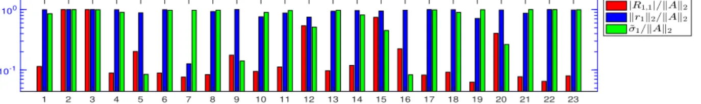
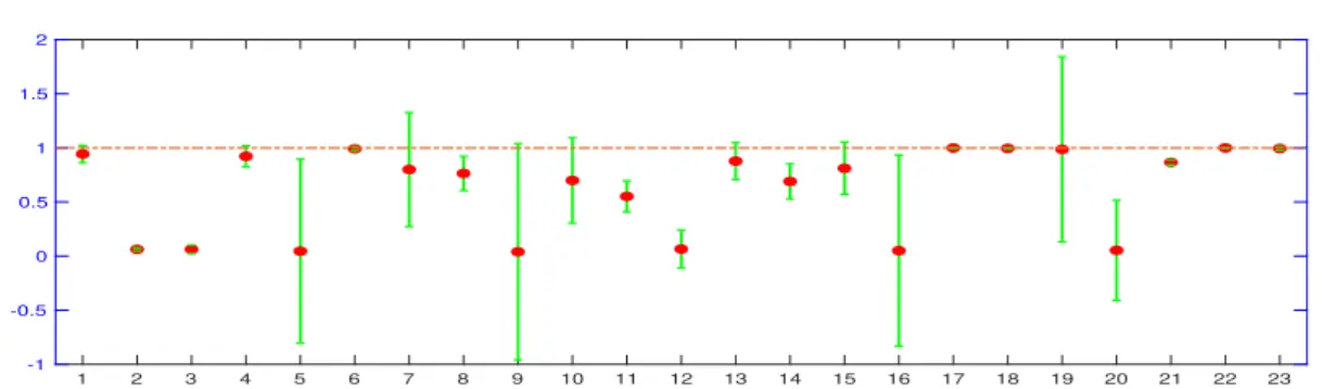
ALORA_SI+ to the optimal error. For each matrix, 𝑒_QRCP, 𝑒_{ALORA_QR+} and 𝑒_{ALORA_SI+} are, respectively, the mean of the vectors E_QRCP, E_{ALORA_QR+} and E_{ALORA_SI+}defined in (5.4.1), (5.4.2) and (5.4.3); and var_1, var_2 and var_3 are their variances. . . 66 5.8 Ratios of the approximated matrix norm, we compare |R(1, 1)|, ‖R(1, ∶)‖₂and ̃σ₁to ‖A‖₂. 67 5.9 Ratios of the error of rank-one approximation obtained by QRCP and ξ1from (5.3.15)

to the optimal error. . . 67 5.10 Correlation vector and coefficient for the 23 matrices from Table 5.1. . . 68 6.1 Interaction of distant subdomains on a sphere, and selection of representative target

points. . . 74 6.2 Surface from [Beb00], with admissible subdomains created with η = 0.15. . . 80 6.4 Error convergence of CUR approximation with geometric sampling. The values of δ(𝑘)

and det(M𝑘) allow to show the method that better approaches a maximal volume

sub-matrix. . . 81 6.5 Comparison of our linear cost method CUR_GS versus 𝒪(𝑚𝑛𝑘) cost methods QRCP and

ACAf. . . 81 6.6 Airplane surface with admissible subdomains created with η = 0.22. . . 82 6.7 Error convergence of CUR approximation with geometric sampling. The values of δ(𝑘)

ACAf. . . 83 6.9 Toroid surface with admissible subdomains created with η = 0.22. . . 83 6.10 Error convergence of CUR approximation with geometric sampling. The values of δ(𝑘)

ACAf. . . 84 6.12 Two admissible subdomains, created with η = 0.39. By computing their interaction via

the kernel function (6.4.3), they produce a matrix of type (6.4.4). . . 85 6.13 Error convergence of CUR approximation with geometric sampling. The values of δ(𝑘)

and det(M_𝑘) allow to show the method that better approaches a maximal volume sub-matrix. . . 85 6.14 Comparison of our linear cost method CUR_GS versus 𝒪(𝑚𝑛𝑘) cost methods QRCP and

ACAf. . . 86 6.15 3D cavity domain. . . 86 6.16 Comparison of the execution time and absolute approximation error between ACAp

and CUR_GCS . . . 87 A.1 Illustration of the tournament pivoting scheme on an 𝑚-by-10 matrix using 3 processors. The

red and blue nodes correspond to reduction trees inside each processor and inter-processors respectively. There are only two inter-processors messages, this number of messages (two) is independent of the number of columns and it is obviously optimal. . . 98 A.2 Error of approximation for PDGEKQP and CALRQR normalized with respect to the

truncated SVD error. . . 101 A.3 Scalability of CALRQR algorithm for large matrices, runtime measured assigning one

(10)

B.1 Ratio of classical bound B_Gfor QRCP (see Table 4.1) to the new bound B_Afrom Lemma 4.1. . . 106

(11)

List of Tables

4.1 Error bound for classical QR algorithms for a matrix A ∈ ℝ𝑚×𝑛, where 𝑘 is the truncation rank and ν is a constant. . . 46 5.1 Test matrices . . . 63 A.1 Performance models of parallel TSQR and ScaLAPACK’s parallel QR factorization

PDGE-QRF on a 𝑚 × 𝑛 matrix with P processors, along with lower bounds on the number of flops, words, and messages [DGHL08]. . . 97 A.2 Performance model of parallel all-reduction tournament pivoting to compute a full QR

factorization [DGGX15]. . . 98 A.3 Performance model of parallel tournament pivoting performed as a reduction operation

to select 𝑏 pivot columns. . . 99 A.4 Performance models of the two versions of CALRQR on a rectangular 𝑚 ×𝑛 matrix with

P processors, considering the rank of the matrix equal to b. “TP” stands for tournament pivoting. . . 101 A.5 Time, in seconds, to obtain a rank-256 QR truncated factorization of a set of large

(12)

CHAPTER

1

Introduction

1.1 Context of this work

Large scale modeling of real-world problems requires formulations and solvers that go hand in hand with the development of computational resources. Among these problems: acoustics, diffraction, fluid dynamics, electromagnetism, weather prediction, seismic modeling, etc. Boundary Integral Equations (BIE) naturally arise in such applications and have been extensively studied both at the theoretical and practical level. Abel (1826) was one of the first persons to formulate and solve an integral equation, which then lead to the search of integral forms of partial differential equations that govern natural phenomena. Nowadays, the challenge is to develop fast and accurate methods to solve these problems via formulations and algorithms that can be efficiently implemented in large scale computer clusters.

Since most integral equations can not be solved explicitly, BIE are, in general, solved numerically by using a standard approach known as Boundary Element Methods (BEM), which requires a so called integral formulation. Classical formulations for BEM are the electric field integral equation (EFIE), the magnetic field integral equation (MFIE), the combined field integral equation (CFIE), the PMCHW (Poggio, Miller, Chang, Harrington, and Wu) formulation, among others, refer to [JSC02] for a sur-vey. The first part of this thesis is devoted to a formulation for wave scattering problems in acoustics and electromagnetism. Albeit we focus on these particular fields, the presented theory is amenable to be extended to other fields. Wave scattering problems can be solved using the previously mentioned formulations, by reducing the continuous problem to a discrete one represented by a linear system, which is in general ill-conditioned and precondition techniques are necessary. Classical formulations such as the EFIE struggle to admit operator preconditioning when dealing with several scattering do-mains. For such case, Multi-trace formulations (MTF) [CH11, HJH12] are alternative approaches that

(13)

12 Chapter 1. Introduction are friendly to operator preconditioning and allow to have a linear system that essentially maintain a constant condition number while refining the problem mesh. The idea behind MTF is the use of domain decompositions techniques which make them amenable for large scale computational models.

Once we reduce a BIE problem to the solution of a linear system, the classical approach is to use iterative solvers such as the Generalized Minimal Residual Method (GMRES), Conjugate Gradient (CG), Bi-Conjugate Gradient (BCG), among others that can be found in [QSS06]. To accelerate such solvers we need a fast way to compute matrix-vector products which can be achieved by classical techniques like the Fast Multipole Method FMM [GR87, Kou95] or the more recent Kernel Independent and Black Box FMM (resp. KIFMM and BBFMM) [MR07, FD09]. Another strategy is to use hierarchical matri-ces [Beb08, Bör10, Hac15], which partition the matrix associated to the linear system in blocks that admit a low-rank approximation and those who do not. And then approximate low-rank blocks us-ing algorithms such as the Adaptive Cross Approximation (ACA) [Beb00] or its variants, e.g. ACA+ [Gra13].

Numerical model Integral Equations Formulation

Acoustics - Electromagnetics

MTF, EFIE, MFIE, CFIE, PMCHW

𝐴! = # Iterative Solvers FMM, KIFMM, BBFFM Hierarchical Matrices Classic Fast Solvers GMRES, CG, BCG

Large linear systems

Fast matrix-vector product

ACA, ACA+, CUR

$_ℎ&! = &#

$_ℎ_: Low-rank approx. via

+ + Fast Solver '! Find Real-world problem QR, Subspace Iteration, Classic Low-Rank Approx. SVD, ID, LU,

Figure 1.1: Integral approach for the solution of acoustics and electromagnetic problems (enclosed in the box) with classical approaches. In bold text we highlight the methods (formulations and low-rank

(14)

1.2. Multi-Trace formulations 13 In the second part of this thesis, we focus on techniques for low-rank matrix approximations. We start with a general framework for rectangular matrices, and then we analyze the particular case of matrices arising from BEM discretization. Classical low-rank approximations can be constructed via: the Singular Value Decomposition (SVD), QR or LU factorizations, Interpolative Decompositions (ID), Subspace Iteration, CUR decompositions, among others, refer to [KG17] for a survey. The scope of this thesis is summarized in Figure 1.1, which shows classical approaches to handle wave scattering problems (enclosed in a box), and highlights the methodologies that we shall use later on: integral MTF, hierarchical matrices, CUR decompositions, and general low-rank matrix approximations via QR factorizations and subspace iteration.

1.2 Multi-Trace formulations

As mentioned earlier, MTF are formulations that admit efficient operator preconditioning, for a survey on MTF refer to [CHJH13, CHJHP15]. These formulations come in two flavors based on different ideas. To give a simple and comprehensible introduction to MTF, let us consider a scattering problem in acoustics,

−ΔU − κ2_𝑖U = 0, (Helmholtz equation), or in electromagnetism,

−∇ × ∇ × E − κ2_𝑖E = 0, (Maxwell equation),

where we search solutions for U (resp. E). Let the problem be posed on a domain configuration as shown in Figure 1.2, where Ω𝑖is a Lipschitz domain and Γ𝑖𝑗refers to the intersection of the boundaries

of Ω𝑖and Ω𝑗, for 𝑖, 𝑗 = 0, 1, 2. The incident wave is given as U𝑖𝑛𝑐.

Ω

₀

U

inc

Ω

₁

Ω

₂

Γ

₀₁

Γ

₀₂

Γ

₁₂

Figure 1.2: Wave scattering model problem

The connection between these domains is stablished by transmission conditions. For acoustics, they consist in continuity of the solution and normal continuity of the gradient. For electromagnetism, tan-gential continuity of the electric and magnetic fields, c.f. chapter 3. By supplementing those conditions with a radiation condition at infinity, we can take for granted existence and uniqueness of solutions in the week sense, see e.g. [Pet89, CK13].

In general, integral formulations are oriented to find trace functions which are posed on the bound-aries Γ_𝑖𝑗, classical methods search for two trace functions known as Dirichlet and Neumann traces. Once these trace functions are obtained, using representation formulae, the solutions for U and E can be computed in the whole volume, see e.g. [Ste08].

(15)

14 Chapter 1. Introduction • Global-MTF: Introduced in [CH11], this formulation is based on a so called gap idea, consisting in tearing apart the scattering domains by a small separation δ > 0, see Figure 1.3. Then, proceed to write a classical formulation considering the new interfaces configuration and then make δ → 0.

Ω

₁

Ω

₂

$

Figure 1.3: Gap Idea of global MTF

For the global-MTF framework, we get four unknown trace functions on the middle interface Γ12,

two coming from the bottom and two coming from the top (instead of two as in the case of clas-sical formulations); hence, they are called multi-trace. Global-MTF is robust for both Helmholtz and Maxwell equations, and admits operator preconditioner (indeed, the global-MTF operator preconditions itself) allowing to deal with mesh refinement without making the condition num-ber of the discrete system to blow up. As a drawback, the global-MTF needs to perform the discretization of remote coupling operators which are non-local and when discretized yield to dense (compressible) matrices.

• Local-MTF: Introduced in [HJH12], it is based on local use of transmission conditions. For each domain Ω𝑖 two traces are obtained and the operator counts the contributions of the others

do-mains by using transmission operators which map traces on ∂Ω𝑗into traces on ∂Ω𝑖. These

oper-ators are purely local and, when discretized, yield to sparse matrices. Local-MTF admits a simple and robust preconditioning technique. As a drawback, its stability for Maxwell equation has not yet been proved. We devote the following two chapters to analyze this formulation and make contributions to its developments.

1.3 Matrix-compression and low-rank approximations

In the second part of this thesis, we are interested at first in low-rank approximations for a general rectangular matrix A ∈ ℂ𝑚×𝑛, and then we study the particular case where A arises from BEM dis-cretization. Let A𝑘 ∈ ℂ𝑚×𝑛be the rank-𝑘 matrix that minimizes the approximation error in the spectral

norm, A𝑘 can be obtained by the truncated SVD, [EG36, Mir60], and it holds that ‖A − A𝑘‖2 = σ𝑘+1,

where σ_𝑘+1is the 𝑘 + 1 singular value of A, and ‖ ⋅ ‖₂is the spectral matrix norm. Computing the trun-cated SVD is considered expensive in practice and fast techniques are commonly applied to search for good rank-𝑘 approximations.

Several low-rank approximations are linked to the Column Subset Selection Problem (CSSP), which consists in finding a set of 𝑘 columns of A given by an index vector J, such that the low-rank ma-trix ξ_𝑘, obtained by projecting the columns of A onto the space generated by the selected columns, approximates A with a minimal error. For a given choice of J, we have

(16)

1.4. Summary and Contributions 15 where 𝑓 is a small degree polynomial, C ∶= A(∶, J) ∈ ℂ𝑚×𝑘 is the matrix formed by the J selected columns, and C†is its classical Moore-Penrose pseudoinverse. Note that we can find the solution of the CSSP by analyzing (𝑛_𝑘) possible choices of J. However, it would cost 𝒪(𝑛𝑘) which is prohibitive in practice, and finding such solution is known to be NP-hard [ÇMI13]. Polynomial-cost methods for CSSP are extensively studied in the literature [DRVG06, DV06, BMD09] and there even exists algo-rithms that find suboptimal approximations in polynomial time [DR10].

Pivoted QR factorization techniques can be efficiently used to approximate the solution of the CSSP [CGMR05], providing efficient low-rank approximations that can even be proved to be suboptimal [GE96]. Low-rank QR based approximations will play a fundamental role in the development of the second part of this manuscript.

Another type of factorization, closely linked to the CSSP, is the CUR low-rank approximation [MD09, DR10, WZ13, VM17], which consists in finding J via an approximation of the CSSP, and then proceed to find a row index vector I of size 𝑘, selected such that the submatrix of C with row indices given by I, and denoted by C(I, ∶), is non-singular. Then A is approximated as

A ≈ C ⋅ U ⋅ R,

where C = A(∶, J), R ∶= A(I, ∶) ∈ ℂ𝑘×𝑛 and U ∶= C−1(I, ∶) ∈ ℂ𝑘×𝑘. When A is a matrix arising from BEM discretization, CUR methods are also known as skeleton approximations [GZT97, Beb00, GT01, GOS+08] and we devote an entire chapter to its numerical and algorithmic analysis.

To conclude, another kind of approximation that we shall use in this thesis, can be obtained via subspace iteration methods, c.f. §4.4, which consist in constructing a low-rank matrix by approximating the column space of Y ∶= (AAT)𝑞AΩ, where 𝑞 is a small integer parameter and Ω ∈ ℝ𝑛×𝑙 is a random matrix. We get A ≈ QB_𝑘, where Q ∈ ℂ𝑚×𝑘is the orthogonal basis of Y and B_𝑘 is the rank-𝑘 truncated SVD of QTA, see e.g. [Gu15, HMT11]. The bound on the error holds with high probability [HMT11]

𝔼‖A − QB_𝑘‖₂≤ (1 + (1 + 4 √ 2 min(𝑚, 𝑛) 𝑘 − 1 ) 1/(2𝑞+1) ) σ𝑘+1.

1.4 Summary and Contributions

This manuscript is structured in two parts that can be read independently. The first part deals with the solution of boundary integral equations arising from acoustics and electromagnetics problem, for which we use the multi-trace formulation. Then, in the second part of the thesis we propose methods of low-rank compression and approximation of general matrices for accelerating the solution of linear systems arising from BEM discretizations.

Part I

• In Chapter 2, we apply the local multi-trace formulation for acoustic scattering problems. We consider a model problem where all scattering domains are composed with an unique homoge-nous material and then we find a closed form for the inverse of the local-MTF operator corre-sponding to this configuration. We then use this inverse operator for preconditioning general composite scattering problems.

(17)

16 Chapter 1. Introduction • In Chapter 3, we analyze the stability of the local-MTF for the case of Maxwell equation, which was an open question in the literature of MTF. We prove the injectivity of the local Multi-Trace operator and then a generalized Gårding inequality for the local-MTF formulation on the unit sphere.

Part II

• In Chapter 4, we recall classical low-rank approximations for general matrices, focusing in par-ticular on QR and subspace iteration methods. For the former we provide a new bound on the error when the classical column pivoting technique is used; and furthermore, we prove a bound for the case when a general pivoting technique is used. For the latter, we prove exponential con-vergence on the approximation of singular vectors, which was an open question in the literature. • In Chapter 5, we introduce the concept of affine low-rank approximations providing an algorithm called ALORA that is intended to modify standard approximation algorithms. We then introduce a correlation coefficient to relate the spacial distribution of the columns of a matrix to its low-rank structure, which helps to understand for which matrices an affine low-low-rank approximation would be advantageous. Finally, we compare the performance of affine low rank-approximation with respect to standard QR and subspace iteration algorithms.

• In Chapter 6, we introduce the novel concept of geometric sampling to approximate matrices arising from BEM discretization, to which we refer as to BEM matrices. We provide a framework to constuct linear-time CUR approximations using information from the geometry where the problem is posed. We prove a general bound on the approximation error and provide a CUR algorithm that performs very well in practice using a criterion called gravity centers sampling. In Appendix A, we present an independent work, albeit related to the low-rank analysis performed in Chapter 4. It consists in a communication avoiding low-rank QR approximation algorithm developed during the first year of this thesis. Note that this work has not received any further development for two years. However, in a future work, this contribution could be optimized for particular applications to accelerate and increase the precision of matrix-compression and low-rank approximations.

Appendix B contains additional theoretical results and MATLAB codes corresponding to the work developed in the second part of this Thesis.

(18)

Part I

(19)

(20)

CHAPTER

2

Local Multi-Trace formulation

2.1 Preliminaries

The local multi-trace formulation (later abbreviated local-MTF) was introduced in [HJH12] as a means to solve acoustic wave scattering by heterogenous penetrable structures as those found in composite materials. The MTF considers as unknowns Dirichlet and Neumann traces on either side of the subdo-mains. These traces are then required to satisfy Calderón identities per subdomain and transmission conditions per interface. This last condition forces the appearance of restriction and extension-by-zero operators which entail Petrov-Galerkin variational forms: trial and test functions belong to different functional spaces, H±1/2(Γ) and ̃H∓1/2(Γ), respectively. Consequently, a mismatch between continuity and coercivity spaces takes place and, consequently, the Fredholm alternative argument cannot be used directly. Still, by using Lion’s lemma and by proving uniqueness of solutions, it is shown that the for-mulation is well-posed [HJH12, CHJH13].

For the discretization of local-MTF, one requires a slight increase in regularity and inverse discrete inequalities such as those presented in the original work for 2D (cf. [HJHM15] for 3D) to derive dis-crete stability estimates. However, numerically the method has been successfully shown to be easy to implement with standard codes, with clear parallelization and, though ill-conditioned, obvious pre-conditioners of algebraic or Calderón type. In recent years, a great deal of work has been devoted to either extend local-MTF [JHPT15], find alternative formulations [CHJH13, CHJHP15], find its con-nection domain decomposition methods [HJHLP14, DG16, JHPAT17] while with applications even in cellular simulation [HJHA16].

(21)

back-20 Chapter 2. Local Multi-Trace formulation ground for the theory presented in this and the following chapter. Then, we provide a closed form for the inverse of the local multi-trace operator of a model transmission problem, we posit that this inverse operator can be taken as a preconditioner for general local-MTF of composite scattering in acoustics. The chapter is structured as follows, in Section 2.2 we present technical concepts needed for our heavy analysis later on. Section 2.3 presents the local multi-trace operator and in Section 2.4 we derive its inverse for a model problem. Next, in Section 2.5 we numerically verify the theoretical analysis and show the efficiency of the obtained preconditioner. Finally, Section 2.6 concludes the chapter.

2.2 Functional and trace spaces

Let us consider a partition of the 𝑑 dimensional space ℝ𝑑 ∶= ⋃𝑛_𝑗=0Ω_𝑗 where each Ω_𝑗 is a connected Lipschitz domain. We refer Γ𝑗 ∶= ∂Ω𝑗 as the boundary of Ω𝑗.

Next, let L2(Ω) be the functional space given by the square integrable functions, and define the following functional spaces,

H1(Ω_𝑗) ∶= {𝑣 ∈ L2(Ω_𝑗_{) || ‖𝑣‖}2_H1_(Ω 𝑗)∶= ∫_Ω 𝑗 |𝑣|2+ |∇𝑣|2< +∞} , (2.2.1) H(div, Ω_𝑗) ∶= {𝑣 ∈ L2(Ω_𝑗_{) || ‖𝑣‖}2_H(Ω 𝑗)∶= ∫_Ω𝑗|𝑞| 2_{+ |div(𝑞)|}2_{< +∞} ,} _(2.2.2) H(curl, Ω_𝑗) ∶= {𝑣 ∈ L2(Ω_𝑗_{) || ‖𝑣‖}2_H(curl,Ω 𝑗)∶= ‖𝑣‖L2(Ω𝑗)+ ‖curl𝑣‖L2(Ω𝑗)< +∞} . (2.2.3)

If H(Ω_𝑗) is one of the functional spaces defined above, we define H_loc(Ω_𝑗) ∶= {𝑣 | φ𝑣 ∈ H(Ω_𝑗), ∀φ ∈ 𝒟 (ℝ𝑑)} , where 𝒟 (ℝ𝑑) is the space of functions of class 𝒞∞having compact support.

2.2.1 Trace spaces

The space of Dirichlet traces is given as

H1/2(Γ𝑗) ∶= {𝑣|Γ𝑗 || 𝑣 ∈ H1(Ω𝑗)} ,

equipped with the norm ‖𝑣‖_H1/2_(Γ

𝑗)∶= min {‖𝑢‖H1(Ω𝑗) || 𝑢 ∈ H 1_(Ω

𝑗), 𝑢|Γ𝑗 = 𝑣} ,

and the space of Neumann traces, H−1/2(Γ𝑗), is defined as the dual to H1/2(Γ𝑗) and is equipped with the

corresponding canonical dual norm

‖𝑝‖_H−1/2_(Γ𝑗)∶= sup 𝑣∈H1/2_(Γ𝑗)\{0} |⟨𝑝, 𝑣⟩| ..‖𝑣‖_H1/2_(Γ 𝑗) .

When dealing with Maxwell equation in the next chapter, letting Ω ⊂ ℝ3be a connected Lipschitz domain with Γ = ∂Ω, we shall refer to H−1/2(div, Γ) as the tangential traces of volume based vector fields belonging to H(curl, ℝ3),

(22)

2.3. Local Multi-Trace operator 21

H−1/2(div, Γ) ∶= {𝑢|_Γ× 𝑛_𝑗 || 𝑢 ∈ H(curl, ℝ3)} ,

note that this definition does not depend on the choice of the normal 𝑛𝑗. This space is put in duality

with itself by means of one of the bilinear forms 𝑢, 𝑣 ↦ ∫_Γ𝑛𝑗 ⋅ (𝑢 × 𝑣)𝑑σ. We also need to introduce

duality pairings for H−1/2(div, Γ)2= H−1/2(div, Γ) × H−1/2(div, Γ) that is defined by [(𝑢, 𝑝), (𝑣, 𝑞)]Γ𝑗 ∶= ∫

Γ𝑗

𝑛𝑗⋅ (𝑢 × 𝑞 + 𝑝 × 𝑣) 𝑑σ.

Multi-trace formulations will be written in a so-called multi-trace space and obtained as the carte-sian product of traces on the boundary of each subdomain. It takes the simple form

ℍ(Σ) ∶= H−1/2(div, Γ)2× H−1/2(div, Γ)2= H−1/2(div, Γ)4.

This space will be equipped with a bilinear pairing [[⋅, ⋅]] ∶ ℍ(Σ) × ℍ(Σ) → ℂ defined as follows. For any tuples 𝑢 = (𝑢0, 𝑢1), 𝑣 = (𝑣0, 𝑣1) ∈ ℍ(Σ) we set

[[𝑢, 𝑣]] ∶= [𝑢₀, 𝑣₀]_Γ0+ [𝑢₁, 𝑣₁]_Γ1.

Note the identity [[𝑢, 𝑣]] = −[[𝑣, 𝑢]] for any 𝑢, 𝑣 ∈ ℍ(Σ). Next we need to introduce three interior trace operators γ𝑗t, γ𝑗r ∶ H(curl, Ω𝑗) → H−1/2(div, Γ𝑗) and γ𝑗 ∶ H(curl, Ω𝑗) → H−1/2(div, Γ𝑗)2, those

traces are taken from the interior of Ω_𝑗and defined for all 𝑢 ∈ 𝒞∞(ℝ3)3by γ𝑗t(𝑢) ∶= 𝑢|Γ× 𝑛𝑗,

γ𝑗r(𝑢) ∶= curl(𝑢)|Γ× 𝑛𝑗,

γ𝑗(𝑢) ∶= (γ𝑗t(𝑢), γ𝑗r(𝑢)).

(2.2.4)

The trace operators γ𝑗t,𝑐(resp. γ𝑗r,𝑐, γ𝑗𝑐) shall refer to exactly the same operators as (2.2.4) but with

traces taken from the exterior (with the same direction of normal vector 𝑛𝑗 though). Then we shall

define jump and averages traces as

{γ𝑗⋆}(𝑢) ∶= (γ𝑗⋆(𝑢) + γ𝑗⋆,𝑐(𝑢))/2,

[γ𝑗⋆](𝑢) ∶= γ𝑗⋆(𝑢) − γ𝑗⋆,𝑐(𝑢) for ⋆ = t, r.

(2.2.5) We define {γ𝑗} and [γ𝑗] accordingly.

2.3 Local Multi-Trace operator

We start by introducing the local multi-trace formulation for a model problem. Consider a partition of the space ℝ𝑑 = Ω0∪ Ω1∪ Ω2as shown in Figure 2.1.

(23)

22 Chapter 2. Local Multi-Trace formulation

Figure 2.1: Geometrical configuration we consider in the analysis

We assume that Ω𝑗, 𝑗 = 0, 1, 2 are Lipschitz domains such that Ω𝑗∩ Ω𝑘 = ∅ for 𝑗 ≠ 𝑘. Denoting by

Γ_𝑗 ∶= ∂Ω_𝑗, we assume in addition that Γ₁∩ Γ₂ = ∅ and Γ₀ = Γ₁∪ Γ₂. Let 𝑛_𝑗 be the unit outer normal for Ω𝑗on its boundary Γ𝑗. For a sufficiently regular function 𝑣 we denote by 𝑣|+Γ𝑗the trace of 𝑣 and by

∂𝑛𝑗𝑣| +

Γ𝑗 the trace of 𝑛𝑗⋅ ∇𝑣 on Γ𝑗taken from inside of Ω𝑗. Similarly we define 𝑣| −

Γ𝑗 and ∂𝑛𝑗𝑣| −

Γ𝑗 but with

traces from outside of Ω𝑗.

The elliptic transmission problem for which we want to study the local multi-trace formulation and its inverse is: find 𝑢 ∈ H1(ℝ𝑑) such that

−Δ𝑢 + κ2_𝑗𝑢 = 0 in Ω𝑗, 𝑗 = 0, 1, 2,

[𝑢]Γ1 = 𝑔1, [𝑢]Γ2= 𝑔2,

[∂𝑛𝑢]Γ1= ℎ1, [∂𝑛𝑢]Γ2= ℎ2,

(2.3.1) where κ𝑗 > 0 for 𝑗 = 0, 1, 2, 𝑔𝑗 ∈ H+1/2(Γ𝑗) and ℎ𝑗 ∈ H−1/2(Γ𝑗) are given data of the transmission

problem, and we used the classical jump notation for the Dirichlet and Neumann traces of the solution across the interfaces Γ𝑗, 𝑗 = 1, 2, i.e. [𝑢]Γ𝑗 ∶= 𝑢|

+ Γ𝑗− 𝑢| − Γ𝑗and [∂𝑛𝑢]Γ𝑗 ∶= ∂𝑛𝑗𝑢| + Γ𝑗− ∂𝑛𝑗𝑢| − Γ𝑗.

Following [HJHLP14], this problem can be rewritten as a boundary integral local multi-trace for-mulation, using the Calderón projector: let ℍ(Γ𝑗) ∶= H1/2(Γ𝑗) × H−1/2(Γ𝑗); then for (𝑔, ℎ) ∈ ℍ(Γ𝑗), the

Calderón projector ℙ𝑗∶ ℍ(Γ𝑗) → ℍ(Γ𝑗) interior to Ω𝑗associated to the operator −Δ + κ2𝑗 is defined by

ℙ_𝑗(𝑔, ℎ) ∶= (𝑣|+_Γ_𝑗, ∂_𝑛𝑗𝑣|+_Γ_𝑗) where 𝑣 satisfies −Δ𝑣 + κ2_𝑗𝑣 = 0 in Ω𝑗 and in ℝ𝑑 ⧵ Ω𝑗,

[𝑣]Γ𝑗 = 𝑔 and [∂𝑛𝑣]Γ𝑗 = ℎ, and

lim sup_|𝑥|→∞|𝑣(𝑥)| < +∞,

and ℙ_𝑗is known to be a continuous map, see [SS11]. The decomposition Γ₀= Γ₁∪ Γ₂induces a natural decomposition of ℙ0in the following manner: for any U ∈ ℍ(Γ0) set ρ𝑗(U) ∶= U|Γ𝑗 ∈ ℍ(Γ𝑗), 𝑗 = 1, 2. In

addition, for any V ∈ ℍ(Γ𝑗), 𝑗 = 1, 2, define ρ∗𝑗(V) ∈ ℍ(Γ0) by ρ∗𝑗(V) = V on Γ𝑗and ρ∗𝑗(V) = 0 on Γ0⧵ Γ𝑗.

Then the projector ℙ₀can be decomposed as ℙ0= [ _R ̃ℙ1 R1,2/2

2,1/2 ̃ℙ2 ] , where {

̃ℙ_𝑗 ∶= ρ𝑗⋅ ℙ0⋅ ρ∗𝑗,

R𝑗,𝑘/2 ∶= ρ𝑗⋅ ℙ0⋅ ρ∗𝑘.

The operators ̃ℙ𝑗 ∶ ℍ(Γ𝑗) → ℍ(Γ𝑗) and R𝑗,𝑘 ∶ ℍ(Γ𝑘) → ℍ(Γ𝑗) are continuous. Following this

(24)

2.3. Local Multi-Trace operator 23 X(𝑣, 𝑞) ∶= (𝑣, −𝑞), and a relaxation parameter σ ∈ ℂ\{0}. The local multi-trace formulation of problem (2.3.1) is then: find (U1, U(0)1 , U(0)2 , U2) ∈ ℍ(Γ1)2× ℍ(Γ2)2such that

⎡ ⎢ ⎢ ⎢ ⎣ (1 + σ)Id − ℙ₁ −σX 0 0 −σX (1 + σ)Id − ̃ℙ1 −R1,2/2 0 0 −R2,1/2 (1 + σ)Id − ̃ℙ2 −σX 0 0 −σX (1 + σ)Id − ℙ2 ⎤ ⎥ ⎥ ⎥ ⎦ ⋅ ⎡ ⎢ ⎢ ⎢ ⎣ U1 U(0)₁ U(0)₂ U2 ⎤ ⎥ ⎥ ⎥ ⎦ = F, (2.3.2)

where F ∈ ℍ(Γ1)2× ℍ(Γ2)2is some right-hand side depending on 𝑔𝑗, ℎ𝑗, σ whose precise expression is

not important for our present study, where we want to obtain an explicit expression for the operator in (2.3.2) and its inverse for the special case

κ₀ = κ₁= κ₂. (2.3.3)

To simplify the calculations when working with the entries of the operator in (2.3.2), we set A_𝑗 ∶= −Id + 2ℙ_𝑗 and ̃A_𝑗 ∶= −Id + 2 ̃ℙ_𝑗. The following remarkable identities were established in [CDG18, §4.4] for the special case (2.3.3): ℙ2_𝑗 = ℙ_𝑗, ̃ℙ2_𝑗 = ̃ℙ_𝑗, ̃ℙ₁R_1,2 = ̃ℙ₂R_2,1 = 0, Xℙ_𝑗X = Id − ̃ℙ_𝑗, and finally R1,2R2,1= R2,1R1,2 = 0. These five properties can be reformulated in terms of the operators A𝑗, namely

𝑖) A2_𝑗 = ̃A2_𝑗 = Id,

𝑖𝑖) ̃A1R1,2= −R1,2and ̃A2R2,1= −R2,1,

𝑖𝑖𝑖) X ⋅ A𝑗⋅ X = − ̃A𝑗,

𝑖𝑣) R1,2R2,1= R2,1R1,2= 0,

𝑣) R1,2 ̃A2= R1,2and R2,1 ̃A1= R2,1.

(2.3.4)

Let us introduce auxiliary operators 𝔸, Π ∶ ℍ(Γ₁)2× ℍ(Γ₂)2defined by

𝔸 ∶= ⎡ ⎢ ⎢ ⎢ ⎣ A₁ 0 0 0 0 ̃A1 R1,2 0 0 R2,1 ̃A2 0 0 0 0 A2 ⎤ ⎥ ⎥ ⎥ ⎦ , Π ∶= ⎡ ⎢ ⎢ ⎢ ⎣ 0 X 0 0 X 0 0 0 0 0 0 X 0 0 X 0 ⎤ ⎥ ⎥ ⎥ ⎦ . (2.3.5)

According to property i) in (2.3.4), we have (Id + 𝔸)2/4 = (Id + 𝔸)/2, which implies the well known Calderón identity from the boundary integral equation literature, i.e.

𝔸2 = Id, (2.3.6)

see for example [Néd01, §4.4]. The local multi-trace operator on the left-hand side of Equation (2.3.2) can then be rewritten as

MTF_loc∶= −1

2𝔸 − σΠ + (σ + 1

2)Id. (2.3.7)

In (2.3.2), the terms associated with the relaxation parameter σ, namely Id − Π, enforce the trans-mission conditions of problem (2.3.1). For σ = 0, we have MTF_loc= 1₂(Id − 𝔸), which is a projector, and MTF_locis thus not invertible. For σ ≠ 0 however, MTF_loc was proved to be invertible in [Cla16, Cor. 6.3]. The goal of this chapter is to derive an explicit formula for the inverse of MTFloc, and we will thus

(25)

24 Chapter 2. Local Multi-Trace formulation

2.4 Inverse of the Local Multi-Trace Operator

We now derive a closed form inverse of the local multi-trace operator in (2.3.7) for the special case (2.3.3). Using that Π2 = Id and (2.3.6), we obtain

[ −𝔸/2 − σΠ + (σ + 1/2)Id ] [ −𝔸/2 − σΠ − (σ + 1/2)Id ] = (𝔸/2 + σΠ)2− (σ + 1/2)2Id

= (σ2+ 1/4 − σ2− σ − 1/4)Id + σ(𝔸Π + Π𝔸)/2 = −σId + σ(𝔸Π + Π𝔸)/2.

(2.4.1) Inspired by the calculations in [CDG18, §4.4] as well as [Cla16, Prop. 6.1], we examine more closely 𝔸Π + Π𝔸. We start by comparing 𝔸Π and Π𝔸:

𝔸Π = ⎡ ⎢ ⎢ ⎢ ⎣ 0 A1X 0 0 ̃A₁X 0 0 R1,2X R_2,1X 0 0 ̃A₂X 0 0 A2X 0 ⎤ ⎥ ⎥ ⎥ ⎦ , Π𝔸 = ⎡ ⎢ ⎢ ⎢ ⎣ 0 X ̃A₁ XR_1,2 0 XA1 0 0 0 0 0 0 XA2 0 XR2,1 X ̃A2 0 ⎤ ⎥ ⎥ ⎥ ⎦ . (2.4.2)

According to Property iii) in (2.3.4), we have X ̃A_𝑗+ A_𝑗X = 0 and XA_𝑗+ ̃A_𝑗X = 0, and thus from (2.4.2) we obtain Π𝔸 + 𝔸Π = ⎡ ⎢ ⎢ ⎢ ⎣ 0 0 XR1,2 0 0 0 0 R1,2X R_2,1X 0 0 0 0 XR2,1 0 0 ⎤ ⎥ ⎥ ⎥ ⎦ .

Computing the square of this operator, and taking into account Property iv) from (2.3.4), we obtain (Π𝔸 + 𝔸Π)2 = ⎡ ⎢ ⎢ ⎢ ⎣ XR_1,2R_2,1X 0 0 0 0 R1,2R2,1 0 0 0 0 R2,1R1,2 0 0 0 0 XR_2,1R_1,2X ⎤ ⎥ ⎥ ⎥ ⎦ = 0.

From this we conclude that (−Id + (𝔸Π + Π𝔸)/2)−1 = −Id − (𝔸Π + Π𝔸)/2. Coming back to (2.4.1), we obtain a first expression for the inverse of the local multi-trace operator, namely

[ −𝔸/2 − σΠ + (σ + 1/2)Id ]−1

= σ−1[ 𝔸/2 + σΠ + (σ + 1/2)Id ] [Id + (𝔸Π + Π𝔸)/2]

= σ−1[1₂(1 + σ)𝔸 + (σ + 1/4)Π + (σ + 1/2)(Id + (𝔸Π + Π𝔸)/2)] + σ−1[σ₂Π𝔸Π +1₄𝔸Π𝔸].

(2.4.3)

The only terms that are not explicitly known yet in (2.4.3) are the last two, Π𝔸Π and 𝔸Π𝔸. Combining (2.4.2) with the definitions given in (2.3.5), direct calculation yields

Π𝔸Π = ⎡ ⎢ ⎢ ⎢ ⎣ −A1 0 0 XR1,2X 0 − ̃A1 0 0 0 0 − ̃A₂ 0 XR2,1X 0 0 −A2 ⎤ ⎥ ⎥ ⎥ ⎦ , and similarly, we also obtain

𝔸Π𝔸 = ⎡ ⎢ ⎢ ⎢ ⎣ 0 −X XR_1,2 0 −X 0 0 −R1,2X −R2,1X 0 0 −X 0 XR_2,1 −X 0 ⎤ ⎥ ⎥ ⎥ ⎦ .

(26)

2.5. Numerical Experiments 25 We have now derived an explicit expression for each term in (2.4.3), which leads to a close form matrix expression for the inverse of the local multi-trace operator, namely

MTF−1_loc= (1 + 1 2σ)Id + 1 σ ⎡ ⎢ ⎢ ⎢ ⎢ ⎢ ⎣ 1 2A1 σX σ+1 2 XR1,2 σ 2XR1,2X σX 1₂ ̃A1 σ+1₂ R1,2 σ₂R1,2X σ 2R2,1X σ+1 2 R2,1 1 2 ̃A2 σX σ 2XR2,1X σ+1 2 XR2,1 σX 1 2A2 ⎤ ⎥ ⎥ ⎥ ⎥ ⎥ ⎦ . (2.4.4)

The expression MTFloc⋅ MTF−1loc = Id should not be mistaken for the Calderón identity (2.3.6). The

primary difference is that (2.4.4) involves coupling terms between Ω1 and Ω2, whereas in (2.3.6), all

three subdomains are decoupled.

2.5 Numerical Experiments

2.5.1 Verifying the inversion formula

We now illustrate the closed form inversion formula (2.4.4) for the local multi-trace formulation by a numerical experiment. We consider a three dimensional version of the geometrical setting described at the beginning in Figure 2.1. Here Ω₁ ∶= B(0, 0.5) is the open ball centered at 0 with radius 0.5, Ω2∶= ℝ3\[−1, +1]3, and Ω0∶= ℝ3⧵ Ω1∪ Ω2, see Figure 2.2.

Figure 2.2: 3D geometry for the numerical experiment

For our numerical results, we discretize both MTFlocgiven by (2.3.7) leading to a matrix we denote

by [MTF_loc], and MTF−1_locgiven by (2.4.4) leading to a matrix denoted by [MTF−1_loc]. Our discretization using the code bemtool1is based on a Galerkin method where both Dirichlet and Neumann traces are approximated by means of continuous piece-wise linear functions on the same mesh. We use a trian-gulation with a mesh width ℎ = 0.35, and generated the mesh using Gmsh, see [GR09].

Let Mℎbe the mass matrix associated with the duality pairing used to write (2.3.2) in variational

form. We represent the spectrum of the matrix M−1_ℎ ⋅ [MTFloc] ⋅ M−1_ℎ ⋅ [MTF−1loc] in Figure 2.3. We see that 1_{available on https://github.com/xclaeys/bemtool under Lesser Gnu Public License.}

(27)

26 Chapter 2. Local Multi-Trace formulation -1.5 -1 -0.5 0 0.5 1 1.5 -1.5 -1 -0.5 0 0.5 1 1.5 -0.02 -0.015 -0.01 -0.005 0 0.005 0.01 0.015 0.02 0.98 1 1.02 1.04 1.06 1.08

Figure 2.3: Eigenvalues of the matrix M−1_ℎ ⋅ [MTF_loc] ⋅ M−1_ℎ ⋅ [MTF−1_loc] for σ = −1₂, with a zoom below around 1.

the eigenvalues are clustered around 1, which agrees well with our analysis at the continuous level.

2.5.2 Preconditioner efficiency

Let us consider the operator P ∶= MTF−1_loc, obtained by choosing σ = −1₂ and considering a constant wave number κ₀ = 1 for all operators in equation (2.4.4). In this section, we evaluate the performance of P for preconditioning the local-MTF operator corresponding to a composite scattering problem in heterogenous media. We use the same domain as in section 2.5.1 and consider the problem of finding the solution 𝑢 of the following operator equation,

M(κ0, κ1, κ2)𝑢 = 𝑏, (2.5.1)

where 𝑏 is a constant 1-valued function and M(κ₀, κ₁, κ₂) denotes the local-MTF operator considering the wave numbers different in each domain and given as κ0 = 1, κ1 and κ2respectively in Ω0, Ω1 and

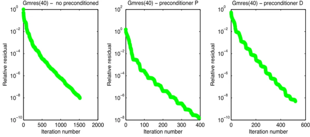
Ω₂. Next, we use P for preconditioning (2.5.1). Then, we discretize the problem to obtain a linear system which we solve using GMRES with a restart value of 40 and a tolerance of 10−8.

In figures 2.4 and 2.5 we present representative numerical tests which show that P is an efficient operator preconditioner for the local-MTF operator, and its effect is more notorious when the wave numbers are close to each other, which is in agreement with the theory. We compare our precondi-tioning technique against the classical block diagonal precondiprecondi-tioning operator D, which was used in the paper introducing local-MTF [HJH12, Sec. 5.3], given as

(28)

2.6. Conclusions of the chapter 27 D ∶= ⎡ ⎢ ⎢ ⎢ ⎣ A₁ 0 0 0 0 ̃A1 0 0 0 0 ̃A2 0 0 0 0 A2 ⎤ ⎥ ⎥ ⎥ ⎦ . 0 500 1000 10−10 10−8 10−6 10−4 10−2 100 Gmres(40) − no preconditioned Iteration number Relative residual 0 20 40 60 10−8 10−6 10−4 10−2 100 102 Gmres(40) − preconditioner P Iteration number Relative residual 0 100 200 300 10−8 10−6 10−4 10−2 100 102 Gmres(40) − preconditioner P_k Iteration number Relative residual 0 200 400 600 10−10 10−8 10−6 10−4 10−2 100 Gmres(40) − preconditioner D_k Iteration number Relative residual 0 500 1000 10−10 10−8 10−6 10−4 10−2 100 Gmres(40) − no preconditioned Iteration number Relative residual 0 20 40 60 10−8 10−6 10−4 10−2 100 102 Gmres(40) − preconditioner P Iteration number Relative residual 0 100 200 300 10−8 10−6 10−4 10−2 100 102 Gmres(40) − preconditioner P_k Iteration number Relative residual 0 200 400 600 10−10 10−8 10−6 10−4 10−2 100 Gmres(40) − preconditioner D_k Iteration number Relative residual 0 500 1000 10−10 10−8 10−6 10−4 10−2 100 Gmres(40) − no preconditioned Iteration number Relative residual 0 20 40 60 10−8 10−6 10−4 10−2 100 102 Gmres(40) − preconditioner P Iteration number Relative residual 0 100 200 300 10−8 10−6 10−4 10−2 100 102 Gmres(40) − preconditioner P_k Iteration number Relative residual 0 200 400 600 10−10 10−8 10−6 10−4 10−2 100 Gmres(40) − preconditioner D_k Iteration number Relative residual

Figure 2.4: Convergence history of GMRES with a restart value of 40, case κ₀ = 1, κ₁= 6, κ₂ = 6.

0 500 1000 1500 2000 10−10 10−8 10−6 10−4 10−2 100 Gmres(40) − no preconditioned Iteration number Relative residual 0 100 200 300 400 10−8 10−6 10−4 10−2 100 102 Gmres(40) − preconditioner P Iteration number Relative residual 0 500 1000 1500 2000 10−10 10−8 10−6 10−4 10−2 100 Gmres(40) − preconditioner P_k Iteration number Relative residual 0 200 400 600 10−10 10−8 10−6 10−4 10−2 100 Gmres(40) − preconditioner D_k Iteration number Relative residual 0 500 1000 1500 2000 10−10 10−8 10−6 10−4 10−2 100 Gmres(40) − no preconditioned Iteration number Relative residual 0 100 200 300 400 10−8 10−6 10−4 10−2 100 102 Gmres(40) − preconditioner P Iteration number Relative residual 0 500 1000 1500 2000 10−10 10−8 10−6 10−4 10−2 100 Gmres(40) − preconditioner P_k Iteration number Relative residual 0 200 400 600 10−10 10−8 10−6 10−4 10−2 100 Gmres(40) − preconditioner D_k Iteration number Relative residual 0 500 1000 1500 2000 10−10 10−8 10−6 10−4 10−2 100 Gmres(40) − no preconditioned Iteration number Relative residual 0 100 200 300 400 10−8 10−6 10−4 10−2 100 102 Gmres(40) − preconditioner P Iteration number Relative residual 0 500 1000 1500 2000 10−10 10−8 10−6 10−4 10−2 100 Gmres(40) − preconditioner P_k Iteration number Relative residual 0 200 400 600 10−10 10−8 10−6 10−4 10−2 100 Gmres(40) − preconditioner D_k Iteration number Relative residual

Figure 2.5: Convergence history of GMRES with a restart value of 40, case κ₀= 1, κ₁= 5, κ₂= 10.

2.6 Conclusions of the chapter

We have shown that it is possible for the local multi-trace operator of a model transmission problem to obtain a closed form for the inverse. This would therefore be an ideal preconditioner for local multi-trace formulations. The closed form inverse seems to be inherent to the formulation, and not dependent on the specific form of the partial differential equation. An open question that stems from this chapter is if such closed form inverses can also be obtained for more general situations, where the coefficients are only constant in each subdomain, and in the presence of more subdomains.

(29)

CHAPTER

3

Stability of Local-MTF for Maxwell equation

3.1 Preliminaries

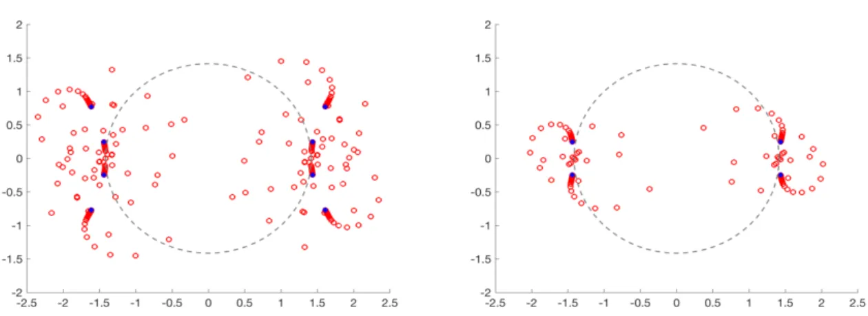
In this chapter, we study the local-MTF for an electromagnetic problem posed in a geometric configu-ration consisting in two subdomains and one interface, where one subdomain is the open unit ball, and the interface is the unit sphere. Our goal is to investigate the stability of the local-MTF for Maxwell in this precise setting. For this, we first prove that the local multi-trace operator is injective and then we write the local-MTF formulation in full detail by means of separation of variables based on vector spherical harmonics. We derive an explicit formula for the corresponding boundary integral operator, relying only on special functions (spherical Bessel and Hankel functions). We end this chapter plotting the first eigenvalues of the operator and commenting on the stability.

This chapter is structured as follows, in Section 3.2 we state the problem and background concepts needed for the analysis later on. Section 3.3 presents the local multi-trace operator for this framework and then a prove that such operator is injective. In Sections 3.4 and 3.5 we use a separation of variables technique based on vector spherical harmonics to derive explicit formulae for the local-MTF operator and the accumulation points of its spectrum. In Section 3.6, we numerically verify the theoretical analysis and in Section 3.7 we discuss on the stability of local-MTF for Maxwell equations. Finally, Section 3.8 concludes the chapter.

(30)

3.2. Problem setting 29

3.2 Problem setting

We consider a partition of free space as ℝ3 = Ω0∪ Ω1 in two smooth open subdomains, Ω0 and Ω1,

such that Ω0 = ℝ3 ⧵ Ω1. We denote Γ = ∂Ω0 = ∂Ω1 and let 𝑛𝑗 refer to the unit normal vector to Γ𝑗

directed toward the exterior of Ω_𝑗, so that we have 𝑛₀ = −𝑛₁. Let ϵ_𝑗 > 0 (resp. μ_𝑗 > 0) refer to the electric permittivity (resp. magnetic permeability) in domain Ω𝑗. We are interested in the scattering of

an incident electromagnetic wave (Einc, Hinc) propagating in harmonic regime at pulsation ω > 0. The

equations under consideration then write

⎧ ⎨ ⎩ curl(E) − 𝚤ωμ𝑗H = 0 curl(H) + 𝚤ωϵ𝑗E = 0 √μ0(H − Hinc) × ̂𝑥 − √ϵ0(E − Einc) = 𝒪|𝑥|→∞(|𝑥|−2) (3.2.1) {𝑛0× E|Γ0+ 𝑛1× E|Γ1 = 0 𝑛0× H|Γ0+ 𝑛1× H|Γ1= 0 (3.2.2) where we assume that curl(E_inc) − 𝚤ωμ₀H_inc= 0 in ℝ3and curl(H_inc) + 𝚤ωϵ₀E_inc= 0 in ℝ3; the incident field may be, for example, a plane wave. In addition, in the problem above ̂𝑥 ∶= 𝑥/|𝑥|. In Equation (3.2.2) the notation ”E|Γ𝑗” (resp. ”H|Γ𝑗”) should be understood as the trace taken at Γ from the interior of Ω𝑗.

Next, let us point out that (3.2.1)-(3.2.2) can be reformulated as a second order transmission boundary value problem, which is the basis of Stratton-Chu potential theory, given as,

{curl

2_{(E) − κ}2

𝑗E = 0 in Ω𝑗

curl(E − E_inc) × ̂𝑥 − 𝚤κ₀(E − E_inc) = 𝒪_|𝑥|→∞(|𝑥|−2) (3.2.3)

{𝑛0× E|Γ0+ 𝑛1× E|Γ1= 0

μ−1₀ 𝑛0× curl(E)|Γ0+ μ −1

1 𝑛1× curl(E)|Γ1= 0

(3.2.4) In the equations above we adopted the following notations for effective wave number in each subdo-main

κ𝑗 ∶= ω√μ𝑗ϵ𝑗, 𝑗 = 0, 1. (3.2.5)

We wish to study the solution of this problem by means of a boundary integral formulation. There are several possible such formulations. We focus here on the local Multi-Trace formulation (local-MTF). Since a complete stability analysis of local-MTF is not presently available, we will concentrate on the following special case.

Assumption: Ω1is the unit ball and Γ is the unit sphere.

This will allow explicit calculus by means of separation of variables which will help to investigate and clarify the structure of operators associated to the local-MTF.

3.3 Local multi-trace operator for Maxwell equation

For the mathematical analysis, we heavily rely on potential theory for electromagnetics, i.e Statton-Chu theory. On the sequel, 𝒢κ(𝑥) ∶= exp(𝚤κ|𝑥|)/(4π|𝑥|) will refer to the outgoing Green kernel of the

(31)

30 Chapter 3. Stability of Local-MTF for Maxwell equation Helmholtz equation with wave number κ > 0. Next we define the integral operators: for 𝑢 = (𝑢, 𝑝) ∈ H−1/2(div, Γ)2, we set G_κ(𝑢)(𝑥) ∶= DL_κ(𝑢)(𝑥) + SL_κ(𝑝)(𝑥), where SLκ(𝑝)(𝑥) ∶= κ−2_∫ Γ∇𝒢κ(𝑥 − 𝑦)divΓ𝑝(𝑦)𝑑σ(𝑦) + ∫Γ𝒢κ(𝑥 − 𝑦)𝑝(𝑦)𝑑σ(𝑦), where DLκ(𝑢)(𝑥) ∶= curl ∫ Γ𝒢κ(𝑥 − 𝑦)𝑢(𝑦)𝑑σ(𝑦).

The potential operator G_κcontinuously maps H−1/2(div, Γ)2into H_loc(curl, Ω₀) and it also satisfies (curl2 − κ2₀)Gκ(𝑢) = 0 in Ω0 as well as a Silver-Müller radiation condition at infinity, regardless of

𝑢 ∈ H−1/2(div, Γ)2. A similar result also holds in Ω1. The potential operator plays a central role in

the derivation of boundary integral equations as it can be used to represent solution to homogeneous Maxwell equations according to the Stratton-Chu representation theorem given as follows, c.f. [BH03, Thm. 6].

Theorem 3.1. Let U ∈ Hloc(curl, Ω𝑗) satisfy curl2(U) − κ2𝑗U = 0 in Ω𝑗. For 𝑗 = 0 assume in addition

that curl(U) × ̂𝑥 − 𝚤κ0U = 𝒪(|𝑥|−2) for |𝑥| → ∞. Then,

Gκ(γ𝑗(U))(𝑥) = 1Ω𝑗(𝑥)U(𝑥),

for all 𝑥 ∈ ℝ3.

On the other hand, the jumps of trace, c.f. (2.2.5), of the potential operator follow a simple and explicit expression given by the following proposition which can be found in [BH03, Thm. 7].

Proposition 3.1. For any 𝑢 ∈ H−1/2(div, Γ)2we have [γ𝑗] ⋅ Gκ(𝑢) = 𝑢.

In the forthcoming analysis, we shall make intensive use of the operator A𝑗_κ ∶= 2{γ𝑗} ⋅ G_κ. From the classical theory of potentials, it is clear that {γ𝑗t} ⋅ DLκ = {γ𝑗r} ⋅ SLκ, see e.g. [Ste08, SS11]. On the

other hand, using the vector Helmholtz equation satisfied by ∫_Γ𝒢_κ(𝑥 − 𝑦)𝑢(𝑦)𝑑σ(𝑦), we get also that {γ𝑗r} ⋅ DLκ= κ2{γ𝑗t} ⋅ SLκ. As a consequence the operator A𝑗κcan be represented in matrix form as

A𝑗_κ∶= [ κK𝑗κ κ−1V𝑗κ

κV𝑗_κ κ−1K𝑗_κ ] where {

V𝑗_κ∶= (2/κ){γ𝑗r} ⋅ DLκ,

K𝑗_κ∶= 2{γ𝑗t} ⋅ DLκ. (3.3.1)

Observe that, for a given κ we have A0_κ= −A1_κdue to the change in the orientation of the normals 𝑛0 = −𝑛1. The following proposition states that the operators in (3.3.1) can be used to characterize

solutions of Maxwell equations in a given subdomain.

Proposition 3.2. The operator γ𝑗G_κ= (Id+A𝑗_κ)/2 is a continuous projector as a mapping from H−1/2(div, Γ)2

into H−1/2(div, Γ)2. Its range is the space of traces γ𝑗(U), where U ∈ H_loc(curl, Ω_𝑗) satisfies

curl2(U) − κ2U = 0 in Ω_𝑗,

as well as

curl(U) × ̂𝑥 − 𝚤κ₀U = 𝒪(|𝑥|−2), for |𝑥| → ∞ if𝑗 = 0.

An easy consequence of the above proposition is that (A𝑗_κ)2 = Id which is known as Calderón’s identity. The incident field is solution to Maxwell equations with wave number κ0 on ℝ3 including

inside Ω1, so that we get (A1κ0− Id)γ 1_(E

(32)

3.3. Local multi-trace operator for Maxwell equation 31 hand A1_κ₀= −A0_κ₀and γ0(E_inc) = −γ1(E_inc) (continuity across interfaces), we conclude that A0_κ₀γ1(E_inc) = −γ1(Einc). Using Proposition 3.2, we also observe that equations (3.2.3) can be reformulated as

(A1_κ₁− Id)γ1(E) = 0, and,

(A0_κ₀− Id)(γ0(E) − γ0(Einc)) = 0,

where the later is equivalent to (A0_κ₀− Id)γ0(E) = −2γ0(E_inc).

Next, we need to reformulate the transmission conditions (3.2.4). Since these conditions are weighted with the permeability coefficients μ_𝑗, we need to introduce scaling operators τ_α ∶ H−1/2(div, Γ)2 → H−1/2(div, Γ)2defined by τ_α(𝑣, 𝑞) ∶= (𝑣, α𝑞). The transmission conditions then rewrite

τ−1ωμ0γ0(E) + τ−1ωμ1γ1(E) = 0. (3.3.2)

For the sake of conciseness, we choose 𝑢_𝑗 = τ−1_ωμ𝑗γ𝑗(E) as unknowns of our problem. As a consequence, equations (3.2.3)-(3.2.4) rewrite ⎧ ⎨ ⎩ (A0_κ0,μ0− Id)𝑢0= −2τ−1ωμ0γ 0_(E inc), (A1_κ1,μ1− Id)𝑢1= 0, 𝑢₀+ 𝑢₁= 0, (3.3.3)

where we systematically denote ϵ ∶= κ2/(ω2_{μ) so that ωμ/κ = √μ/ϵ, and the scaled operators are defined} as

A𝑗_κ,μ∶= τ−1ωμ⋅ A𝑗κ⋅ τωμ= [ √ϵ/μK 𝑗

κ √μ/ϵ V𝑗κ

√ϵ/μ V𝑗κ _√μ/ϵ K𝑗κ ] . (3.3.4)

With this definition, we have (A𝑗_κ,μ)2 = Id. Now let us rewrite (3.3.3) in a matrix form. We first introduce the continuous map A_(κ,μ) ∶ ℍ(Σ) → ℍ(Σ) as a block diagonal operator A_(κ,μ)(𝑢) ∶= (A0_κ₀_,μ₀(𝑢₀), A1_κ₁_,μ₁(𝑢₁)) for any 𝑢 = (𝑢₀, 𝑢₁) ∈ H−1/2(div, Γ)2. The first two rows of (3.3.3) can be rewrit-ten as

(A(κ,μ)− Id)𝑢 = 𝑓 , (3.3.5)

where 𝑢 = (𝑢0, 𝑢1) and 𝑓 = (−2τ−1ωμ0γ0(Einc), 0). To enforce transmission conditions, we also need to

consider an operator Π ∶ ℍ(Σ) → ℍ(Σ) whose action consists in inverting traces from both sides of the interface. It is defined by Π(𝑢0, 𝑢1) ∶= (𝑢1, 𝑢0) for 𝑢0, 𝑢1 ∈ H−1/2(div, Γ), so that transmission

conditions simply rewrite 𝑢 = Π(𝑢). Plugging the transmission operator into (3.3.5) leads to the local Multi-Trace formulation of (3.2.3)-(3.2.4),

{Find 𝑢 ∈ ℍ(Σ) such that

MTF_loc(𝑢) = 𝑓 , (3.3.6)

where MTFloc∶= A(κ,μ)+ Π = [ A 0

κ0,μ0 Id

Id A1_κ₁_,μ₁ ].

As a first result, we prove injectivity of the local Multi-Trace operator, and hence unique solvability of the above equation.

(33)

32 Chapter 3. Stability of Local-MTF for Maxwell equation

Proof:

Assume that MTFloc(𝑢) = 0 for some 𝑢 = (𝑢0, 𝑢1) ∈ H−1/2(div, Γ)4and set ψ_𝑗 ∶= Gκ𝑗(τωμ𝑗(𝑢𝑗)) for

both 𝑗 = 0, 1. We have [γ𝑗](ψ_𝑗) = τωμ𝑗(𝑢𝑗) according to the jump formula of Proposition 3.1. Since

2{γ𝑗} = 2γ𝑗− [γ𝑗], we have

2τ−1ωμ𝑗({γ𝑗}(ψ𝑗)) = 2τωμ−1𝑗(γ𝑗(ψ𝑗)) − 𝑢𝑗, 𝑗 = 0, 1. (3.3.7)

Next, from MTFloc(𝑢) = 0 we directly deduce that A0κ0,μ0(𝑢0) + 𝑢1= 0, which rewrites 2τ −1

ωμ0γ0(ψ0) =

𝑢0− 𝑢1, according to (3.3.4) and (3.3.7). Similarly we obtain 2τ−1ωμ1γ1(ψ1) = 𝑢1− 𝑢0. As a consequence

we have τ−1ωμ0γ0(ψ0) + τ−1ωμ1γ1(ψ1) = 0, which rewrites

τ−1ωμ0γ0(ψ) + τ−1ωμ1γ1(ψ) = 0,

for ψ ∶= 1Ω0ψ0+ 1Ω1ψ1.

By construction, ψ₀and thus ψ satisfies the Silver-Müller radiation condition curl(ψ) × ̂𝑥 − 𝚤κ0ψ =

𝒪(|𝑥|−2) for |𝑥| → ∞ and curl2(ψ) − κ2_𝑗ψ = 0 in Ω𝑗, 𝑗 = 0, 1. As a consequence we conclude that ψ is

solution to an homogeneous transmission problem (similar to (3.2.3)-(3.2.4) with an incident field equal to 0). This leads to the conclusion that ψ = 0 in ℝ3. In other words,

ψ_𝑗 = 0 in Ω_𝑗 for 𝑗 = 0, 1. (3.3.8)

According to (3.3.7),this implies that 2τ−1ωμ𝑗{γ𝑗}(ψ𝑗) = −𝑢𝑗 for 𝑗 = 0, 1, and finally using (3.3.4), we

obtain (Π − Id)𝑢 = 0 which is equivalent to 𝑢0 = −𝑢1. Besides, 2{γ𝑗} = γ𝑗+ γ𝑐𝑗 so that 2τ−1ωμ𝑗{γ𝑗}(ψ𝑗) =

τ−1ωμ𝑗γ 𝑗

𝑐(ψ_𝑗) = 𝑢𝑗for 𝑗 = 0, 1. So we conclude that

τ−1ωμ0γ0(ψ𝑐) + τ−1ωμ1γ1(ψ𝑐) = 0,

for ψ_𝑐 ∶= 1Ω1ψ0− 1Ω0ψ1.

By construction ψ₁ and thus ψ_𝑐 satisfies the Silver-Müller radiation condition curl(ψ_𝑐) × ̂𝑥 − 𝚤κ₁ψ_𝑐 = 𝒪(|𝑥|−2) for |𝑥| → ∞ and curl2(ψ_𝑐) − κ2_𝑗ψ_𝑐 = 0 in ℝ3 ⧵ Ω_𝑗, for 𝑗 = 0, 1. As a consequence, ψ_𝑐 is the solution to an homogeneous transmission problem with wave number κ0in Ω1 (resp. κ1 in Ω0). We

conclude that ψ_𝑐 = 0 in ℝ3i.e. ψ_𝑗 = 0 in ℝ3⧵ Ω𝑗.

To summarize we have established that ψ_𝑗 = 0 in both Ω_𝑗 and ℝ3 ⧵ Ω_𝑗. Taking the jump trace we

conclude 𝑢𝑗 = τ−1ωμ𝑗[γ𝑗](ψ𝑗) = 0, which finishes the proof. □

3.4 Separation of variables

We are interested in deriving an explicit expression of operator (3.3.6). As the present geometrical setting admits spherical symmetry, this can be obtained by means of separation of variables based on spherical harmonics. Any tangential vector field 𝑢 ∈ L2_t(Γ) ∶= {𝑣 ∶ Γ → ℂ, 𝑣(𝑥) ⋅ 𝑥 = 0 ∀𝑥 ∈ Γ, ‖𝑣‖2_L2 t(Γ)∶= ∫Γ|𝑣| 2_{𝑑σ < +∞} can be decomposed as} 𝑢(𝑥) = +∞ ∑ 𝑛=0 ∑ |𝑚|≤𝑛 𝑢𝑛,𝑚∥ X∥𝑛,𝑚(𝑥) + 𝑢𝑛,𝑚× X×𝑛,𝑚(𝑥), with X∥_𝑛,𝑚∶= 1 √𝑛(𝑛 + 1)∇ΓY 𝑚 𝑛, X×𝑛,𝑚 ∶= 𝑛1× X∥𝑛,𝑚, (3.4.1)

Complexity reduction methods applied to the rapid solution to multi-trace boundary integral formulations.

HAL Id: tel-02004298

https://tel.archives-ouvertes.fr/tel-02004298

Complexity reduction methods applied to the rapid

solution to multi-trace boundary integral formulations.

Alan Obregón

To cite this version:

DOCTEUR DE L’UNIVERSITÉ SORBONNE

Alan Ayala Obregón

Complexity reduction methods applied to the rapid

solution to multi-trace boundary integral

formulations

Abstract

Résumé

Contents

List of Figures

List of Tables

CHAPTER

1

Introduction

1.1 Context of this work

1.2

Multi-Trace formulations

Ω

U

Ω

Ω

Γ

Γ

Γ

Ω

Ω

1.3

Matrix-compression and low-rank approximations

1.4

Summary and Contributions

Part I

CHAPTER

2

Local Multi-Trace formulation

2.1 Preliminaries

2.2 Functional and trace spaces

2.2.1 Trace spaces

2.3

Local Multi-Trace operator

2.4 Inverse of the Local Multi-Trace Operator

2.5

Numerical Experiments

2.5.1 Verifying the inversion formula

2.5.2

Preconditioner efficiency

2.6 Conclusions of the chapter

CHAPTER

3

Stability of Local-MTF for Maxwell equation

3.1

Preliminaries

3.2

Problem setting

3.3

Local multi-trace operator for Maxwell equation

3.4 Separation of variables