HAL Id: hal-01386385
https://hal.archives-ouvertes.fr/hal-01386385
Submitted on 6 Mar 2017
HAL is a multi-disciplinary open access
archive for the deposit and dissemination of
sci-entific research documents, whether they are
pub-lished or not. The documents may come from
teaching and research institutions in France or
abroad, or from public or private research centers.
L’archive ouverte pluridisciplinaire HAL, est
destinée au dépôt et à la diffusion de documents
scientifiques de niveau recherche, publiés ou non,
émanant des établissements d’enseignement et de
recherche français ou étrangers, des laboratoires
publics ou privés.
With Spatial Estimations on PolSAR Images
Flora Weissgerber, Elise Colin-Koeniguer, Nicolas Nicolas, Jean-Marie Nicolas
To cite this version:
Flora Weissgerber, Elise Colin-Koeniguer, Nicolas Nicolas, Jean-Marie Nicolas. A Temporal
Estima-tion of Entropy and Its Comparison With Spatial EstimaEstima-tions on PolSAR Images. IEEE Journal of
Selected Topics in Applied Earth Observations and Remote Sensing, IEEE, 2016, 9 (8), pp.3809
-3820. �10.1109/JSTARS.2016.2555243�. �hal-01386385�
A Temporal Estimation of Entropy and Its
Comparison With Spatial Estimations
on PolSAR Images
Flora Weissgerber, Elise Colin-Koeniguer, Nicolas Trouv´e, and Jean-Marie Nicolas
Abstract—Most of the applications of SAR polarimetry such as classification are based on estimation of the polarimetric covari-ance matrix. This estimation is generally done through a boxcar spatial filtering. This estimation process can induce mixture if dif-ferent scatterers are present in neighboring pixels. Since the po-larimetric entropy H is a measure of variability, this mixture can result in a very uniform entropy map. A nonlocal algorithm can be used to improve the estimation of the covariance matrices. The entropy maps are smoothed and contrast is better preserved. We propose a third estimation of H by using a temporal stack. Pixels are averaged on the time axis instead of on a spatial basis. On the datasets we studied, the temporal estimation increases the contrast of H maps. This contrast allows us to better discriminate targets. Temporal entropy is very influenced by the degree of coherence. Nevertheless, Htemporalprovides additional information, combining
information about the polarimetric stability of scattering mecha-nisms over time.
Index Terms—Covariance matrix estimation, entropy, polarime-try, SAR, time series.
I. INTRODUCTION
P
OLARIMETRIC SAR images are used in a high variety of remote sensing applications such as forest or agricultural parameters retrieval, pollution detection in ocean, or glacier monitoring. The first step to achieve these tasks is most of the time the estimation of the polarimetric covariance matrices. Polarimetric covariance matrices are often computed through boxcar filtering. This process introduces numerous well-known biases: the number of pixels used in the estimation is often low, and the statistical ergodicity and homogeneity hypothesis are often invalidated. Such misestimation of the covariance matrices can decrease the precision of the whole algorithmic chain.Polarimetric entropy H has been developed for characteriza-tion purpose [1]. It is a measure of the variability in a sample set. This parameter is very sensitive to the estimation process. For
Manuscript received October 30, 2015; revised March 3, 2016; accepted April 1, 2016. Date of publication June 14, 2016; date of current version August 24, 2016. This research was supported by a DGA-MRIS scholarship. (Correspond-ing author: Flora Weissgerber.)
F. Weissgerber is with the LTCI, CNRS, T´el´ecom ParisTech, Universit´e Paris-Saclay, 75013 Paris, France, and also with ONERA, The French Aerospace Lab, 91123 Palaiseau Cedex, France (e-mail: flora.weissgerber@telecom-paristech. fr).
E. Colin-Koeniguer and N. Trouv´e are with the ONERA, The French Aerospace Lab, 91123 Palaiseau Cedex, France (e-mail: elise.koeniguer@ onera.fr; nicolas.trouve@onera.fr).
J.-M. Nicolas is with the LTCI, CNRS, T´el´ecom ParisTech, Universit´e Paris-Saclay, 75013 Paris, France (e-mail: jean-marie.nicolas@telecom-paristech.fr). Color versions of one or more of the figures in this paper are available online at http://ieeexplore.ieee.org.
Digital Object Identifier 10.1109/JSTARS.2016.2555243
example, the mixture will result in a high homogeneous entropy map, and a small sample set will decrease H. Differences in entropy estimation can be used as an indicator of the quality of the covariance matrix estimation.
Multiple spatial speckle filtering have already been developed in order to increase the size of the sample set without mixing. They can preserve the structures [2], take into account the intensity of the pixels [3], or choose pixels according to the distance between covariance matrices in a local [4] or nonlocal way [5]. On high-resolution images, it is often not possible to find a large number of pixels following the same distribution, in particular in urban areas. Moreover, these algorithms can have a high computational cost.
In this paper, we propose to take advantage of the increase of multitemporal PolSAR acquisitions. From these multiple Pol-SAR images, temporal stack can be created, thanks to fine coregistration algorithms [6], [7]. Thus it become possible to develop new methods of estimating the covariance matrices that take into account the temporal behavior of the scatterers. The temporal behavior of entropy has already been studied over agricultural areas [8]. But, in this paper, H is always estimated spatially. We propose here to perform a temporal averaging of the pixels to estimate H. In this process, the resolution of the images is preserved.
The temporal estimation of entropy is then compared with the spatial estimation, on real data, for different types of scatterers and different acquisition. This work has been initiated in [9]; it is extended on more datasets with different acquisition bands and resolutions. These various datasets enable us to draw more general conclusions. Moreover, more spatial filters are consid-ered. Among existing spatial filters, we selected the NL-SAR algorithm because it shows an improvement in H estimation by avoiding mixing [10]. The boxcar filter is an interesting com-parison since its limitations are known and all the pixels are processed the same way.
To separate effects from the acquisition parameters from ef-fects induced by the estimation process, the comparison on real data will be preceded with a theoretical analysis on the influence of causes of misestimation of H. Monte Carlo methods will be performed to assess the effect of the number of samples used in the estimation or the correlation between samples among other causes of misestimation. This theoretical result will allow us to clarify the results on real data.
The statistics of the SAR images are described in Section II. We also present the different covariance matrix estimation methods. The definition of the entropy and its interpretation are
1939-1404 © 2016 IEEE. Personal use is permitted, but republication/redistribution requires IEEE permission. See http://www.ieee.org/publications standards/publications/rights/index.html for more information.
also reminded. The causes of misestimation of this parameter are reviewed in Section III. Section IV presents the compari-son of the boxcar, the NL-SAR, and the temporal estimation of H. This comparison is performed on real images at various resolutions, wavelengths, and over urban and natural areas. Fi-nally, the information provided by the temporal entropy and the interferometric degree of coherence are compared in Section V.
II. SAR STATISTICS
The SAR images {Im}, m ∈ [[1 M]] are M polarimetric
acquisitions over the same location. They are coregistered with a subpixel precision to form a temporal stack. The images are acquired in a monostatic full polarization mode. They are thus composed of N = 3 polarization channels.
In homogeneous areas, pixelsk can be considered as the sum of speckle phenomenons and a thermal noise n:
k = s + n. (1) The speckle follows a zero-mean circular Gaussian distribu-tion of covariance matrixC [11]. The thermal noise follows also a zero-mean circular Gaussian distribution of covariance matrix N. The covariance matrix of the pixels is notedΓ.
In this paper, the pixelsk will be expressed in the Pauli basis: k = [kHH+ kVV 2kHV kHH− kVV]T (2)
The estimated covariance matrix ˜Γ can be computed through the sample covariance matrix estimator:
˜Γ = 1 L L ! l=1 klk†l. (3)
In this formula, the pixels {k}lare supposed independent.
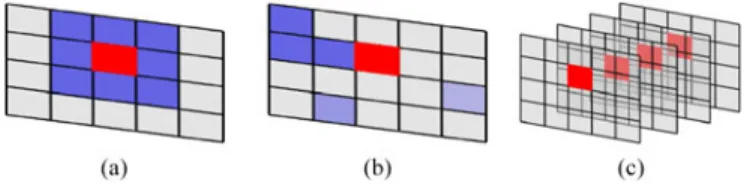
If the estimation of the covariance matrix ˜Γ is made through a boxcar filtering, the pixelsk are chosen in the neighborhood of the pixel of interest, as shown in Fig. 1(a). When ˜Γ is estimated temporally, the pixelsk are located in the same coordinates of the images contained in the temporal stack, i.e., after coregistra-tion of the different acquisicoregistra-tions. As we can see in Fig. 1(c), there are no spatial averaging involved in our temporal estimation of entropy.
The covariance matrix of a pixel can also be estimated using a sum of weighted covariance matrices:
˜Γ =!L
l=1
w(l)Tl (4)
where w(l) are the weights associated with each sample. This is done in the NL-SAR algorithm [5] in which the covariance matrices that are summed {T}l are not necessarily the
covari-ance matrices of neighboring pixels. The weight w is chosen according to distances between the patches centered on the pixels of interest: the more similar matrices of the patches are, the more the covariance matrices of the pixel is taken into ac-count in the averaging. This estimation process is illustrated in Fig. 1(b). An equivalent number of looks (ENL) can be
com-Fig. 1. Different process of estimation of the covariance matrix. (a) Boxcar estimation. (b) NL-SAR estimation. (c) Temporal estimation.
puted from the weights:
ENL=(" w(l))" 2
w(l)2 . (5) The ENL represents the factor of reduction of the variance performed by the algorithm. It can be interpreted as an equi-valent number of independent samples used in the averaging, without taking into account the effect of the zero-padding. In the implementation of NL-SAR provided in [5], the ENL is rounded to the closest integer between 0 and 255.
The covariance matrix can also be constructed using a tem-poral stack of monochannel images acquired in interferometric mode. In this case, the vectork contains the different responses of a resolution cell along the time axis. The extra-diagonal terms ˜Γi,j i̸= j are called interferometric coherence between the
images i and j. The degree of coherence ρi,j can be defined by
ρi,j = |˜
Γi,j|
# ˜Γi,i˜Γj,j
, i̸= j (6) which is an indicator of the phase stability between the acquisi-tions i and j.
The entropy can be computed from eigenvectors {λi} of the
covariance matrix C through the following equation: H =− N ! i=1 pilogN pi, pi = λi "N j =1λj . (7) With this definition, the entropy lies between 0 and 1. If only one component is needed to explain the covariance matrix, H is equal to 0, while it is equal to 1 if the powers of three uncorrelated channels is equal.
When H is estimated from ˜Γ, it becomes a measure of vari-ability among the pixels that have been used to compute the em-pirical covariance matrix. Indeed, the eigenvectors/eigenvalues decomposition of the empirical covariance matrix is the first step of the PCA. To keep H meaningful, all the pixels in the sample set have to come from the same homogeneous area.
The entropy is denoted Hboxcar when the covariance matrix
is estimated spatially using a boxcar filtering. If the covariance matrix is estimated through the NL-SAR algorithm, the resultant H will be denoted HNL-SAR. The parameter Htemporalcorresponds
to a covariance matrix estimated using a temporal stack. A high Hboxcaror HNL-SARmeans that there is a great spatial variability
for a given instant, whereas a high Htemporal means that the
scattering mechanisms change between the acquisitions, for a given resolution cell.
TABLE I
EIGHTMATRICESUSED TOILLUSTRATED THECAUSE OFMISESTIMATION
H α in¯ ◦ Class
C1 0.1 45.5 Z8: Mechanism with different HH and VV return
C2 0.25 75 Z7: Double bounce mechanism
C3 0.40 20 Z9: Surface scattering
C4 0.6 45 Z5: Dipole scattering with different orientation angle
C5 0.76 30 Z6: Prevailing surface scattering from a rough surface
C6 0.8 65 Z4: Double bounce mixed with other mechanisms
C7 0.94 54 Z2: Multiple mechanisms with no particular orientation
C8 0.92 70 Z1: Double bounce mixed with multiple mechanisms
Their expressions can be found in the Appendix.
III. REVIEW OF THECAUSES OFMISESTIMATION OF THEENTROPY
The value of H is very sensitive to the estimation process. It can be affected by various causes of misestimation.
Among these causes, a bias can be introduced for small sample sets. The mix of different pixels population impacts H as well as the thermal noise in low-signal-to-noise-ratio (SNR) areas. Finally, the correlation between samples induced by the zero-padding or the interferometric degree of coherence can modify the values of H.
These causes have already been studied through a Monte Carlo process [12], [13]. These articles consider only low mix-ing proportions and low degrees of coherence. We will complete the previous studies with different scenarios that are represen-tative of both spatial and temporal estimation: higher mixing proportion as well as correlation between samples that are more representative of the interferometric degree of coherence. These results will shed new light on the study over real data and avoid wrong interpretation of the scatterers’ behavior.
This study will be conducted using eight Hermitian semipositive matrices, randomly generated, representative of the eight possible classes in the initial Cloude and Pottier clas-sification [1]. The parameters of these matrices are given in the Table I, and their expressions can be found in the Appendix.
A. Number of Samples
The number of selected samples has an important impact on the estimation of H [13]–[16]. In this section, we summarize these results and illustrate them for the lowest number of pixels used for the estimation in Section IV. The mean entropy esti-mated with 3, 6, and 100 pixels has been calculated 100 times using a Monte Carlo process. Confidence intervals are reported in Table II. Histograms of the estimation of entropy samples are shown in Fig. 2.
Entropy is underestimated when a few pixels are used. The bias increases with the true value of H. More than 100 pixels can be needed to estimate H without bias. Fig. 2 also illustrates that the mode of these distributions is below the entropy true value. Nevertheless, this figure shows that some contrast can be preserved if H is always estimated with the same number of samples: if six samples are used, low, medium, and high entropy
TABLE II CONFIDENCEINTERVAL FORH
N H ⟨H ⟩ − 3σH ⟨H ⟩ ⟨H ⟩ + 3σH C3 3 0.40 0.28 0.28 0.29 C3 6 0.40 0.34 0.34 0.35 C3 100 0.40 0.39 0.39 0.39 C4 3 0.60 0.39 0.40 0.40 C4 6 0.60 0.50 0.50 0.50 C4 100 0.60 0.60 0.60 0.60 C8 3 0.92 0.56 0.56 0.56 C8 6 0.92 0.73 0.74 0.74 C8 100 0.92 0.91 0.91 0.91
The mean of H is denoted ⟨H ⟩ and its standard deviation is denoted σH.
Fig. 2. Histograms of the H values for matrices C3 (H = 0.4) C4 (H
= 0.6) andC8 (H = 0.91) . (a) Three samples. (b) Six samples.
(c) Hundred samples.
Fig. 3. H for mixed pixel populations or for a signal mixed with noise. (a) H for mixed pixel populations. (b) H in presence of thermal noise.
can still be differentiated even if the boundary of these classes is not the theoretical one found in [1].
B. Mix of Pixels From Different Populations and Influence of the Thermal Noise
When different homogeneous areas are mixed during the es-timation, H does not represent the variability of a particular speckle law but the variability introduced by the estimation. To our knowledge, there is no theorem on the eigenvalues and eigenvectors of the sum of Hermitian matrices. In order to illus-trate the effects of mixing, we compute the entropy of covariance matrices that are the sum of two different covariance matrices of Table I with different mixing proportions r. The estimated entropy can be seen in Fig. 3(a). The entropy of the mixed popu-lations can reach higher values than the entropies of the original
covariance matrices. Moreover, this increase in H seems to be higher if their original ¯α are very different. For example, the mix ofC1withC4that have both an alpha angle near 45◦has
a maximum entropy of 0.63 which is not much more than the 0.6 inital entropy ofC4. On the other hand, the mix ofC2with
C3 can reach 0.76, while the initial entropy is around 0.45 for
C3 and 0.25 forC2, but they have an ¯α angle of 20◦and 70◦,
respectively.
The influence of the thermal noise on H can be modeled as a mixing with the matrix of the noise. If the noise is decorrelated and white, N= σ2I
d, where Idis the identity matrix and σ2 the
power of the noise. This matrix has an entropy of 1.
The effect of the noise is quantified by the SNR in dB. In this experience, we define the SNR as the ratio between the power of the most energetic channel and the power of the noise. The result of this simulation can be seen in Fig. 3(b). As expected, the thermal noise increases the entropy of the whole signal. The log scale makes the curves begin with a plateau before rising, eventually reaching H = 1. The rise begins for higher SNR and the slop is bigger when the original entropy is lower.
C. Correlation Between Samples
A correlation between the samples used in the estimation can be introduced spatially by the zero-padding. Temporally, this correlation is expressed by the interferometric degree of coherence defined in (6).
To illustrate the effect of a constant correlation between sam-ples on H, we draw one vector from a speckle law of covariance matrixΥ: Υ = ⎡ ⎢ ⎢ ⎢ ⎢ ⎣ C R R ... R R C R ... R R R C ... R ... ... ... ... R R R ... C ⎤ ⎥ ⎥ ⎥ ⎥ ⎦. (8) The size ofΥ is MN × MN, with M being the number of temporal realizations and N the number of polarization chan-nels. The matrix R represents the interferometric correlation and can be defined as
Rn ,n′= √ρnρn′Cn ,n′. (9)
The M realizations of the speckle of the polarization channel n have the same the degree of coherence ρn ∈ [0, 1].
To model the evolution through time of correlation between the channels, we defineΛ as
Λ = ⎡ ⎢ ⎢ ⎢ ⎢ ⎢ ⎢ ⎣ C T(1, 2) T(1, 3) ... T(1, M ) T(2, 1) C T(2, 3) ... T(2, M ) T(3, 1) T(3, 2) C ... T(3, M ) ... ... ... ... T(M, 1) T(M, 2) T(M, 3) ... C ⎤ ⎥ ⎥ ⎥ ⎥ ⎥ ⎥ ⎦ (10) where T(m, m′) n ,n′ = √ρnρn′|m −m ′| Cn ,n′ (11)
where, for each polarization channel n, ρn ∈ [0, 1].
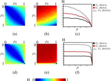
Fig. 4. Evolution of H with the correlation between samples. (a) H1 for
constant correlated samples. (b) H7for constant correlated samples. (c) Constant
ρ equal for all the polarizations. (d) H1 for decreasingly correlated samples.
(e) H7 for decreasingly correlated samples. (f) Decreasing ρ equal for all the
polarizations.
To keep the models simple, there is no phase difference between the acquisition.
We compute a mean entropy through a Monte Carlo process of 100 iterations. At each iteration, we draw a vector of MN = 300 components fromΥ or Λ. We decompose the vector in M = 100 scattering vectors of N = 3 components in order to compute the entropy of the sample set. In this simulation, ρ1 = ρ3and ρ2
range from 0 to 1. We obtain images of mean entropy that are represented in Fig. 4 for the matricesC1andC7, with a degree
of coherence that can be either constant [see Fig. 4(a) and (b)] or evolving through time [see Fig. 4(d) and (e)].
The diagonal of these images is the H value when all the polarization channels have the same degree of coherence. In the case of a constant degree of coherence, the non independence between samples decreases drastically the entropy, since the variability between the samples is lower. The underestimation is bigger for H closer to 1. The estimated value of an H of 0.9 is 0.5 if the correlation between the samples is 0.8, as shown in Fig. 4(c). Yet, this value of γ is common in interferometry over urban areas.
If the degree of coherence differs between the polarimetric channel, H can increase. The extreme case is when a polariza-tion channel is completely correlated, while the two other are completely independent. The extra-diagonal terms of the esti-mated covariance matrices involving the correlated polarization channel approach 0, leading to an increase of entropy. The final value of H depends on the initial covariance matrix. Since the correlation coefficient between the first and the second channel is 0.97 forC1, the decrease of this coefficient due to the
corre-lation of only the first or the second polarimetric channel leads to the high values that can be seen in Fig. 4(a).
The decrease of degree of coherence modeled by the matrix Λ limits the decrease in entropy due to the dependence be-tween samples. The influence of this non dependence becomes sensitive only for very high degree of coherence, as shown in
TABLE III
SUMMARY OF THEUSEDDATASETS
Area Sensor M Band δa δr Campaign
San Francisco UAVSAR 12 L 0.8 m 1.8 m San Francisco TerraSAR-X 3 X 6 m 2 m Amsterdam TerraSAR-X 3 X 6 m 2 m
Paracou SETHI 6 P 1.5 m 1.7 m TropiSAR Remmingstorp SETHI 3 P 0.85m 1m BioSAR-3
Fig. 4(f). The increase of H due to very nonuniform degree of coherence between polarimetric channels is exacerbated if the degree of coherence decreases through time.
D. Conclusion
In this section, we have shown that the entropy can be un-derestimated when too few samples are used in the estimation of the covariance matrix or when samples are correlated. The correlation of one polarization channel increases H, as the mix between two populations or in low-SNR areas. Nevertheless, these causes of misestimation do not have the same impact even if they have the same consequences.
1) The lack of samples to estimate H leads to an underes-timation of H, but with six samples, the contrast seems mostly preserved. Even though the value of entropy cannot be trusted when too few samples are used in the estimation process, a relative classification in high or low entropy can still be made.
2) The correlation between samples can have two distinct effects. If the degree of coherence is the same for all the polarization channels, H decreases with the correla-tion. This effect is lowered if the degree of coherence decreases with time. If the degree of coherence between two polarimetric channels is very dissimilar, H increases. This augmentation is exacerbated by the diminution of the correlation through time.
3) The mixing between population increases H. It is not pos-sible to differentiate homogeneous areas with high entropy from high entropy due to mixing. Thus, it is really diffi-cult to differentiate mixing occurring during the acquisi-tion process from mixing occurring during the estimaacquisi-tion process, leading to potentially wrong interpretation on the nature of the scatterers present on the scene.
4) The thermal noise increases H. It is a problem especially for areas with a very low signal and a very low entropy, such as water.
IV. COMPARISONBETWEENSPATIAL ANDTEMPORAL
ESTIMATION OF THEENTROPY
After reviewing the cause of misestimation of H, we can make an informed comparison between the different estimations of the covariance matrices on real data. The information about the datasets can be found in Table III. We choose datasets with various wavelengths and resolution, acquired over urban and natural areas.
TABLE IV
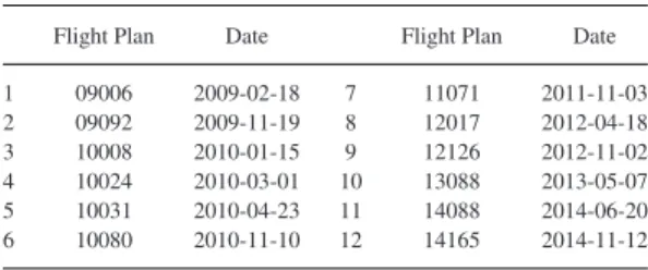
UAVSAR DATASETFLIGHTLINEHAYWRD_23501
Flight Plan Date Flight Plan Date 1 09006 2009-02-18 7 11071 2011-11-03 2 09092 2009-11-19 8 12017 2012-04-18 3 10008 2010-01-15 9 12126 2012-11-02 4 10024 2010-03-01 10 13088 2013-05-07 5 10031 2010-04-23 11 14088 2014-06-20 6 10080 2010-11-10 12 14165 2014-11-12 A. In Urban Areas
1) UAVSAR Images Over San Francisco: The comparison between spatial and temporal estimation of the entropy has been performed on 12 SLC full polarimetric L-band images acquired by UAVSAR, the JPL airborne system, over the city of San Francisco between 2009 and 2014. The list of the images can be found in the Table IV. The azimuth resolution is 0.8 m, while the range resolution is 1.8 m. The coregistration has been performed using the eFolki algorithm [6].
Given the large size of the original image, we focus on two extracts of these images. The first extract is centered on the SoMa (South of Market) district and highlights the effect of the building orientation. Indeed, San Francisco is composed of neighborhoods built following a grid plan with various orien-tations. In the configuration of these acquisitions, the buildings of the SoMa district are parallel to the trajectory of the sensor, which is not the case for the other neighborhoods. On the image in Pauli color shown in Fig. 5(a), we can see that the orienta-tion of the buildings changes their polarimetric behavior. The second extract is over Candlestick Point and shows various types of targets such as the ocean, a stadium, parking lots, a park, and some residential areas, as can be seen in Fig. 5(f).
Temporal entropy is computed on the 12 images. The spatial entropy is computed with a 3 pixels in range and 4 pixels in azimuth boxcar filter. The number of samples is thus the same for the two estimation methods. The images of the ENL show the number of pixels used in the NL-SAR algorithm.
The results are presented in Fig. 5. In this figure, we represent only Hboxcar and HNL-SAR for the first image of the temporal
stack. This choice is arbitrary since changes can occur in the temporal stack. In Fig. 6, two extreme Hboxcarare shown, as well
as the corresponding images. The main difference in Hboxcar
occurs over the sea: buildings, parks, and parkings have the same H level. The Pauli color images show that the images with the high backscattered signal lead to the lowest entropy. This increase in Hboxcarover the sea is probably due to the SNR
decrease.
Since there is a temporal change, Htemporalover the sea does
not represent the entropy of a unique kind of scatterers through the temporal stack but is the result of mixing. Its value is between the two extremes shown in Fig. 5 and higher than the Hboxcarof
the AIRSAR image [17]. We will thus focus on the other targets to compare Htemporal, Hboxcar, and HNL-SAR.
The Hboxcar map [see Fig. 5(d) and (i)] is very uniform. The
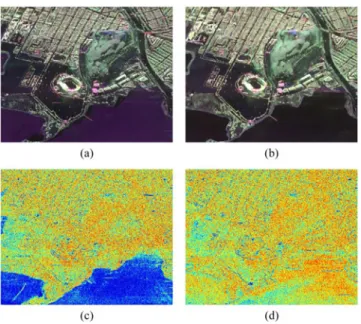
Fig. 5. San Francisco, extract over the SoMa District and Candlestick point, UAVSAR. The results for the boxcar and NL-SAR estimations are represented on the image acquired on February 18, 2009. (a) NL-SAR Pauli color: SoMa extract. (b) ENL: SoMa extract. (c) Htemporal: SoMa extract. (d) Hboxcar: SoMa extract.
(e) HNL-SAR: SoMa extract. (f) Pauli color NL-SAR: Candlestick extract. (g) ENL: Candlestick extract. (h) Htemporal: Candlestick extract. (i) Hboxcar: Candlestick
extract. (j) HNL-SAR: Candlestick extract.
Fig. 6. Extreme behavior of Hboxcarand the corresponding Pauli color images.
(a) Pauli color 2009-11-19. (b) Pauli color 2010-03-01. (c) Hboxcar2009-11-19.
(d) Hboxcar2010-03-01.
point-like scatterers have a low entropy. The uniform Hboxcarcan
be explained by the mixing introduced during the estimation. This mixing should be avoided for HNL-SAR, which is yet very
close to Hboxcar, as we can see in Fig. 5(e) and (j). However, the
aim of the NL-SAR algorithm is denoising. While computing ΓNL-SAR, the best pixels are chosen, but the algorithm chose
the configuration that maximizes the ENL. The ENL is often superior to the 12 samples used for Hboxcar since the median
ENL is 25.
The orientation of the targets seems to be the parameter that influences the most Hboxcar. The Hboxcar of highways winding
through the cities (Highway 80 and Highway 101) changes with their orientation even if the nature of the target does not change. Even if the map of HNL-SARis smoothed, the dependence in the
orientation of the targets remains, as illustrated in Fig. 5(j). Some classes can be discriminated using Htemporal, as shown
in Fig. 5(c) and (h): buildings have a lower Htemporal than the
bare soil like parking lots. Streets and the parks have the highest Htemporaland cannot be easily separated. Although the
orienta-tions of the scatterers affect also Htemporal, we can see that the
entropy of highways shows few variations on the image. The zero padding is approximately of 25% in azimuth and in range. Using a 3 × 4 window leads to 6.75 independent samples. A 4 × 5 window leads to 11.25 independent pixels and ensures a fair comparison between Hboxcarand Htemporal. The result can
be seen in Fig. 7(b). The Hboxcar 4 × 5 values are higher, but
their contrast is the same as for Hboxcar 3 × 4 represented in
Fig. 7(a).
Another way to increase the number of pixels could be spa-tiotemporal averaging. We performed such averaging on the SoMa extract: for each date, a 3 × 3 boxcar filtering yields co-variance matrices that are then averaged on the temporal axis. The result of the spatiotemporal averaging, zoomed at the bor-der of the SoMa district, can be found in Fig. 7(e). This extract shows that the advantage of Htemporal, i.e., a low entropy on
buildings independently of their orientation, is lost when a spa-tial averaging is processed. The Hspatiotemporalmap is admittedly
more contrasted that the Hboxcar, but it is less smooth than the
HNL-SARmap and less precise than Htemporal.
This dataset shows a high Hboxcarover urban areas that
com-plicate even a simple urban/non urban classification. The con-trast provided by the NL-SAR algorithm highlights mostly the orientation of neighborhood. Even if the value of Htemporalis
im-pacted by the orientation, the nature of the target is predominant on Htemporal.
Fig. 7. Comparison between boxcar, NLSAR, temporal, and spatiotemporal averaging. (a) Hboxcar3 × 4. (b) Hboxcar4 × 5. (c) HNL-SAR. (d) Htemporal.
(e) Hspatiotemporal.
Fig. 8. San Francisco, extract over the SoMa district, TerraSAR-X. The result for the boxcar and the NL-SAR estimations is illustrated on the image acquired on 2010-04-11. (a) Pauli NL-SAR. (b) ENL. (c) Htemporal. (d) Hboxcar1 × 3.
(e) Hboxcar5 × 5. (f) HNL-SAR.
2) TerraSAR-X Quad Pol Images Over San Francisco: For a closer look at the effects of the resolution on entropy, we com-pare the temporal, boxcar, and NL-SAR estimation of H over the SoMa district on TerraSAR-X images. The spatial resolu-tion is coarser than the UAVSAR resoluresolu-tion: it is around 6 m in azimuth and 2 m in range. The results are presented in Fig. 8.
Three images, acquired on 2010-04-11, 2010-04-22, and the 2010-04-03, were available. This is not the best configura-tion since H is drastically underestimated with three samples. Nevertheless, Htemporaland Hboxcarcomputed with three samples
follow the same tendencies, as shown in Fig. 8(c) and (d). Con-trary to H on the UAVSAR images, streets have a lower entropy
Fig. 9. Amsterdam, extract over the city center, TerraSAR-X. The result for the boxcar and the NL-SAR estimations are illustrated on the image acquired on 2010-04-21. (a) Pauli color. (b) ENL. (c) Htemporal. (d) Hboxcar 1 × 3.
(e) Hboxcar5 × 5. (f) HNL-SAR.
than building and H is lower on the SoMa district whose streets make a 37◦ angle with the trajectory than on other
neighbor-hoods yet aligned with the trajectory. This could be explained by the presence of high buildings of the SoMa districts, as seen in Fig. 8(a).
The tendencies of Hboxcar computed with three samples [see
Fig. 8(d)] are confirmed for Hboxcarcomputed with 25 samples
[see Fig. 8(e)] and for HNL-SAR[see Fig. 8(f)]. The areas with low
or high entropy remain the areas with low or high entropy. The augmentation of the sample set increases the contrast between low- and high-entropy areas and sharpens the edge of these areas when there is no mixing involved.
However, the medium Hboxcar 5 × 5 and the high HNL-SAR
over the buildings outside the SoMa districts is unexpected and highlights the impact of the resolution on the computation of H. The AIRSAR [17] or RADARSAT-2 [18] images showed a low entropy over buildings although H is close to 1 for this TerraSAR-X dataset or the UAVSAR dataset. The medium and uniform Hboxcaron the TerraSAR-X San Francisco images seems
induced by mixing during the estimation since streets are nearly not visible in Fig. 8(e), while they become visible with HNL-SAR
shown in Fig. 8(f).
A difference between mixing during acquisition and during estimation emerges. If a mechanism becomes dominant during the acquisition, H on this area will be low. This is the case when double bounce becomes the dominant scattering mechanism for buildings in coarse resolution image. On the other hand, mixing induced during the estimation can lead to a high H, since there is now variability in the sample set.
3) TerraSAR-X Quad Pol Images Over Amsterdam: The city of Amsterdam is built in concentric half circles around the train station, delimited by canals. The variation of the scat-tering mechanisms due to the variation of the orientation can be seen on the Pauli color image represented in Fig. 9(a).
We studied three Quad-Pol images acquired by TerraSAR-X in 2010-04-21, 2010-05-02, and 2010-05-13. The resolution of these images is 6 m in azimuth and 2 m in range. The results can be seen in Fig. 9.
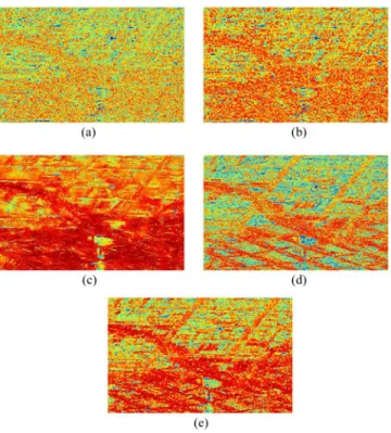
Fig. 10. TropiSAR dataset, Paracou images, extract containing the ground truth plots. The results for the boxcar and the NL-SAR estimations are shown on the image acquired on 2009-08-12. (a) Pauli color NL-SAR. (b) ENL. (c) Htemporal. (d) Hboxcar2 × 3. (e) HNL-SAR.
TABLE V
TROPISAR P-BANDTEMPORALDATASET
ID Date ID Date
1 0104 2009-08-12 4 0402 2009-08-24 2 0208 2009-08-14 5 0506 2009-08-30 3 0305 2009-08-17 6 0603 2009-09-01
The limitations caused by the low number of images in the temporal stack remain. As expected, Htemporal represented in
Fig. 9(c) is globally very low and shows poor contrast as Hboxcar
computed with three range pixels represented in Fig. 9(d). The tendencies of Hboxcarremain when 25 pixels are used, as shown
in Fig. 9(e). The contrast is sharper even if the entropy map is still very noisy. The noise is removed and the contrast is in-creased when an NL-SAR estimation of the covariance matrices is performed as we can see in Fig. 9(f).
On these images, the entropy is more influenced by the den-sity of the neighborhood than by their orientation. The ENL is represented in Fig. 9(b). It is low in high-entropy areas, showing that the scattering mechanisms are very different from one pixel to another.
This dataset shows again the difficulties of characterizing the urban areas in SAR. Depending on the resolution of the images, on their orientation and on the density of the neighborhoods, buildings can show very different scattering behavior and have a wide range of H.
B. In Natural Areas
1) TropiSAR Dataset: We tested the effects of the temporal estimation of the entropy on natural areas on images acquired in French Guiana in 2009. These images belong to the TropiSAR dataset acquired by ONERA with the airborne system SETHI. The images are listed in Table V. Their resolution is 1.5 m in azimuth and 1.7 m in range. We performed the test on an extract of the Paracou images, acquired at P-band on which ground truth of the biomass level was available. The information on these images is summarized in [19].
The covariance matrix is computed spatially using 3 pixels in azimut and 2 pixels in range. Only the first image is repre-sented in Fig. 10(d), because the values of Hboxcardid not change
through the temporal stack. The Htemporalmap is computed
tem-porally using the six temporal samples of the same pixel and represented in Fig. 10.
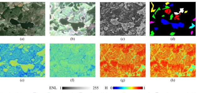
Fig. 11. Link between the entropies and physical parameters. (a) Htemporal.
(b) Hboxcar. (c) HNL-SAR. (d) Biomass (tons). (e) DEM (m).
The image [see Fig. 10(a)] can be divided in three parts: the first part is the pixels that have a high intensity due to their low incidence angle. The second part of the image is very hilly. The HV power is high and the image is very textured by the canopy. The last part is mostly constituted of flat land.
The values of Hboxcarare really high and show few contrasts:
95% of these values are over 0.5. As we can see in Fig. 10(d), there is still a spatial organization of these values: in the hilly parts of the image, Hboxcar is higher than on the flatter parts.
This behavior is kept for HNL-SAR, represented in Fig. 10(e).
Moreover, 95% of these values are over 0.7 even if the ENL represented in Fig. 10(b) is low compared to the other studied datasets.
The values of Htemporal are more contrasted than Hboxcar or
HNL-SAR values, but are difficult to explain. The comparison
with the biomass values provided with the images does not give any correlation. This comparison is done in Fig. 11 for the forest plot P16. We can notice that the spatial scale of these measures is very different: the variations of Htemporalare at a pixel level,
while the finest resolution of the biomass cells is 25 m × 25 m. The local elevation could also explain some Htemporalvariations
since the scattering mechanism variability could be increased by the landscape. To compare the variation of Htemporalwith the
landscape, we used the SRTM database. This DEM is repre-sented for the same forest plot as the biomass and Htemporal in
Fig. 11(e). Since it has a 90-m resolution, it is again very difficult to compare the elevation variation with the entropy variation, but Htemporalseems higher when the altitude increases.
Never-theless, a study with a more precise DEM should be conducted to draw more conclusions.
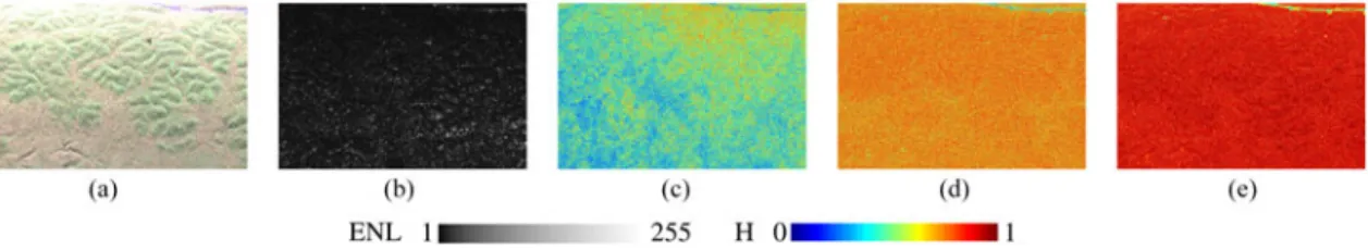
Fig. 12. Remningstorp, extract over the lake Acksj¨on, V¨asterg¨otland, Sweden. The results for the boxcar and the NL-SAR estimations are represented for the first image of the temporal stack. (a) Optical image. (b) Pauli color NL-SAR. (c) ENL. (d) Ground Truth. (e) Htemporal. (f) Hboxcar1 × 3. (g) Hboxcar5 × 5. (h)
HNL-SAR.
The spatial entropy over tropical forest is homogeneous and high when the number of looks increases. Indeed, their spatial organization makes the scattering mechanisms change from a pixel to another as expressed by the NL-SAR ENL. The temporal entropy shows a better contrast, but it is not well explained with the ground information that we have.
2) BioSAR Dataset: It contains three images acquired over the Remningstorp forest in Sweden. These images were acquired by ONERA, with the SETHI sensor, at P-band in 2010. The azimuth resolution is 0.85 m and the range resolution is 1 m. Various landscapes are present and the boreal forest has a very different structure than the tropical one.
We produced a ground truth for an extract of the image on which seven classes were distinguished: water, meadow with low grass, smooth meadow with high grass, textured meadow with high grass, meadow scattered with trees, forest, and dense forest. These classes are represented in Fig. 12(d).
The Htemporalmaps in Fig. 12(e) show four classes:
1) water: ⟨Htemporal⟩ ≈ 0.85;
2) meadows with low grass: ⟨Htemporal⟩ ≈ 0.5;
3) forests and dense forests, the textured meadows, meadows scattered with trees: ⟨Htemporal⟩ ≈ 0.35;
4) smooth meadows with high grass that have the lowest ⟨Htemporal⟩.
Only three classes can be separated with Hboxcar [see
Fig. 12(f)]:
1) water and meadows with low grass: ⟨Hboxcar⟩ ≈ 0.5;
2) smooth meadows: ⟨Hboxcar⟩ ≈ 0.3;
3) all the other areas that have a mean entropy around 0.4. Increasing the number of pixels in the boxcar estimation or the NL-SAR algorithm does not increase the separation capacities of Hboxcar, as we can see in Fig. 12(g) and (h) even if the
map is smoother. On the forest, small spots with low entropy appear on HNL-SAR. Our hypothesis is that these low-entropy
spots could come from the trunk response. Tree counting may become possible for boreal forest and long wavelength.
The ENL of the NL-SAR algorithm can be seen in Fig. 12(c). Homogeneous classes such as water and smooth meadow can be distinguished by their high ENL. Textured areas such as forest or meadow scattered with trees present a lower ENL.
Unlike tropical forest, boreal forest shows a contrasted H. Nevertheless, the discrimination between the different kinds of meadow or even between forest and meadow is difficult. A spatial criterion on the texture that can be extrapolated from the NL-SAR ENL seems more appropriate than a classification based on the H values.
V. LINKWITH THEINTERFEROMETRICCORRELATION
As we have seen in Section III-C, the correlation between samples can decrease the values of H, if all the polarization have the same correlation. Yet, the datasets that we have used to compare spatial and temporal entropy are acquired in interfero-metric conditions and can show a high degree of coherence. To study the link between the value of Htemporaland the
interfero-metric degree of coherence ρ, we focus on the UAVSAR dataset and the TropiSAR dataset, for which more than three images are available.
To compare more closely the link between the value of ρ and Htemporal, we draw, in Fig. 13, the degree of coherence
be-tween the first image and the other 11 images for six classes of scatterers that have different temporal behaviors, in the three polarization channels. These graphics show first that the degree of coherence is stable in time and has the same value in the three polarization channels. In this configuration, Htemporalis very
im-pacted by the value of the degree of coherence. When the degree of coherence is low, Htemporal can take all the possible values.
Fig. 13. Evolution of the degree of coherence with the first date for different targets.
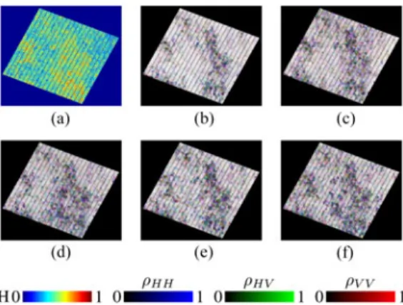
Fig. 14. Degree of coherence over the TropiSAR Paracou extract. (a) ρ 2009-08-12, 2009-08-14. (b) ρ 2009-2009-08-12, 2009-08-17.
that have low, a medium, and a high Htemporal, respectively. If
the degree of coherence increases, as for streets, buildings, and bright spots, the value of Htemporaldecreases.
For the TropiSAR dataset, the values of Htemporalwere
diffi-cult to explain. These images have a high degree of coherence because the acquisitions are separated only by two to six days. Moreover, the baselines are short to reduce the impact of the baseline decorrelation. But the degree of coherence evolves in time. In right upper corner of the image, the degree of coher-ence drops significantly between the first and the second ac-quisition and goes up again on the other images, as shown in Fig. 14. This figure shows a color composition of the degree of coherence in the three polarization channels. It underlines also that on high coherency areas, the degree of coherence does not change with the polarization channel, while there are more vari-ations in low-coherence areas. Htemporal is thus expected to be
higher in the right upper corner of the image, which is confirmed by Fig. 10(c).
This behavior is studied more closely over the forest plot P16 in Fig. 15. The degree of coherence shows variations with time and with the polarization channels. Nevertheless, the pixels with high Htemporal are pixels that have always a low degree
of coherence and the pixels with a constant high degree of coherence have a low entropy. But there is no clear correlation between the Htemporaland the degree of coherence values because
of the important variation in ρ.
The degree of coherence and Htemporalshares common
infor-mation. Even so they are not redundant. The value of Htemporal
can bring information on the scattering mechanism variation in low and medium degree of coherence areas. It can help us to
Fig. 15. Evolution of the interferometric degree of coherence for the ground truth plot 16. (a) Htemporal. (b) ρ 08-12, 08-14. (c) ρ 08-12, 08-17. (d) ρ 08-12,
08-24. (e) ρ 08-12, 08-30. (f) ρ 08-12, 09-01.
understand why the degree of coherence is low. The temporal entropy can also be seen as an overall degree of polarimetric coherence along the temporal stack.
VI. CONCLUSION
Entropy is a measure of the randomness of a homogeneous area. It is close to 0 if the target is deterministic: all the realizations of the speckle are equal for this target. If the different realizations of a speckle distribution have various scat-tering vectors, the entropy increases with the amount of possible scattering mechanisms.
The estimation entropy on an image depends heavily on the acquisition conditions. Simulations have enabled us to compare the effects of four causes of misestimation of H. A low num-ber of samples leads to an underestimation of H. Although this underestimation increases with the value of H, the contrast can be partially preserved, even with only 6 pixels. If increasing the number of samples leads to the mixing between homogeneous areas with different H, the entropy will increase and can become higher than the initial entropies, leading to wrong interpretation on the nature of the variability: the variability is not in the scat-tering mechanisms but in the estimation process. The thermal noise increases also the entropy of areas with a low backscat-tered signal and low entropy. Underestimation of entropy can also be caused by correlation between the samples, if the corre-lation is the same for all the polarization channels. In the case of polarization channels with a different degree of coherence, the decrease of entropy is lowered and happens for higher de-gree of coherence. In the extreme scenario of very correlated polarization channels while the other channels are very uncor-related, the entropy can even be increased by the discrepancy between the degrees of coherence.
The study conducted over real data of various wavelength and various resolution confirms that, for the studied datasets, a boxcar estimation yields homogeneous entropy maps due to the mixing of different scattering mechanisms during the esti-mation. An increase in the number of pixels leads to a higher entropy.
To limit the mixing between regions with different speckle distributions, advanced speckle filtering such as the NL-SAR
algorithm can be used. The entropy maps are smoothed, but en-tropy values remain high since the number of pixels used during the estimation is drastically increased to ensure denoising.
Since numerous temporal stacks of polarimetric images are now available, we have proposed to estimate temporally H. This estimation method preserves the resolution of the image and introduces more contrast between highly depolarizing media and man-made targets. To exploit temporal entropy, numerous acquisitions are needed. Three acquisitions are not enough for Htemporalto provide more information than a spatial estimation.
In urban areas, the spatial entropy is expected to be low, especially over buildings. With the increase of the resolution, this statement is no longer true. The impact of the wavelength is not significant to explain these high values since they are observed at L and X bands. However, the oritentation of the buildings have a great impact on entropy. Depending on the resolution and the type of construction, this effect varies. But on all our datasets, a contrast is induced by the orientation on the entropy maps. Temporal entropy is less impacted than spatial entropy even if the effects are still visible.
On the other hand, the contrast of Htemporalis influenced by
the interferometric degree of coherence or its evolution. If the degree of coherence is high, Htemporal will be low because the
variability of the sample set decreases. Temporal entropy pro-vides global information about the temporal stability of the scattering mechanism. This information cannot be derived only from the interferometric degree of coherence.
APPENDIX
C1 =
⎡ ⎢ ⎣
0.49 0.48e−i0.92 0.06ei0.31
0.48ei0.92 0.50 0.07ei0.50
0.06ei0.31 0.07e−i0.50 0.01
⎤ ⎥ ⎦ C2 = ⎡ ⎢ ⎣
0.08 0.19e−i0.14 0.02e−i0.50
0.19ei0.14 0.86 0.16 0.02ei0.50 0.16 0.06 ⎤ ⎥ ⎦ C3 = ⎡ ⎢ ⎣
0.84 0.08ei1.07 0.10e−i1.06
0.08e−i1.07 0.05 0.06e−i1.56
0.10ei1.06 0.06ei1.56 0.11
⎤ ⎥ ⎦ C4 = ⎡ ⎢ ⎣
0.50 0.19e−i0.68 0.15e−i0.98
0.19ei0.68 0.09 0.10e−i056
0.15ei0.98 0.10ei0.56 0.41
⎤ ⎥ ⎦ C5 = ⎡ ⎢ ⎣
0.68 0.03ei0.76 0.02ei0.05
0.03e−i0.76 0.15 0.01e−i0.81
0.02e−i0.05 0.01ei0.81 0.17
⎤ ⎥ ⎦ C6 = ⎡ ⎢ ⎣
0.19 0.17ei0.81 0.08e−i0.94
0.17e−i0.81 0.42 0.07ei1.19
0.08ei0.94 0.07e−i1.19 0.39
⎤ ⎥ ⎦ C7 = ⎡ ⎢ ⎣
0.37 0.08e−i0.83 0.03ei1.04
0.08ei0.83 0.20 0.04e−i1.50
0.03e−i1.04 0.04ei1.50 0.30
⎤ ⎥ ⎦ C8 = ⎡ ⎢ ⎣
0.18 0.03e−i1.16 0.02ei0.33
0.03ei1.16 0.34 0.07e−i0.90
0.02e−i0.33 0.07ei0.90 0.48
⎤ ⎥ ⎦.
The phases are in radian.
ACKNOWLEDGMENT
The authors would like to thank the JPL for the UAVSAR images over San Francisco, the DLR for the Quad-Pol images over San Francisco and Amsterdam (LAN2939), and ESA for the TropiSAR and BIOSAR-3 datasets.
REFERENCES
[1] S. R. Cloude and E. Pottier, “An entropy based classification scheme for land applications of polarimetric SAR,” IEEE Trans. Geosci. Remote Sens., vol. 35, no. 1, pp. 68–78, Jan. 1997.
[2] J.-S. Lee, M. R. Grunes, and G. D. Grandi, “Polarimetric SAR speckle filtering and its implication for classification,” IEEE Trans. Geosci. Remote Sens., vol. 37, no. 5, pp. 2363–2373, Sep. 1999.
[3] G. Vasile, E. Trouv´e, J.-S. Lee, and V. Buzuloiu, “Intensity-driven adaptive-neighborhood technique for polarimetric and interferomet-ric SAR parameters estimation,” IEEE Trans. Geosci. Remote Sens., vol. 44, no. 6, pp. 1609–1621, Jun. 2006.
[4] A. Alonso-Gonzalez, C. Lopez-Martinez, and P. Salembier, “Filtering and segmentation of polarimetric SAR data based on binary partition trees,” IEEE Trans. Geosci. Remote Sens., vol. 50, no. 2, pp. 593–605, Feb. 2012. [5] C.-A. Deledalle, L. Denis, F. Tupin, A. Reigber, and M. J¨ager, “NL-SAR: A unified non-local framework for resolution-preserving (Pol)(In)SAR denoising,” IEEE Trans. Geosci. Remote Sens., vol. 4, no. 53, pp. 2021– 2038, Apr. 2014.
[6] A. Plyer, E. Colin-Koeniguer, and F. Weissgerber, “A new coregistration algorithm for recent applications on urban SAR images,” IEEE Geosci. Remote Sens. Lett., vol. 12, no. 11, pp. 2198–2202, Nov. 2015. [7] J.-M. Nicolas et al., “A first comparison of Cosmo-Skymed and
TerraSAR-X data over Chamonix Mont-Blanc test-site,” in Proc. IEEE Int. Geosci. Remote Sens. Symp., 2012, p. 4141.
[8] I. Montero, C. Lopez, and F. Fabregas, “Temporal and incidence angle dependence of PolSAR data for agricultural land cover analysis and char-acterization,” presented at the 5th Int. Workshop Sci. Appl. Polarimetric SAR Interferometry Polarimetry, Frascati, Italy, 2011.
[9] F. Weissgerber, E. Colin-Koeniguer, N. Trouv´e, and J.-M. Nicolas, “Com-parison between spatial and temporal estimation of entropy on polarimet-ric SAR images,” in Proc. 8th Int. Workshop Anal. Multitemporal Remote Sens. Images., 2015, pp. 1–4.
[10] F. Cao et al., “Influence of speckle filtering of polarimetric SAR data on different classification methods,” in Proc. IEEE Int. Geosci. Remote Sens. Symp., 2011, pp. 1052–1055.
[11] J. W. Goodman, “Some fundamental properties of speckle,” J. Opt. Soc. Am., vol. 66, no. 11, pp. 1145–1150, 1976.
[12] J.-S. Lee, T. L. Ainsworth, and M. R. Grunes, “Monte carlo evaluation of multi-look effect on entropy/alpha/anisotropy parameters of polarimetric target decomposition,” in Proc. IEEE Int. Geosci. Remote Sens. Symp., 2006, pp. 52–55.
[13] J.-S. Lee, T. L. Ainsworth, J. P. Kelly, and C. Lopez-Martinez, “Evalu-ation and bias removal of multilook effect on entropy/alpha/anisotropy in polarimetric SAR decomposition,” IEEE Trans. Geosci. Remote Sens., vol. 46, no. 10, pp. 3039–3052, Oct. 2008.
[14] C. L´opez-Mart´ınez, E. Pottier, and S. R. Cloude, “Statistical assessment of eigenvector-based target decomposition theorems in radar polarimetry,” IEEE Trans. Geosci. Remote Sens., vol. 43, no. 9, pp. 2058–2074, Sep. 2005.
[15] C. L´opez-Mart´ınez, I. Hajnsek, E. Pottier, and X. Fabregas, “Polarimetric speckle noise effects in quantitative physical parameters retrieval,” IEE Proc. Radar, Sonar Navigation, vol. 153, no. 3, pp. 250–259, 2006. [16] J.-S. Lee, E. Pottier, and L. Ferro-famil, “Scattering-model-based speckle
filtering of polarimetric SAR data,” IEEE Trans. Geosci. Remote Sens., vol. 44, no. 1, pp. 176–187, Jan. 2006.
[17] J.-S. Lee, M. R. Grunes, T. L. Ainsworth, L.-J. Du, D. L. Schuler, and S. R. Cloude, “Unsupervised classification using polarimetric decompo-sition and the complex Wishart classifier,” IEEE Trans. Geosci. Remote Sens., vol. 37, no. 5, pp. 2249–2258, Sep. 1999.
[18] E. Colin-Koeniguer, F. Weissgerber, N. Trouv´e, and J. M. Nicolas, “Mul-titemporal polarimetric SAR images for urban areas,” in Proc. IEEE Int. Geosci. Remote Sens. Symp., Milano, Italy, 2015, pp. 231–234. [19] P. Dubois-Fernandez et al., “The TropiSAR airborne campaign in French
Guiana: Objectives, description, and observed temporal behavior of the backscatter signal,” IEEE Trans. Geosci. Remote Sens., vol. 50, no. 8, pp. 3228–3241, Aug. 2012.
Flora Weissgerber received the M.Sc. degree in
sig-nal and image processing from Centrale Marseille and Aix-Marseille Universit´e, Marseille, France, in 2013. She is currently working toward the Ph.D. de-gree with ONERA, the French Aerospace Lab and Telecom ParisTech, Paris, France.
Her research interests include remote sensing, multicomponent signal analysis, complex number statistics, and analysis of the phase distribution in the context of SAR images processing.
Elise Colin-Koeniguer was born in France on
November 15, 1979. She received jointly the Dipl.Ing. degree in electrical engineering from ´Ecole Sup´erieure d’´electricit´e (Sup´elec), Gif-Sur-Yvette, France, and the M.Sc. degree in theoretical physics from the University of Orsay (Paris XI), Orsay, France, in 2002, and the Ph.D. degree in remote sens-ing from the University of Paris VI, Paris, France, in 2005.
She then joined the Department of Electromag-netism and Radar, French Aerospace Laboratory (ONERA), Palaiseau, France. Since 2013, she has been with the Department of Modeling and Information Processing, ONERA, where her activities include image processing, radar, optical polarimetry, and investigation of video pro-cessing. She is also the Principal Investigator with ONERA, taking part in the European Space Agency project POLSARap for defining the key applications of polarimetry in urban areas.
Nicolas Trouv´e was born in France on February 8,
1985. He received the Master’s and Dipl.Ing. degrees in optical engineering from the Institut d’Optique Graduate School, ParisTech, Paris, France, in 2008, and the Ph.D. degree from the Ecole Polytechnique Graduate School, Palaiseau, France, in 2011.
Since then, he has been with the Electromagnetism and Radar Department, French Aerospace Laboratory (ONERA), Palaiseau. His research interests include polarimetric image processing, detection, and simu-lation tools for radar.
Jean-Marie Nicolas received the Master’s degree
from the Ecole Normale Superieure de Saint Cloud, Lyon, France, in 1979, and the Ph.D. degree in physics from the University of Paris XI, Paris, France, in 1982.
He was a Research Scientist with the Laboratoire d’Electronique Philips in medical imaging and was then with Thomson CSF in signal and image pro-cessing. He is currently a Professor with the Signal and Image Processing Department, Ecole Nationale Superieure des Telecommunications (Telecom Paris), Paris. His main research interests include radar imaging.