Wigner function and the one-sided flux

PHYSICAL REVIEW C VOLUME 29, NUMBER 3 MARCH 1984

Wigner function and

the

one-sided flux

C.

Gnucci and

Fl.

Stancu

Institut dePhysique B5,UniUersite de Liege, B-4000Liege 1, Belgium

I,'Received 10 June 1983)

We calculate the Wigner function ofthe one-body density ofasystem of32independent particles

moving intwo adjacent cubic boxes communicating through awindow. We discuss the applicability of the currently used definition of the classical analog ofthe one-sided flux obtained from the Wigner function,

NUCLEAR REACTIONS Wigner function forasimple quantum mechanical

model, nucleon exchange, static one-sided flux.

The static one-sided current isused as a measure

of

the dissipation rate produced by nucleon exchange between

colliding nuclei. ' In the simplest form

of

his model Swiatecki' assumes that the nucleons are exchanged via a

sharply defined window. Randrup has taken into

ac-count the diffuseness

of

the nuclear surface in the Thomas-Fermi model and applied the proximity concept

to derive the one-sided current as afunction

of

the separa-tion distance between nuclei. Within the same concept penetrability effects and temperature dependence have been considered.

Recently attempts to derive the one-sided current on a

more microscopic basis have been made. ' _These

calcula-tions have a quantum-mechanical input. They are based on the knowledge

of

the wave functions given by time-dependent or adiabatic time-dependent Hartree-Fock

calculations, from which the Wigner distribution function

f(r,

k,

t)

of

the one-body density can be constructed. Then the classical analog

of

the one-sided flux in the z direction is defined as

of

length

L

on each edge. They communicate through a window situated in the plane

z=0

and which extends from

x

=

—

w to

x

=

w and _{from y}

= —

(L/2)

toy

=L/2

The system is therefore symmetric with respect to refiec-tions through each coordinate. As the parity

~;=+1

(i

=x,

y, z)isconserved, the basis functions are

u„'(i)=

' 1/2 2 n;m. cos

i;

m.

;=+1,

_{n; odd} l l '_1/2 2

.

ni~

_.

L.

sin i m

=

—

1 nl even l (2)

g =u„~(y)

g

C~„u„"(x)u„*(z),

with

L„=L„=L

and

_L,

=

2L.

The total parity is

m

=a„m„m;

and the wave functions _lt~ defined inside the

volume occupied by the two cubes can be expanded in

terms

of

the basis set (2)

j+(r,

t)=

—f

d

kk,

f(r,

k,

t) .

Feldmeier has also defined a quantum mechanical

opera-tor for the one-sided current.

If

the flux is oriented in the

zdirection, the expectation value

of

this operator amounts

to

expression

(1).

In the present work we want to discuss the applicability

of Eq. (1).

This is related to the

fact

that, contrary to the classical distribution function, the Wigner function can have regions

of

negative values and make the quantity (1) negative. Insuch cases some care must betaken.

Vfe limit our discussion to the static case by using the simple three-dimensional quantum mechanical model in-troduced in

Ref.

10. This model can be briefly described as follows. We consider two adjacent hard-walled cubes

where n

=(n„,

n,)and

p=m.

„m,

The intermediate wall in which the window has been

created can be simulated by the following potential: V

=

A,5(z)0( i

x

~

—

w)

.

(4)

An alternative description has been given in

Ref.

10. The

Schrodinger equation with the potential (4) becomes the following matrix equation:

gl«n

E'+.

n—

+&a.

Ã'an

=o

n'

where

f2

2

2m

L2

and

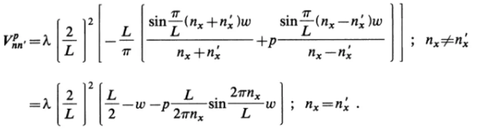
WIGNER FUNCTION AND THEONE-SIDED FLUX 869 2 2 1'nn

=~-L

slI1 (n»

+

n~)w

n„+n„'

~ 7T sin

—

(n„—

n„')IJ

+p

n

—

n' nxAnx 2&11

—

wW

—

_p

sin w

Thts expression holds for n, and n' odd th b i e

t(2)i

imp ies automatically1'

'

en'

=0

for n~

=

—

1 (8)

equivalent to C~

=5

1 o role in solvin

E

.

5

.

an an ne can notice that the va '

q. vj.ng

ewin ow as aconstant width 2w

which allowede the actorization

f

(3).

For

solvin cally one must truncat th

th i 1

tk

b

ae

esuminE. (5.

L

aue

a

enby

n in

t

he u cated space. even reduces to

X

odd due to (8).

For

N

d

as _{two p} ete e

c

oice

of

the range

of

A, and

t

with respect to

X

h

g o and the convergence ec o as been studied in

Ref.

10. As ample here we take

L

=4.

548 fmm and uI

=

=1

fm,

i.

i.

e.e., a,

wmdow about one third

of

the box sizi e, and solve

Eq.

(5) e m and

%=27.

Accor '

h I hiieve

t

he cancellation

of

th

h i di 11

The Wigner transforms orm

of

o ththe one-body density is

f(r,

k)=gf

(r,

k),

(9)

Xg

r

——

2 (10)

where

a

runs over all occu ie

and

a occupied states

of

both parities

~

x {fm) 0.5 ,1,0 I 0.5 {fm) 1.0

(a)

0.0 0.0

-0.5—

-0.

5 -1.

0—

0.0

-1.

0 0.0 N 1.5 -0.002— 0.0 0.

-2.

0—

0.0 -2.

0—

09 0.00025 I I I I I I I ~l

FIG.

1. (a) Contour plots forrthe intee ante rr ' ion of

I I I I t I I I I

g g a o o g

M

f

h 11 eso

fTb

a leI,multi liedb

or

870 C.GNUCCI AND

FI,

.

STANCU 29

Here we want tocalculate the one-sided flux at and per-pendicular to the window. Then the quantity

of

interest is

the Wigner function evaluated at z

=0

and integrated over the variables y,

k,

and k».

For

fixed o.

'and

_p let us call it

I

I'"(x,

k,

)=

f

dy

f"

dk„

f

dk»f»(r, k)

_~z ().

(11)

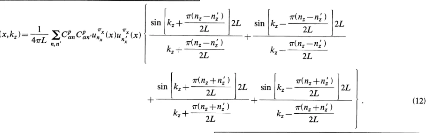
Carrying out the integrations we obtain:

F»(x,

k,

)=

QC»„C»„u„"(x)u,

"(x)

' m._(n, n—

,

'₎ sin

k+

2L 2L vr(n, n,'

)—

2L m(n,

—

n,

')

sin

k,

—

2L 2L 7r(n,

—

n,') 2L n._(n,

_+n,

'₎ sin k

+

2L 2L m._(n,

+n,

'₎

k,

+

2L vr(n,

_+n,

' ) sin

k,

—

2L 2L m._(n,

+n,

'₎

k,

—

2L (12)

At the window we define an average one-sided flux for

each state

e,

m.

(j )

~'"=

f

dx

j

dk,

k,

Fx(x,

_k,

),

(13)

where 2ujL isthe window area.

In a plane (x,

k,

)the function (12)has reflectional

sym-metry with respect to both variables. Therefore only one quarter

of

this plane needs to be used to represent it and

we have chosen the half axes

x

&

0

and

k,

&

0.

Throughout the whole

of

this work the values

of

X

and k

have been fixed as mentioned. Figure 1(a) shows contour plots

of

the function (12) for

a

=

1 and _p

=

1,

i.

e., the

lowest eigenvalue

of Eq.

(5). The variable

x

runs through the opening

of

the window

of

size uj

=

1fm, and ~

k,

~

ex-tends up to

2.

7 fm

', i.

e., well beyond the region where

the function ispractically zero. The contour plots show a

I

simple structure. The function is positive only for

~

k,

~

&0.

35 fm

'.

The integration over

x

and ~

k,

~ gives

roughly zero but the one-sided flux (1)results from the product

k,

F»~(x,

k,

)

=k,

F~~(x,

—

k,

)

with

k,

pO, which gives large weight to the negative

values

of

F» _{so that the average flux (13)turns out to be}

negative. The result isshown in Fig.2(a) and is associated

with state (1)or (4) from Table

I.

One can also see that these are not the only states which produce anegative flux at uj &1fm. Bytaking four orfive occupied states the to-tal flux remains negative, but the situation changes at larger w or when more states are occupied. The box size under consideration can accommodate 32 particles at den-sity

p=0.

17 fm . Then all eight states from Table

I

must be occupied, each being four times degenerate.

Sum-10— 2 O X P) C3 X 4— L/2 1 2 L/2 1 w Ifmj w {fmj

FIG.

2. (a)The partial average one-sided flux (13) as a function of(jj. Each curve gives four times the contribution ofone ofthe states indicated inTable

I.

(b)The total average one-sided flux as afunction ofwfor asystem of32 particles.

29 WIGNER FUNCTION AND THEONE-SIDED FLUX 871

TABLE

I.

The lowest eight states in increasing order for

E

for a box ofsize L

=4.

548fm and a window size ur

=1

fm. Equation (5)has been solved for 1V

=27

and A,

=10'

MeV frn. The columns

in-dicate the following: m;

—

the parity fori

=x,

y, z;o.

—

the eigenvalues E~of Eq.(5) inincreasing order,

2 e„~

=

—

ny 2m L and State

E

77

+1

+1

+1

+1

—

1

+1

—

1

+1

+1

+1

+1

—

1

+

1

—

1

+1

+1

17.60 19.80 40.71 17.60 49.40 19.80 49.50 49.50 9.90 9.90 9.90 39.60 9.90 39.60 9.90 9.90 27.50 29.70 50.61 57.20 59.30 59.40 59.40 59.40

ming up all the corresponding functions F~~ we obtain the result

of Fig.

1(b). The function has more structure and is positive in a large region, reaching a maximum at

~

k,

~

—

1.

15 fm

'.

Altogether this produces a positive average flux shown in Fig. 2(b). In detail this happens as follows: The total average flux is the sum

of

all partial contributions from

Fig.

2(a). The states with m,

= —

1 give rise to a positive flux at any w. One can see that at

small w there is almost a compensation for pairs

of

states, one with m.

,

=+1

_{and the other with m,}

= —

_{1, so that the}

flux remains small but positive. Around

w=l

fm the rise in the flux is dominated by the third occupied state, and beyond w

=

1 fm the positive contributions dominate. We

found that such a description holds for any N between 5 and 39 when A, takes a value in the range 10

—

10

MeVfm. In Fig. 2(b) the region

w&0.

6 fm has been omitted because

_X

=27

is not yet large enough to give a satisfactory cancellation

of

the wave function at the inter-mediate wall. As mentioned in

Ref.

10,at w

&0.

8fm we

must take N

~

39 forhaving such acondition fulfilled.

The conclusion we would like to draw is that some care

must be taken in using the definition (1)

of

the one-sided flux for a quantum system. When the number

of

occu-pied states is not large enough the result might be negative and the result does not have a meaning. But when the system contains asufficient number

of

particles the result can be interpreted as the classical analog

of

the one-sided flux. Adetailed analysis

of

the one-sided current resulting from other quantum-mechanical models might bring more insight into the problem.

We are indebted to

L.

Wilets for valuable comments and a critical reading

of

the manuscript. We are also grateful to W.

J.

Swiatecki, H. Feldmeier, and

G.

F.

Bertsch for instructive discussions. Thanks are due to

P.

Closset for computational help with the contour plots.

One

of

us

(C.

G.

) acknowledges financial support from the

Institut Interuniversitaire des Sciences Nucleaires.

W.

J.

Swiatecki,

J.

Phys. (Paris) 33,Suppl. No. 8-9,C5(1972).

2J. Qocki,

Y.

Boneh,

J.

R.

Nix,

J.

Randrup, M. Robel, A.

J.

Sierk, and W.

J.

Swiatecki, Ann. Phys. (N.

Y.

}113, 330 (1970}. 3J.Randrup, Ann. Phys. (N.

Y.

) 112, 356 (1978).

4C. M. Ko,

G.

F.

Bertsch, and

D.

Cha, Phys. Lett. 77B, 174

(1978).

5U.Brosaand

D.

H.

E.

Gross, Z.Phys. A298, 91 (1980).

Fl.Stancu and

D.

M.Brink, Phys. Rev.C25, 2450(1982).

7M. Prakash, S.Shlomo,

B. S.

Nilsson,

J.

P.Bondorf, and

F.

E.

Serr, Phys. Rev. Lett. 47,898 (1981);Nucl. Phys. A385,483

(1982}.

K.

Goeke,

F.

Griimmer, and P.-G. Reinhard, Ann. Phys. (N.

Y.

)(to bepublished); and private communication.

H. Feldmeier, Proceedings of the Workshop on Nuclear Dynamics, Lawrence Berkeley Laboratory Report

LBL-10688, UC-34C, CONF-800329, 1980.

C. Gnucci, Fl. Stancu, and L.Wilets, Phys. Lett. 127B, 10 (1983).