Science Arts & Métiers (SAM)
is an open access repository that collects the work of Arts et Métiers Institute of
Technology researchers and makes it freely available over the web where possible.
This is an author-deposited version published in: https://sam.ensam.eu
Handle ID: .http://hdl.handle.net/10985/15955
To cite this version :
Christophe PRADERE, L. CLERJAUD, Jean-Christophe BATSALE, S. DILHAIRE - High speed heterodyne infrared thermography applied to thermal diffusivity identification - Review of Scientific Instruments - Vol. 82, n°5, p.054901 - 2011
Any correspondence concerning this service should be sent to the repository Administrator : [email protected]
High speed heterodyne infrared thermography applied to thermal
diffusivity identification
C. Pradere,1,a)L. Clerjaud,1J. C. Batsale,1and S. Dilhaire2
1TREFLE Laboratory UMR 8508: CNRS-UB1-PARISTECH, Esplanade des Arts et Métiers,
33405 Talence, France
2LOMA UMR 5798: CNRS-UB1, 351 Cours de la Libération, 33405 Talence, Cedex, France (Received 8 October 2010; accepted 31 March 2011; published online 10 May 2011)
We have combined InfraRed thermography and thermal wave techniques to perform microscale, ul-trafast (microsecond) temperature field measurements. The method is based on an IR camera coupled to a microscope and synchronized to the heat source by means of phase locked function genera-tors. The principle is based on electronic stroboscopic sampling where the low IR camera acquisition frequency facq(25 Hz) undersamples a high frequency thermal wave. This technique permits the
mea-surement of the emissive thermal response at a (microsecond) short time scale (microsecond) with the full frame mode of the IR camera with a spatial thermal resolution of 7 µm. Then it becomes possible to study 3D transient heat transfer in heterogeneous and high thermal conductive thin layers. Thus it is possible for the first time in our knowledge to achieve temperature field measurements in hetero-geneous media within a wide range of time domains. The IR camera is now a suitable instrument for multiscale thermal analysis. © 2011 American Institute of Physics. [doi:10.1063/1.3581335]
I. INTRODUCTION
For years, two major techniques have been used to achieve small scale thermal imaging of heterogeneous mate-rials. The first category uses photoreflectance1–6 microscopy whereas the second applies InfraRed thermography.7–12 The major advantage of the first technique gives the possibility of working with spatial resolution close to 1 µm and thermal ex-citation frequencies higher than 1 MHz. Nevertheless, since the property involved in photoreflectance microscopy is the proportionality between the variation of the reflectivity and the variation of the temperature at the surface of the sample, the technique is better suited to high reflective materials. A CCD camera or a simple photodiode is used for the measure-ment of the reflected light.
The second technique uses an infrared camera for the direct measurement of the temperature of a material. Many studies7,8use pulsed thermography (PT), some other authors have exploited: lock-in or modulated thermography (MT)9 and pulsed phase thermography (PPT).10The comparison be-tween these methods is discussed here. We have just focused on their limitations especially the acquisition rate and the way it can be surpassed. Nowadays, the full frame acquisi-tion rate of the best IR camera is close to 200 Hz. It becomes very difficult to acquire high speed thermal phenomena with-out aliasing due to undersampling. This very low frequency acquisition is a drawback for the study of thin thermal conduc-tive materials where the characteristic diffusion time is very low (< 10 ms).
The idea presented in this paper is to combine infrared thermography with thermal wave techniques and electronic stroboscopic sampling2to acquire ultrafast temperature field with micrometric spatial resolution. First, a microscope is
a)Author to whom correspondence should be addressed. Electronic mail: [email protected].
associated with the IR camera to obtain a spatial resolution of 7 µm. This resolution is comparable to the spatial resolution of 1 µm obtained by photoreflectance techniques. Another ad-vantage of the IR camera is to perform direct measurements of the temperature on low reflective materials. The IR camera behaves as a contactless temperature sensor associated with a high frequency pulsed periodic thermal wave excitation, this allows the analysis of numerous materials in a wide frequency range especially good thermal conductors where classical IR thermography is limited by its low acquisition rate (100 Hz).
The aim of this paper is to present a new high speed IR thermal imaging technique applied to the determination of thermal diffusivity with a micrometric lateral resolution. First the experimental setup is described and the principle of the heterodyne IR thermography is detailed. Then, the first results obtained on high thermal conductive materials with pulsed periodic thermal generation are presented. The esti-mation of in-plane thermal diffusivity is performed on both isotropic and anisotropic homogeneous materials and finally, the capabilities of the technique are discussed.
II. EXPERIMENTAL SETUP
Figure1shows the scheme of the experimental setup. The thermal excitation is performed with a 1 W power laser diode at 830 nm wavelength. The diode is modulated by a first func-tion generator. This allows to achieve any periodic excitafunc-tion (pulsed or sine wave), for a frequency range up to 30 kHz only limited by the laser diode rising time. The laser diode function generator is phase locked with a second generator used to trigger the camera acquisition. Optical lenses are also used to focus the laser diode onto the sample. A dichroic mir-ror, with high reflectivity for visible and near IR light (from 400 to 1000 nm) and with high transparency for IR (95% transmission from 2 to 5 µm) wavelengths, is used to direct
054901-2 Pradereet al. Rev. Sci. Instrum. 82, 054901 (2011) x y Sample z Dichroic mirror Laser diode IR objective Beam IR emission IR Camera Low frequency
Acquisition signal generator (25 to 200 Hz)
Excitation signal generator (25 to 30 kHz)
10 MHz phase locked
Optical lens facq
fexc
FIG. 1. (Color online) Scheme of the experimental setup.
the laser beam onto the sample at the same time as the emit-ted IR light is direcemit-ted to an InSb (1.9 to 5.2 µm) IR camera. This camera is associated with an IR Germanium objective. The magnification factor of our IR imaging system goes from one to three. Since the camera sensor is a 256×256 pixels ar-ray with a 25 µm pitch, it enables to obtain spatial resolutions from 7 to 25 µm.
III. HETERODYNE SAMPLING WITH AN IR CAMERA
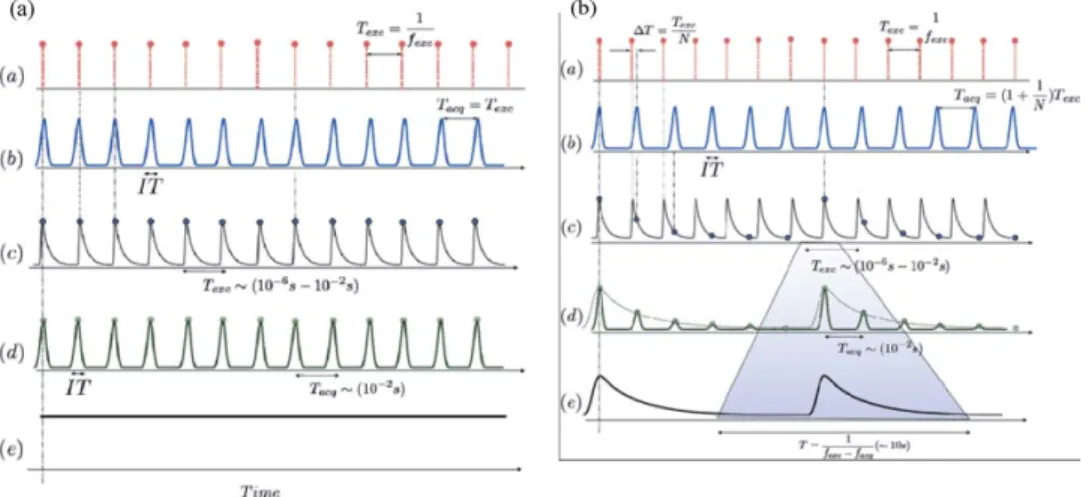
The principle of the method is explained through the two examples illustrated in Fig.2. The excitation signal [lines (a)] is represented by a Dirac comb at frequency fexc. This
exci-tation produces a thermal wave at the same frequency. The temperature response is represented in line (c) in both graphs. The ratio of the thermal wave excitation frequency fexc
and the IR camera acquisition rate facqis fixed to an integer
value k: fexc = kfacq. In that case, one can easily see that the
temperature is always sampled ≈ at the same time step and the resulting sampled signal is constant, see Fig.2(a)lines (d) and (e). Moreover, the whole signal can be sampled through a “stroboscopic” effect by slightly shifting the frequency
acqui-sition according to the following relation: fexc= (k + ε) facq,
with ε ≪ 1.
εcan be expressed by a fractional number 1/N, then the acquisition frequency can be expressed: fexc= (k + 1/N)facq,
where N becomes the number of points acquired by period. This is equivalent to having a linear variation of the phase shift between the acquisition and the excitation signals. Thus, the temperature response is then sampled with an equivalent "t that is expanded [see Fig. 2(b)]. The sampling time is equal and is expressed as follows:"t = texc/N, for k = 1.
For pedagogic reasons we have plotted the signal in Fig. 2 for k = 1.
The integration time (IT) of the IR camera has now to be taken into account for the frame acquisition. The typical value of IT is between 1 µs and 1 ms. This corresponds to the time needed by the camera to perform a snapshot. For the measured thermal response, the IT behaves as a low pass filter limiting the measurable maximum frequency. This main drawback appears as a rolling average on the resulting sampled signal. Thus, it becomes possible to follow any thermal phenomena at microsecond time scale. Depending on the level of the thermal signal, the IT is adjusted in order to optimize both SNR and temporal resolution. The actual temporal resolution is then given by the maximum between integration time and sampling period ("t).
IV. MEASUREMENTS WITH PERIODICALLY PULSED EXCITATION
Experimental results obtained with periodically pulsed excitation are presented in Fig.3. The sample under study is a 2 mm thick Silicon Carbide (SiC) layer with a diameter of 20 mm and a thermal diffusivity about 4.5 × 10⁻⁵m2s−1.
The pulse duration is 400 µs with a 150 Hz repetition rate. The peak power of the laser diode is 1 W over 400 µs, corresponding to the energy of 400 µJ focused on a 10 µm di-ameter spot. Assuming that the whole energy is absorbed by the sample, the density energy is closed to 5 MJ m−2. We have
fixed the acquisition frequency facq= 75 Hz, the number of
points per period N = 4000 corresponding to a sampling time
FIG. 2. (Color online) Illustration of the heterodyne sampling: a) case of a pulsed periodic signal with facq= fexc, b) case of a pulsed periodic signal with non
integer ratio between fexc= (1+1/N)facq. Line (a) corresponds to the excitation signal, line (b) to the acquisition synchro trigger of with an integration time (IT),
FIG. 3. (Color online) Measured temperature fields for periodic pulsed flash at f = 150 Hz: (a) just after the pulse (b) during the thermal relaxation at
t = 200 µs.
FIG. 4. (Color online) Log–Log representation of the spatial average (along x and y directions) of the measured temperature field.
Semi-infinite in z direction boundary condition z x y Semi-infinite in x direction boundary condition Semi-infinite in y direction boundary condition
Spatial and temporal Dirac thermal solicitation
ax
az
ay
FIG. 5. (Color online) Schema of the 3D transient system with semi-infinite boundary conditions and spatial and temporal Dirac thermal solicitation.
about 1.6 µs. The integration time is 200 µs. The acquisi-tion time is 50 s. The temperature relaxaacquisi-tion fields are shown in Figs.3(a)and3(b), respectively, just after the laser pulse (t = 0+) and for t = 200 µs.
We have plotted in a log–log scale the spatial average value (along x and y directions) as a function of time (Fig.4). One can easily see, the −1/2 slope corresponding to the semi-infinite behavior of the material between 200 µs to 1 ms.
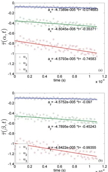
FIG. 6. (Color online) Normalized temperature vs time for the first three Fourier components: (a) in x direction and (b) in y direction, solid line corre-spond to the fits performed with Eqs.(8)and(9).
054901-4 Pradereet al. Rev. Sci. Instrum. 82, 054901 (2011)
The sampling time is close to 1.6 µs. The semi-infinite behav-ior (slope −1/2) is observed during 650 time steps of the film. The 200 µs integration time (see Fig.6) leads to not having to consider the points before IT for the physical interpretation of the data. The last point concerns the boundary condition (see Fig.4). The thermal wave penetration depth strongly de-pends on the excitation frequency e =√a/π fexc. The thermal
characteristic time is classically defined by tc= e2/a. For our experimental conditions: 2 mm thickness, ther-mal diffusivity a = 4.5 × 10⁻⁵ m2s−1, and a thermal wave
frequency of 150 Hz, the propagation length is estimated at 400 µm. The propagation length is shorter than the sam-ple thickness, which explains the rapid temperature drop (see Fig.4) at 2 ms.
V. THERMAL DIFFUSIVITY ESTIMATION A. Analytical solution
We model the sample by a homogeneous anisotropic semi-infinite medium, in which we calculate the Green func-tion of the temperature response (space and time Dirac response). The model is illustrated in Fig.5.
The system is thermally described by the following set of equations representing the heat propagation and the boundary conditions: ax∂2T(x, y, z, t) ∂x2 +ay ∂2T(x, y, z, t) ∂y2 +az ∂2T(x, y, z, t) ∂z2 =∂T (x, y, z, t) ∂t T(x, y, z, t =0)=0 −λx ∂T(x, y, z, t) ∂x ! ! ! ! x→−∞=0;−λ x ∂T(x, y, z, t) ∂x ! ! ! ! x→+∞=0 −λy ∂T(x, y, z, t) ∂y ! ! ! ! y→−∞=0;−λ y ∂T(x, y, z, t) ∂y ! ! ! ! y→+∞=0 −λz ∂T(x, y, z, t) ∂z ! ! ! !z=0= ϕ0δ(x, y, z =0, t) ; −λz ∂T(x, y, z, t) ∂z ! ! ! ! z→+∞= 0. (1) Here, ϕ0is the power density expressed in W m−2.
According to the semi-infinite behavior of such system, a temporal Laplace and a double spatial Fourier transforms are applied to the temperature fields. From this integral transform, the entire system Eq.(1)is rewritten as follows:
d2θ(α, β, z, p) dz2 − "a x azα 2 +aay z β2+ p az # θ(α, β, z, p) = 0 −λz dθ(α, β, z, p) dz ! ! ! ! z=0= ϕ 0K; −λz dθ(α, β, z, p) dz ! ! ! ! z→+∞= 0. (2)
FIG. 7. (Color online) Snapshot of the temperature field just after the exci-tation. The color temperature scale unit is digital level (DL).
From the boundary conditions, the general solution of Eq.(3)is given by θ(α, β, z, p) = ϕ0 λz$ ax az α2+ay az β2+ p az × exp " −z$ aax z α2+ay az β2+ p az # . (3) An inverse Laplace transform is applied to the Eq.(4):
τ(α, β, z, t) = q0 ρCp√πaztexp " − z 2 4azt #
× exp%−axα2t&exp%−ayβ2t&. (4) Here, q0is the energy density expressed in W m−2.
Finally, the double inverse Fourier transform is used to obtain the temperature as function of x, y, z, and t. As the solution is calculated in z = 0, the general solution of a semi-infinite anisotropic homogeneous media is obtained:
T(x, y, z = 0, t) = Q0 ρCp√πazt × exp " − x 2 4axt # √πa xt exp " − y 2 4ayt # √πa yt . (5)
B. Validation of the method in isotropic case
From Eq.(4), the temperature in Fourier space can be calculated along x Eq.(6)and y Eq.(7)directions:
τ(α, β = 0, z = 0, t) = q0
ρCp√πazt exp %
FIG. 8. (Color online) Normalized temperature for anisotropic material vs time for the first two Fourier components: (a) in x direction and (b) in y direction, solid line corresponds to the fits performed with Eqs.(8)and(9).
τ(α = 0, β, z = 0, t) = q0
ρCp√πazt exp %
−ayβ2t& (7) These relations can be divided by the mean temperature field obtained by fixing α = 0 and β = 0 in the Fourier space. This ratio allows us to obtain new relations expressed in a logarithm form and given by
log (τ (α, t)) = −axα2t with τ (α, t) = τ(α = 0, β = 0, z = 0, t)τ(α, β = 0, z = 0, t) , (8) log (τ (β, t)) = −axβ2t with τ (β, t) = τ(α = 0, β, z = 0, t) τ(α = 0, β = 0, z = 0, t). (9) From these two relations the logarithm of the normalized temperature for the first three Fourier spatial frequencies and versus time can be plotted (Fig.6). One can easily see a linear
evolution of first Fourier frequencies. From this behavior and according to relations [Eqs. (8) and (9), the thermal diffusivity in x and y directions can be estimated (Fig.6) with good accuracy.
The estimated thermal diffusivities (averaged values for the three Fourier frequencies) are along x (4.71 × 10⁻⁵ m2s−1) and y (4.73 × 10⁻⁵m2s−1) directions. These
values confirm the isotropic assumption of the sample. This behavior is in very good agreement with the value of 4.5 × 10⁻⁵ m2s−1 for the thermal diffusivity found in the
liter-ature.
C. Application to anisotropic material
In this application, a polymeric material with glass fibres is tested. Here, the fibres are injected according to the y direc-tion and with a volumic ratio of 20%. The idea is to measure the in-plane thermal diffusivities to check the link between the anisotropic thermal properties and the percentage of fibres in the polymeric matrix. Figure7shows a snapshot of the mea-sured temperature field just after the excitation pulse.
The temperature image clearly shows the anisotropy of the material in the vertical direction in Fig.7. This is a direct consequence of the larger thermal diffusion in the y direction with respect to the x direction. By using the same estimation method (see Sec.V B), the thermal diffusivities are estimated (see Fig.8) for the two first Fourier frequencies.
The averaged values are along x (3.04 × 10⁻⁷ m2s−1)
and y (3.70 × 10⁻⁷m2s−1). The ratio of the two thermal
dif-fusivities in y and x directions is ay/ax = 1.22. This value shows a thermal diffusivity in y direction 22% much higher than the one in x direction. This value of 22% is in excellent agreement with the fibre volumetric ratio of 20%.
VI. CONCLUSION
We have demonstrated that heterodyne sampling tech-nique applied to high frequency temperature field acquisition is possible with a classical IR camera.
The time resolution of the technique is not limited by the acquisition frequency of the frame grabber, but only led by the integration time of the camera. This links the time resolution to the signal to noise ratio of the experiment. For a good signal to noise ratio one can use the shortest integration time of the camera. In our case this technique is a very promising high-speed tool for the exploration of thermal phenomena at a very short time scale (1 µs best time resolution).
From these first experimental results, an analytical thermal analysis was implemented for in-plane quantitative estimation of thermal diffusivity of homogeneous high con-ductive materials and low concon-ductive anisotropic material. This technique gives rise to new multiscale (time and space) research fields in thermal characterization of materials.
1J. Opsal, A. Rosencwaig, and D. L. Wilenborg,Appl. Opt. 22, 3169,
(1983).
2S. Grauby, B. C. Forget, S. Hole, and D. Fournier,Rev. Sci. Instrum.
054901-6 Pradereet al. Rev. Sci. Instrum. 82, 054901 (2011)
3S. Dilhaire, S. Grauby, and W. Claeys,Appl. Phys. Lett.84, 822 (2004). 4G. Pernot, M. Stoffel, I. Savic, F. Pezzoli, P. Chen, G. Savelli, A. Jacquot,
J. Schumann, U. Denker, I. Mönch, Ch. Deneke, O. G. Schmidt, J. M. Rampnoux, S. Wang, M. Plissonnier, A. Rastelli, S. Dilhaire, and N. Mingo,Nature Mater.9, 491 (2010).
5D. Rochais, H. Le Houëdec, F. Enguehard, J. Jumel, and F. Lepoutre,
J. Phys. D: Appl. Phys.38, 1498 (2005).
6A. Rosencwaig and G. BusseAppl. Phys. Lett.36, 725 (1980).
7D. L. Balageas, J.-C. Krapez, and P. Cielo,J. Appl. Phys. 59(2) 348
(1986).
8D. L. Balageas, A. A. Deem, and D. M. Bosher, Mater. Eval. 45(4) 461
(1987).
9G. Busse, D. Wu, and W. Karpen,J.Appl. Phys. 71(8), 3962 (1992). 10X. Maldague and S. Marinetti,J Appl. Phys79(5), 2694 (1996). 11G. M. Giovanni and C. Meola,NDT & E Int.35(8), 559 (2002). 12L. Clerjaud, C. Pradere, J. C. Batsale, and S. Dilhaire, “Heterodyne method
with an infrared camera for the thermal diffusivity estimation with periodic local heating in large range of frequencies (25 Hz to upper than 1 kHz),”
Quantitative InfraRed Thermography(Lavoisier, Cachan, France, 2010), Vol. 7, pp. 115–128.