Science Arts & Métiers (SAM)
is an open access repository that collects the work of Arts et Métiers Institute of
Technology researchers and makes it freely available over the web where possible.
This is an author-deposited version published in:
https://sam.ensam.eu
Handle ID: .
http://hdl.handle.net/10985/9870
To cite this version :
Anne BOMONT-ARZUR, Mario CONFENTE, Emmanuel SCHNEIDER, Olivier BOMONT,
Christophe LESCALIER, Anne BOMONT-ARZUR - Super High Strength Steel for automotive
applications - In: Seventh International Conference on High Speed Machining, Allemagne,
2008-05-28 - Seventh International Conference on High Speed Machining - 2008
Any correspondence concerning this service should be sent to the repository
Administrator :
archiveouverte@ensam.eu
Seventh International Conference on HIGH SPEED MACHINING 2008
Super High Strength Steels for automotive applications
Machinability in dry carbide drilling
A. Bomont-Arzur1, M. Confente1, E. Schneider2, O. Bomont2, C. Lescalier2
1
ArcelorMittal Gandrange R&D - Long Carbon Bars & Wires, Amnéville, France
2
Arts et Métiers ParisTech – Centre de Metz, Metz, France
Abstract
Intensive weight savings and out-sizing programs are developed in automotive industry and lead to increase the mechanical properties of the material of the automotive parts. ArcelorMittal has developed specific steel grades known as Super High Strength Steels which are designed for both high ductility and toughness and fatigue resistance. This paper investigates machinability for a drilling operation using an experimental methodology. One of the materials is a new low bainitic steel grade. Experiments are performed with a coated carbide solid drill. Thrust force and torque measurements, chip morphology analysis, surface quality monitoring and tool wear tests are carried out. Experiments are performed with and without lubricant.
Keywords:
Machinability, Drilling, Couple Tool-Material, Tool wear
1 INTRODUCTION
ArcelorMittal Gandrange R&D focuses on the
development of new steel grades involving metallurgical solutions designed on one hand to decrease the material raw cost and and on the other hand to improve both mechanical properties and formability within a whole manufacturing process involving forging and heat treatment and then machining [1] [2].
The most advanced steel grades are the so called "Super High Strength Steels" whose improvement in the manufacturing process efficiency should not be to the detriment of the mechanical properties which are crucial.
Many machining processes have already been
investigated: turning, drilling, gun drilling, gear hobbing [1] [2] [3] [4] [5]. This paper proposes some results concerned with drilling using a standardized method [6]. Literature proposes numerous studies devoted to drilling. Most of them are concerned with mechanistic modelling [7], tool geometry [7] [8], tool coating [8], tool wear [9] [10] [11]. Few papers are dealing with the influence of metallurgical solution on machinability. This paper tends to highlight the impact of the composition on the machinability when drilling with a carbide coated drill.
2 STEEL GRADES INVESTIGATED
Machinability is investigated for two different ArcelorMittal Super High Strength Steel grades called G and N. G and N are designed for both forging and machining application. The high formability level requires a low concentration in sulphur in order to prevent forming damages. The metallurgical machinability enhancement treatments currently performed (using sulphurs to lower friction level) should then be avoided. Machinability should then be investigated.
G and N metallurgical structures are different even if both steels should be regarded as low carbon steels. G structure is ferrito-pearlitic while N structure is bainitic. It is required by the high mechanical characteristics expected and is only due to the chemical composition and the cooling after hot rolling.
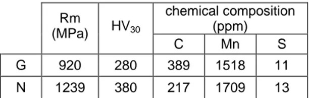
The main chemical composition and indicative mechanical properties are listed in the Table 1.
chemical composition (ppm) Rm (MPa) HV30 C Mn S G 920 280 389 1518 11 N 1239 380 217 1709 13
Table 1 : Steel grades indicative composition
3 THE COUPLE TOOL MATERIAL
The Couple Tool Material methodology is a standardized experimental protocol devoted to characterize the machinability. Experiments are to be done for each association work piece / cutting tool / machining operation. The result is an operating range, the whole acceptable machining conditions for that association. A machining condition is regarded as acceptable when:
• specific energy values are acceptable,
• chips are regular and fragmented,
• tool wear is regular and controllable,
• surface roughness and surface quality (i.e. hole roundness) are compatible with other similar machining applications,
3.1 Vcmin – fmin
The Couple Tool Material standard proposes to measure both the drilling torque and the thrust force and to determine the operating range from their variations versus either the cutting speed Vc or the feed f. The most convenient system for this purpose is a Kistler piezoelectric dynamometer.
The operating range is determined not from the global specific energy but from close physical quantities: the specific cutting pressures kcMz and kcFz calculated from
drilling torque and thrust force. Two sets of experiments are planned:
• at variable cutting speed,
• at variable feed.
A usual value of feed is arbitrarily chosen. The cutting speed varies within a large range. kcMZ and kcFz values
f D Mz 80 kc 2 drill Mz × × = (1) f D Fz kc drill Fz × = (2)
The curves kcMz = f(Vc) and kcFz = f(Vc) are drawn. Vcmin,
the minimal cutting speed which is allowed, is then deduced from their analysis. Vcmin is the value required to
ideally obtain low and constant values of kc Mz and kc Fz.
Power consumed during a drilling operation is easily calculated from the experimental values of drilling torque and thrust force using:
Qw u Vz Fz z Mz Pc= ×ω + × = × (3)
Experimental results analysis usually shows:
Vz Fz z
Mz×ω >> × (4)
Drilling power estimation is then:
Qw u z Mz
Pc≈ ×ω ≈ × (5)
The specific energy mainly depends on drilling torque rather on thrust force. A basic approach of machinability in drilling should also neglect the influence of thrust force. One more specific requirement of drilling is the correct chips evacuation especially for dry drilling operations where no cutting fluid helps chips to move along the flutes. One solution is to favour drilling conditions where short chips are produced.
3.2 Tool wear
Physical phenomena in tool wear (adhesion, abrasion, oxidation, diffusion) lead to an alteration of the tool geometry, and then to a perturbation of the machined parts geometry. The E 66-520 standard details how to identify the different tool wear patterns and characterize this geometry damages using some geometric quantities. Different attempts are performed there: evolution of VB measured on the relief face, evolution of wear zones area. The steel grades machinability is then compared through the tool life (T) or length being drilled until a VB value about 0.1 mm is reached.
Four different drilling conditions are arbitrarily chosen from the operating range for the wear tests of each steel grade and the lengths drilled are computed.
European standard proposes a tool life model taking into account both drilling conditions and geometric features of the hole being drilled, i.e. the length to diameter ratio.
C D l f T Vc 3 2 1 n drill drilled n n = × × × (6)
Machinability is investigated for one single tool and single hole depth. Tool life model could so be simplified:
1 3 1 2 1 1 n n drill drilled n n n 1 n 1 D l f Vc C T − − − × × × = (7) With f Vc 1000 L D T drill × × × × = π (8) And so drill n n drill drilled n n 1 n 1 1 D 1 D l f Vc ' C L 1 3 1 2 1 × × × × = − − − (9)
ldrilled / Ddrill and Ddrill are constant, therefore: 2 1 p p f Vc ' ' C L= × × (10) where p1, p2 and C'' are supposed to be constants for a
given couple tool / material.
4 EXPERIMENTAL DEVICE
The tool is a Titex A1164 TiN solid carbide drill used for short hole drilling (hole depths lower than three times the tool diameter). The cutting tool material is a K30 micrograin carbide. The drill is provided with a TiN coating for universal applications. The point angle is 140°.
Figure 1 : The tool employed Machining experiments are performed using:
• a 3-axis NC milling machine Somab Univer to determine the operating range,
• a 4-axis NC machining centre Ernault FH 45 for the wear tests.
Two specific workholding devices are designed and manufactured for both the operating range determination and the wear tests. The first one is a collet chuck mounted on a 9272 Kistler table used to measure both drilling forces and torque.
part collet chuck protection plate part collet chuck protection plate Titex twist drill part workholding system Kistler© 9272 dynamometer Titex twist drill part workholding system Kistler© 9272 dynamometer
Figure 2: Work holding device for force measurement tests
The second workholding system is located on a clamping cube. A tool life test in drilling generally induces several thousands of holes especially with low cutting speed and feed and consumes a huge global length of steel bars. The 4-axis machining centre and the clamping cube and the pallet changing system are particularly convenient. A whole set of clamps is then mounted on the four faces of the clamping cube. Eight 350 mm long steel bars are clamped enabling to drill almost 650 holes. The bars are first faced.
Figure 3: Work holding device for tool wear tests
5 EXPERIMENTS AND RESULTS
A data acquisition system records drilling torque Mz and thrust force Fz and radial forces (forces acting on the work piece in the plane perpendicular to the drilling direction). The radial forces values enable to detect an excessive run out or a poor regrinding or a tool deflection. The sampling rate is higher than the rotating speed and enables to get at least 2500 values during the drilling operation. A typical experimental curve is shown below:
-500 0 500 1 000 1 500 2 000 2 500 0 0.5 1 1.5 2 time (s) F o rc e ( N ) - M o m e n t (N .c m ) i Mz Fz Fy Fx
Figure 4: Force and torque measurements N - Vc = 70 m/min - f = 0.25 mm/rev - dry
This curve shows three consecutive stages: the tool engagement (0.4 s to 0.8 s), the tool progression (0.8 s to 1.7 s), and the tool withdrawal (1.7 s to 2 s).
The second stage occurs when the cutting lips are fully engaged in the work piece. Different trends are shown depending on the material and the drilling conditions: an almost constant level with more or less intensive fluctuations or a more or less slight increase in drilling torque Mz and thrust force Fz during tool progression. When it occurs, the tendency is usually linear. This can be due to the chip excavation the difficulty of which increases with depth. All the recorded data are analysed to get the mean value of Mz and Fz, the slope of the least square line based on Mz and Fz values. Confidence intervals are also calculated.
When the tool is withdrawing, the torque Mz is not negligible as expected. It may even reach levels similar to those measured while drilling. The highest value observed is about half the mean drilling torque. Chip evacuation difficulty is the more realistic reason nevertheless no chip clogging has been noticed during tests.
The radial forces are negligible. One notices that the variations are higher when the variations of the other channels are higher. Vibrations induced by the cutting (chip friction) have then an impact on the instantaneous axis-equilibrium of the tool.
5.1 Carbide-tool drilling force experiments
Since the drilling conditions range is extremely wide for a solid carbide coated tool, a protocol based on the standard is arbitrarily chosen to determine both Vcmin and
fmin.
All the experimental values, kcMz and kcFz, are plotted,
tendency curves are drawn which often show a horizontal asymptote for high cutting speed or feed values. Two lines are drawn:
• a tangent to the curve at the lowest value of cutting speed and feed,
• a horizontal asymptote at the high value.
The abscissa of the intersection point between these two lines is calculated. Vcmin and fmin are arbitrarily chosen
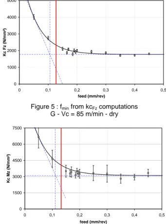
20% higher. Finer values are evaluated through applying statistical methods. This method seems more repeatable and so more reliable since it prevents interpretation errors. 0 1000 2000 3000 4000 5000 0 0,1 0,2 0,3 0,4 0,5 feed (mm/rev) K c F z ( N /m m ²)
Figure 5: fmin from kcFz computations
G - Vc = 85 m/min - dry 0 1500 3000 4500 6000 7500 0 0,1 0,2 0,3 0,4 0,5 feed (mm/rev) K c M z ( N /m m ²)
Figure 6: fmin from kcMz computations
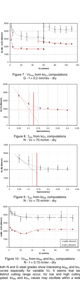
0 1000 2000 3000 4000 5000 0 20 40 60 80 100 120 Vc (m/min) K c M z k c F z ( N /m m ²)
Figure 7: Vcmin from kcFz computations
G - f = 0,2 mm/rev - dry 0 1000 2000 3000 4000 5000 0 0,05 0,1 0,15 0,2 0,25 0,3 0,35 feed (mm/rev) K c F z ( N /m m ²)
Figure 8: fmin from kcFz computations
N - Vc = 70 m/min - dry 0 1500 3000 4500 6000 7500 0 0,05 0,1 0,15 0,2 0,25 0,3 0,35 feed (mm/rev) K c M z ( N /m m ²)
Figure 9: fmin from kcMz computations
N - Vc = 70 m/min - dry 0 1000 2000 3000 4000 5000 0 20 40 60 80 100 120 Vc (m/min) k c M z k c F z ( N /m m ²) kcMz (N/mm²) kcFz (N/mm²)
Figure 10: Vcmin from kcMz and kcFz computations
N - f = 0,15 m/rev - dry
Both N and G steel grades show interesting kcMz and kcFz
curves especially for variable Vc. It seems that two distinct cutting range occur, for low and high cutting speed. kcMz and kcFz values may oscillate within a wide
interval (see Figure 7). In this particular case, experiment has been carried out several times with the same conditions (tool, workpiece).
Therefore two minimum cutting speed values Vcmin may
be defined. For productivity reasons the higher value is chosen and following tests are performed for both G and N with the higher cutting speeds allowed. Such a phenomenon is often due to the activation of a metallurgical enhancement mechanism (i.e. built-up layer formation) however neither G nor N is likely to generate such a layer.
Roughness measurements are frequently used to confirm fmin and Vcmin experimental values based on cutting forces
analysis. All the parts are also split to measure roughness along the cylinder generatrice. Roughness is measured using a profilometer Mahr Perthometer PZK.
Mahr Perthometer (profilometer) workpiece Mahr Perthometer (profilometer) workpiece
Figure 11: Roughness measurement device Figure 12 shows the roughness measurements for the N steel grade. Roughness is usually assumed as independent of the cutting speed according to geometrical models. An increase in the cutting speed tends there to decrease both the average roughness Ra as well as the confidence interval. 0 1 2 3 4 5 0 20 40 60 80 100 120 Vc (m/min) R a ( µ m )
Figure 12: Roughness measurement
N - f = 0,2 mm/rev - dry
The roughness increases with the feed (Figure 13) which seems similar to former studies [12]. The roughness measurements with various feed make it possible to confirm minimum or maximum value of feed (fmin or fmax).
The maximum feed value is a very useful indicator because the feed is the main influent condition on the thrust force. Contrarily to the cutting speed which is often limited by the machine-tool characteristics, the feed is the parameter allowing high productivity. The limiting factors
are due to chip evacuation problems or excessive thrust force or rapid tool wear rate.
0 1 2 3 4 5 6 7 0 0,05 0,1 0,15 0,2 0,25 0,3 0,35 0,4 f (mm/rev) R a ( µ m )
Figure 13: Roughness measurement
N - Vc = 70 m/min - dry
5.2 Chip morphology analysis
To complete the information collected during the drilling, chips are collected and observed for each pair (Vc, f) investigated. The chips morphology - this term includes their length, shape, colour, regularity … - is standardized (NF E-66-505) [13]. Chips are required to be short (fragmented) to be properly ejected during the drilling operation. The shots are taken with the same scale: the width of each is 7 mm.
Figure 14: Chip morphology graph G steel grade 2 5 20 30 50 70 80 90 100 110 0,05 0,1 0,15 0,2 0,25 0,35 0,3 Vc (m/min) f (m m /r ev ) 2 5 20 30 50 70 80 90 100 110 0,05 0,1 0,15 0,2 0,25 0,35 0,3 Vc (m/min) f (m m /r ev )
Figure 15: Chip morphology graph N steel grade
Once again, the chips which are generated at low cutting speed confirm the choice of a high minimum cutting speed. At low cutting speeds, the thermo mechanical phenomena are not severe enough to ensure the
fragmentation of the chips. At the opposite, for high cutting speeds, the chip is hot (blue).
5.3 Conclusion on Vcmin and fmin tests
The synthesis is presented below.
Steel grade Vcmin
(m/min) kc Mz ref (N/mm²) kc Fz ref (N/mm²) G 85 3600 2000 N 60 3200 2000
Table 2 : Synthetic table of Vcmin Steel grade fmin (mm/rev) fmax (mm/rev)
G 0.11 0.30
N 0.11 0.25
Table 3 : Synthetic table of fmin and fmax
Globally, N steel grade seems to allow higher cutting speed and thus higher productivity thanks to lower specific cutting pressure and thus drilling torque and thrust force at same feed level. These results should be correlated with the tool wear tests before proposing a reliable machinability ranking.
Drilling feeds allowed are similar. The G steel grade offers a higher fmax value (20 % higher than the one estimated
for N steel grade). A wider operating range induces a much more interesting machinability, because the cutting conditions are less restrictively to be chosen.
Drilling torque and thrust force may be predicted within the cutting conditions range which has been determined using relations involving experimental constants. These constants depend on the workpiece material and the tool used and the lubricating conditions. The models which are currently used only depend on uncut chip thickness (i.e. feed in drilling) : Mz mc ref ref Mz Mz f f kc kc × = (11) Fz mc ref ref Fz Fz f f kc kc × = (12)
Linear regression easily provides experimental values for these constants which show the differences between the two steel grades in terms of machinability (Table 4).
Steel grade kcMz ref
(N/mm²) mc Mz
kcFz ref
(N/mm²) mc Fz
G 1200 -0.65 700 -0.60
N 2100 -0.30 1100 -0.40
Table 4 : Synthetic table of cutting force model constants
6 TOOL WEAR TESTS
Tool wear tests are performed within the drilling range determined through the previous tests. Four different drilling conditions are arbitrarily chosen and the tool wear is followed by observing the edge geometrical evolution. Flank face is observed during tool life using a microscope. Flank wear is measured through the wear area and the wear land width which is easily determined due to the prior regrinding of the drill. The entire relief face image is computed from 4 adjacent snapshots.
The edge of the drill used is not straight. Moreover the load on the tool is not constant along the cutting edge. Different wear processes may occur and the wear rate is variable along the cutting edge. That is why five length Non-acceptable
chips
Best chips
Vc (m/min) f (mm/rev)
measurements are done each time the drill is observed (Figure 16).
Therefore, the tool wear criterion is given by the one of the 5 measurements that wears the most.
Figure 16: Tool wear measurement
The tool wear observations are easy due to the colour difference between TiN coating and tool substrate.
Figure 17: Tool wear measurement
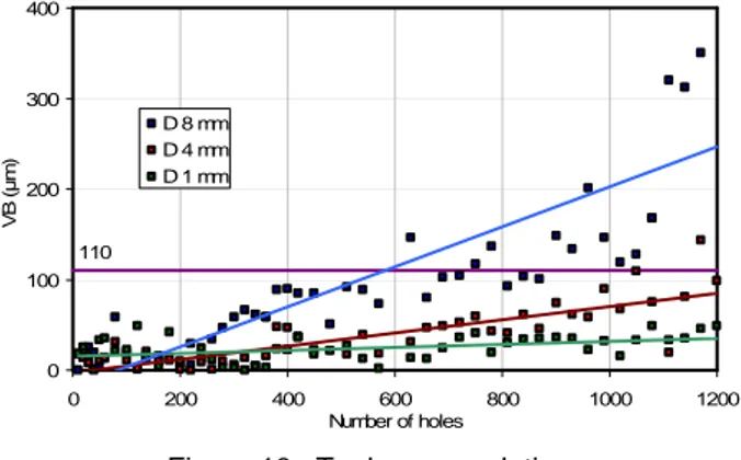
The tool wear is measured very frequently. The criterion chosen to declare the death of the drill is induced by the most penalizing test (higher cutting speed and higher feed). For instance (Figure 18), the value VB = 110 µm has been chosen for the G steel grade.
110 0 100 200 300 400 0 200 400 600 800 1000 1200 Number of holes V B ( µ m ) l D 8 mm D 4 mm D 1 mm
Figure 18: Tool wear evolution G - Vc = 85 m/min - f = 0.11 mm/rev - dry The tool life is expressed as a length, the sum of the depth of the holes being drilled until the tool wear criterion is reached. These tool life values are computed to get the coefficients of the tool life model.
C'' p1 p2
G 1.96 -0.79 -1.97
N 9.33 -2.53 -1.13
Table 5 : Taylor coefficients (tool life criterion VB = 110 µm)
0 .1 1 0 .1 5 0 .1 9 0 .2 3 85 95 105 115 125 0.0 0.5 1.0 1.5 2.0 L (m) f (mm/rev) Vc (m/min)
Figure 19: Drilled length versus Vc and f N - dry
The super high strength of the N steel grade has a very negative effect on the tool life. It appears that the tool life may be up to eight times lower for N than for G steel grade. 0 .1 1 0 .1 5 0 .1 9 0 .2 3 85 95 105 115 125 0 2 4 6 8 10 12 14 16 18 L (m) f (mm/rev) Vc (m/min)
Figure 20: Drilled length versus Vc and f G - dry
The influence of the cutting speed on the tool life is pretty small for the G steel grade. On the N steel grade, the influence of both the cutting speed and feed seems to be equivalent on the operating range drawn here.
These two graphs highlight the same reality for the two steel grades when comparing the following ratio: higher tool life over lower tool life within the cutting range investigated.
For the G steel grade, this ratio is 6.8 (=16.1/2.4) and for the N steel grade it is 6.7 (1.8/0.3). This means that on the operating range of each steel grade, cost estimation will follow the same laws [14].
The time required to drill a hole at Vc = 85 m/min and f = 0.11 mm /rev is 3.3 times higher than at Vc = 125 m/min and f = 0.25 mm/rev.
Thus, the choice of the cutting conditions needs to be done by considering the productivity, the drill costs and the number of parts to be manufactured. This is obviously a simple view of the problem, once the machine, the tool and the material have already been determined.
7 INFLUENCE OF LUBRICATION
The Couple Tool Material approach generally requires to be considered without lubricant. Indeed, this is the best method to be sure the machining operations are done within the exact same conditions of lubrication! Moreover, this makes it possible to take the lubrication issues aside. D 4 mm D 7.5 & 8 mm
D 2 mm D 1 mm
Therefore, the comparison of steel grades machinability or the comparison of tools can be properly done without lubricant.
The purpose is also to show the ability for these materials to be drilled without lubricant, and then to encourage eco-friendly production. However, since the N steel grade appears to be very hard to drill without lubricant, the attempt to drill with lubricant was made.
The tool life is clearly improved when adding the lubricant (Oil SITALA, 6%) (Figure 21). The lubricant has a large impact on the tool life when the feed varies. Indeed, the tool-life in function with the feed has the same behaviour than without lubricant, but the tool life decreases very quickly when increasing cutting speed. When the cutting speed is high, the tool life is the same whether machining is performed dry or not. At low cutting speeds, the tool life is doubled when machining with lubricant. The lubricant seems to be inefficient at high cutting conditions. An internal lubrication could have been more efficient.
0 .1 1 0 .1 3 0 .1 5 0 .1 7 0 .1 9 0 .2 1 0 .2 3 0 .2 5 85 95 105 115 125 0 1 2 3 4 L (m) f (mm/rev) Vc (m/min)
Figure 21: Drilled length versus Vc and f N with external lubricant
These observations are quite interesting. They mean that using lubricant is no necessary if the productivity is preferred to tool life when choosing the cutting conditions. They also mean that lubricant multiplies by two the tool life when machining with low cutting conditions.
8 DISCUSSION - CONCLUSIONS
This paper proposes an application of the Couple Tool Material approach to coated drilling operations. Cutting forces and tool wear are measured and enable to propose relevant operating range. Chip morphology and surface quality analysis confirm the previous results.
To note that the behaviour in the tool-life is hardly dependant of the material machined. The influence of the cutting speed and the feed are induced by the work piece material. This explains the complexity of the extrapolation of the choice of cutting conditions to a new material. The effect of the lubrication on the tool wear has basically been estimated. It is substantial: In the present study, the lubrication increases the tool-life with a ratio up to two.
This factor is also found in the temperature
measurements that are meanly divided by two [15] when machining with lubricant.
The protocol enables to rank the two steel grades developed by ArcelorMittal Gandrange R&D. Collected data are immediately available for ArcelorMittal customers.
9 UNITS
Designation
Unit
Name
Vc m/min Cutting speed
Vz m/s Feed rate
ωz rad/s Rotating speed
f mm/rev Feed per revolution
l mm Hole depth
Ddrill mm Drill diameter
L mm Tool life (a drilled length)
Fz N Measured drilling thrust
Mz N.cm Measured drilling torque
kcMz
kcFz
N/mm2 Specific cutting pressure kcMz ref
kcFz ref
N/mm² Specific cutting pressure model coefficient mcMz ref
mcFz ref
Specific cutting pressure model coefficient
u J/mm3 Specific drilling energy
Pc W Drilling power
T min Tool life
n1, n2, n3, p1, p2 C, C', C''
Tool life model coefficients
10 ACKNOWLEDGMENTS
The experiments have been carried out in the workshop of ENSAM in Metz with the support of Mittal Steel Europe R & D. The authors would like to thank Daniel Boehm, Lionel Simon, Jeremy Bianchin, Frederic Gornay and Didier Cavasino for their involvement in this study.
11 REFERENCES
[1] Bomont, A et Al., 2006, Product-process integration in turning and drilling for forging steels with improved machinability, 5th International Conference on High Speed Machining, Metz, 2006, pp. 39-50.
[2] Resiak, B, 2005, Aciers bas carbone bainitiques microalliés au niobium pour pièces à hautes caractéristiques mécaniques, 33ème Congrès de Traitement Thermique et de l’Ingénierie des Surfaces, Reims, pp. 37-48.
[3] Bomont, A. et Al., 2006, Influence of material structure on deep hole drilling machinability of super high strength steel. Application to crankshaft manufacturing. Methodology, results and analysis. 5th International Conference on High Speed Machining, Metz, 2006, pp. 151-164.
[4] Bomont, A., Confente, M., Bomont, O. Schneider, E., Lescalier, C., Gear hobbing test methodology to evaluate steel machinability, 6th International Conference on High Speed Machining, San Sebastian, 2007, pp. 213-218.
[5] Bomont, A., 2007, Super High Strength Steels for
automotive applications. Investigations in
machinability for dry drilling operations, 10th CIRP international workshop on modelling of machining operations, Reggio Calabria, Italy, pp. 349-356.
[6] AFNOR, 2000, Couple outil-matière, NF E 66-520. [7] Elhachimi, M., Torbaty, S., Joyot, P., 1999,
Mechanical modelling of high speed drilling, International Journal of Machine Tools & Manufacture, vol. 39, pp. 553–581.
[8] Tönshoff, H.K., Spintig, W., König, W., Neises, A., 1994, Machining of holes, Development of drilling technology, Annals of the CIRP, vol. 43/2, pp. 551-561.
[9] Abu-Mahfouz, I, 2003, Drilling wear detection and classification using vibration signals and artificial neural network, International Journal of Machine Tools & Manufacture vol. 43, pp.707–720.
[10] Nouari, M., List, G., Girot, F., Coupard, D., 2003, Experimental analysis and optimisation of tool wear in dry machining of aluminium alloys, Wear, vol. 255, pp. 1359–1368.
[11] Ertunc, H.M., Oysu, C., 2004, Drill wear monitoring using cutting force signals, Mechatronics, vol. 14, pp. 533–548.
[12] Lin, T.-R., 2002, Cutting behavior of a TiN-coated carbide drill with curved cutting edges during the high-speed machining of stainless steel, Journal of Materials Processing Technology, vol. 127,pp. 8–16. [13] Cetim, 1980, Perçage, agrandissement et forage,
ISBN 2 85400 021 8.
[14] Mauchand, M., 2007, Proposal for tool based method of product cost estimation during conceptual design, Journal of Engineering Design, special issue on Cost Engineering, Editor Roy R., Taylor and Francis, ISSN, 0954-4828.
[15] Zeilmann, R.P., 2006, Analysis of temperature during drilling of Ti6Al4V with minimal quantity of
lubricant, Journal of Materials Processing