HAL Id: hal-00520258
https://hal.archives-ouvertes.fr/hal-00520258
Preprint submitted on 22 Sep 2010HAL is a multi-disciplinary open access archive for the deposit and dissemination of sci-entific research documents, whether they are pub-lished or not. The documents may come from teaching and research institutions in France or abroad, or from public or private research centers.
L’archive ouverte pluridisciplinaire HAL, est destinée au dépôt et à la diffusion de documents scientifiques de niveau recherche, publiés ou non, émanant des établissements d’enseignement et de recherche français ou étrangers, des laboratoires publics ou privés.
identification of robot dynamics
Maxime Gautier, Alexandre Janot, Pierre-Olivier Vandanjon
To cite this version:
Maxime Gautier, Alexandre Janot, Pierre-Olivier Vandanjon. A new closed-loop output error method for parameter identification of robot dynamics. 2010. �hal-00520258�
This work has been submitted to the IEEE for possible publication. Copyright may be transferred without notice, after which this version may no longer be accessible p 1
(1)
Université de Nantes,
IRCCyN, 1, rue de la Noë - BP 92 101 - 44321 Nantes Cedex 03, France (2)
HAPTION S.A,
Atelier Relais de Soulgé Route de Laval, 53210 Soulgé sur Ouette, France (3)
Laboratoire Central des Ponts et Chaussées, Route de Bouaye BP 4129, 44341Bouguenais Cedex, France
Abstract—Off-line robot dynamic identification methods are mostly based on the use of the inverse dynamic model, which is linear with respect to the dynamic parameters. This model is sampled while the robot is tracking reference trajectories that excite the system dynamics. This allows using linear least-squares techniques to estimate the parameters. The efficiency of this method has been proved through the experimental identification of many prototypes and industrial robots. However, this method requires the joint force/torque and position measurements and the estimate of the joint velocity and acceleration, through the bandpass filtering of the joint position at high sampling rates. The proposed new method requires only the joint force/torque measurement. It is a closed-loop output error method where the usual joint position output is replaced by the joint force/torque. It is based on a closed-loop simulation of the robot using the direct dynamic model, the same structure of the control law, and the same reference trajectory for both the actual and the simulated robot. The optimal parameters minimize the 2-norm of the error between the actual force/torque and the simulated force/torque. This is a non-linear least-squares problem which is dramatically simplified using the inverse dynamic model to obtain an analytical expression of the simulated force/torque, linear in the parameters. A validation experiment on a 2 degree-of-freedom direct drive robot shows that the new method is efficient.
Keywords — Identification, closed-loop output error, least-squares methods, , robot dynamics.
I. INTRODUCTION
HE usual identification method based on the inverse dynamic identification model (IDIM) and least-squares (LS) technique has been successfully applied to identify inertial and friction parameters of several robotic prototypes and industrial robots [1], [2], [3], [4], [5], [6], [7], [8], [9], [10], [11], [12], [13], [14], [15], amongst others. Good results can be obtained provided a well-tuned derivative bandpass filtering of joint position to calculate the joint velocities and accelerations is used.
Another approach is to minimize a quadratic error between an actual output and a simulated output of the system, assuming both the actual and simulated systems have the same input. This is known as an output error (OE) identification method [16], [17]. The optimal values of the parameters are calculated using non-linear programming algorithms to solve a non-linear least-squares problem. The output is given by a state-space model output equation, which is typically the joint position for mechanical systems. Difficulties arise from the choice of initial conditions, resulting in multiple, local solutions [18]. The OE method has been used to identify electrical parameters of a synchronous machine, and a
A new closed-loop output error method for parameter identification
of robot dynamics
M. Gautier (1), A. Janot (2) and P-O Vandanjon (3)
This work has been submitted to the IEEE for possible publication. Copyright may be transferred without notice, after which this version may no longer be accessible p 2 comparison with the IDIM-LS method showed very similar results [19].
Both IDIM and OE methods require the joint position and the joint force/torque measurements.
The proposed new identification method needs only the joint force/torque measurements. It is based on a closed-loop simulation using the direct dynamic model while the optimal parameters minimize the 2-norm of the error between the actual force/torque and the simulated force/torque, assuming the same control law and the same reference trajectory. This non-linear least-squares problem is dramatically simplified using the inverse dynamic model to formulate the simulated force/torque as an algebraic function linear in relation to the parameters. This paper describes the new identification method and experimental results obtained using a 2 DOF robot.
A condensed version of this work has been presented in [20]. This paper contains detailed proofs to enlighten the theoretical understanding of the method and gives additional experimental results to show the practical efficiency of the method.
The paper is organized as follows: section II reviews the usual identification technique of the dynamic parameters of the robot. Section III presents the output error method. The new identification method is presented in section IV. The modeling of the SCARA prototype robot is presented in section V. This direct drive prototype is very well suitable for the study of the method because it emphasizes non linear coupling while it is divided by the squared high gear ratio for industrial robots. The experimental results are given in section VI. Finally, section VII is the conclusion.
II. IDIM:INVERSE DYNAMIC IDENTIFICATION MODEL TECHNIQUE
The inverse dynamic model (IDM) of a rigid robot composed of n moving links calculates the motor torque vector τidm, as a function of the generalized coordinates and their derivatives. It can be obtained from the Newton-Euler or the Lagrangian equations [13], [21]. It is given by the following relation:
= ( ) + ( , ) idm
τ M q q&& N q q& (1)
Where q , q& and q&& are respectively the
( )
n 1x vectors of generalized joint positions, velocities and accelerations, M q is the ( )( )
n n robot inertia matrix, and x N q q( , )& is the( )
n 1 vector of centrifugal, x Coriolis, gravitational and friction forces/torques.The choice of the modified Denavit and Hartenberg frames attached to each link allows a dynamic model that is linear in relation to a set of standard dynamic parameters, χ [3], [22]: st
(
)
idm st st
τ =IDM q,q,q χ& && (2)
This work has been submitted to the IEEE for possible publication. Copyright may be transferred without notice, after which this version may no longer be accessible p 3 standard parameters given by:
T T T T ... 1 2 n st st st st χ =χ χ χ with: T j j st XXj XYj XZj YYj YZj ZZj MXj MYj MZj Mj Iaj Fvj Fcj off χ = τ (3) where:
• XX , XY , XZ , YY , YZ , ZZ are the six components of the inertia matrix, j j j j j j jJ , of link j at the j
origin of frame j,
• MX , MY , MZ are the components of the first moments,j j j jMS , of link j, j • M is the mass of link j, j
• Ia is a total inertia moment for rotor and gears of actuator j. j
• Fv , j Fc are the viscous and Coulomb friction parameters of joint j. j •
j
off Fsj tj
τ =Of +Of is an offset parameter where OfFsj is the dissymmetry of the Coulomb friction with respect to the sign of the velocity and Of is due to the current amplifier offset which supplies tj the motor.
• Ns=14* n is the number of standard parameters.
The base parameters are the minimum number of dynamic parameters from which the dynamic model can be calculated. They are obtained from the standard inertial parameters by eliminating those which have no effect on the dynamic model, and by regrouping some others by means of linear relations. They can be determined using simple closed-form rules [22] or a numerical method based on the QR decomposition [23].
The minimal inverse dynamic model can be written as:
(
)
idm
τ =IDM q,q,q χ& && (4)
Where:
(
)
IDM q,q,q& && is the
( )
n b matrix of the minimal set of basis functions of the rigid body dynamics, x (5)χ is the
( )
b 1 vector of the b base parameters. x (6) Because of perturbations due to noise measurement and modeling errors, the actual force/torque τ differs from τidm by an error, e , such that:(
)
idm
τ e IDM q,q,q χ e
τ= + = & && + (7)
Equation (7) represents the Inverse Dynamic Identification Model (IDIM).
We consider the off-line identification of the base dynamic parameters χ , given measured or estimated off-line data for τ and
(
q, q, q & &&)
, collected while the robot is tracking some plannedThis work has been submitted to the IEEE for possible publication. Copyright may be transferred without notice, after which this version may no longer be accessible p 4 trajectories.
Usually, the signals available from the robot controller are the joint position measurement and the
( )
n 1 control signal vector vx τ, calculated according to the control law.Then
(
q, q, q & &&)
in (7) are estimated with(
ˆq, q, q & &&ˆ ˆ)
, respectively, obtained by bandpass filtering the measure of q [9]. The derivatives are calculated off-line without phase shift, using a central difference algorithm of the lowpass filtered position ˆq . The filtered position ˆq is calculated off-line with a non causal zero-phase digital filter by processing the input data, q , through a lowpass Butterworth filter in both the forward and reverse direction using the filtfilt procedure from Matlab.The control signal, vτ, is connected to the input current reference of the current closed-loop of the amplifiers which supplies the motors. Assuming that the current closed-loop has a bandwidth greater than 500Hz, then its transfer function is equal to its static gain, K , in the frequency range (less than c
10Hz) of the rigid robot dynamics. Then, the actual force/torque, τ, is calculated with the relation:
g vτ τ
τ= (8)
where:
gτ, is the
( )
nxn diagonal matrix of the drive gains, with:r c
gτ =K K Kτ (9)
where: r
K , is the
( )
nxn gear ratios diagonal matrix of the joint drive chains (&qm=K qr& , with &qm, the velocity on the motor side),c
K , is the
( )
nxn static gains diagonal matrix of the current amplifiers,Kτ, is the
( )
nxn diagonal matrix of the electromagnetic motor torque constants.Those parameters have a priori values, given by manufacturers, which can be checked with special tests [24].
The inverse dynamic identification model (IDIM) (7) is calculated at a frequency measurement f , m using samples of
(
ˆq, q, q & &&ˆ ˆ)
to calculate IDM q,q,q(
ˆ & &&ˆ ˆ)
and samples of vτ to calculate τ with (8), at different times tk, k =1,...,nm, while the robot is tracking a reference trajectory(
q ,q ,qr & &&r r)
, during the time length Tobs, of the trajectory.This work has been submitted to the IEEE for possible publication. Copyright may be transferred without notice, after which this version may no longer be accessible p 5
The equations of each joint are regrouped together on all the trajectory to get an over-determined linear system such that:
( )
( )
fm fm ˆ ˆ ˆ fm Y τ =W q,q,q χ& && +ρ (10) With:( )
m 1 fm j 1 j fm fm n fm j n Y ( t ) Y τ ... , Y ... Y ( t ) τ τ = = (11)(
)
( ( ) ( ) ( )) ( ( ) ( ) ( ) m m m 1 j fm 1 1 1 j fm fm n j fm n n n ˆ ˆ ˆ W IDM q t ,q t ,q t ˆ ˆ ˆ W q,q,q ... , W ... ˆ ˆ W IDM q tˆ ,q t ,q t = = & && & && & && (12) where: ( ( ) ( ) ( )) j k ˆ k ˆ k ˆIDM q t ,q t ,q t& && is the jth row of the
( )
n b matrix of the basis functions, x ( ( ) ( ) ( ))ˆ k ˆ k ˆ kIDM q t ,q t ,q t& && , (5), j
fm
Y and Wfmj represent the nmequations of joint j , *
m obs m
n =T f is the number of sample measurements.
The notation Wfm
(
IDM q,q,q(
ˆ & &&ˆ ˆ)
)
=Wfm( )
q,q,qˆ & &&ˆ ˆ , will be used to recall that W , is calculated with a fm sampling of IDM q,q,q(
ˆ & &&ˆ ˆ)
.In order to eliminate high frequency force/torque ripple in τ , and to window the identification frequency range into the model dynamics, a parallel decimation procedure lowpass filters in parallel Y fm and each column of W and resamples them at a lower rate, keeping one sample over fm n . This parallel d
decimation can be carried out with the Matlab decimate function, where the lowpass filter cut-off
frequency is equal to 0.8* /(2*fm nd).
After the data acquisition procedure and the parallel decimation of (10), we obtain the over-determined linear system:
( )
( )
ˆ ˆ ˆY τ =W q,q,q χ& && +ρ (13)
where:
• Y τ is the
( )
( rx1) vector of measurements, built from the actual force/torque τ ,This work has been submitted to the IEEE for possible publication. Copyright may be transferred without notice, after which this version may no longer be accessible p 6
• ρ is the ( rx1) vector of errors.
• r=n* n / nm d is the number of rows in (13).
In Y and W , the equations of each joint are grouped together such that:
, 1 1 n n Y W Y ... W ... Y W = = (14)
where Y and j W represent the j n / n equations of joint j . m d
The ordinary LS (OLS) solution ˆχ minimizes the squared 2-norm ρ 2 of the vector of errors.
Using the base parameters and tracking “exciting” reference trajectories [25], we get a full rank and well conditioned matrix W . The LS solution ˆχ is given by:
(
)
(
T 1 T)
ˆχ= W W − W Y =W Y+ (15)
It is computed using the QR factorization of W . Standard deviations
i
ˆ χ
σ , are estimated using classical results from statistics under the assumptions that W is a deterministic matrix, according to the data filtering procedure described above, and ρ , is a zero-mean additive independent Gaussian noise, with a covariance matrix Cρρ, such that:
T 2
ρρ ( ) σρ r
C =E ρρ = I (16)
where E is the expectation operator and Ir, the
( )
r rx identity matrix.An unbiased estimation of the standard deviation σρ is:
2 2
ρ
σˆ = Y−Wχˆ (r−b ) (17)
The covariance matrix of the estimation error is given by:
T 2 T 1 χχ [( )( ) ] σρ( ) ˆ ˆ ˆ ˆ ˆ C =E χ−χ χ−χ = W W − (18) i 2 χ χχ σˆ =C (ˆ ˆ i ,i) is the i th diagonal coefficient of χχ ˆ ˆ
C . The relative standard deviation
ri χ %σˆ is given by: ri i χ χ i %σˆ =100σˆ χˆ , for ˆ ≠ 0 χi (19)
The OLS can be improved by taking into account different standard deviations on joint j equations errors [9]. Each equation of joint j in (13), (14), is weighted with the inverse of the standard deviation of the error calculated from OLS solution of the equations of joint j , given by:
( )
(
(
)
)
j j j j
j ˆ ˆ ˆ
This work has been submitted to the IEEE for possible publication. Copyright may be transferred without notice, after which this version may no longer be accessible p 7
This weighting operation normalises the errors in (13) and gives the weighted LS (WLS) estimation of the parameters.
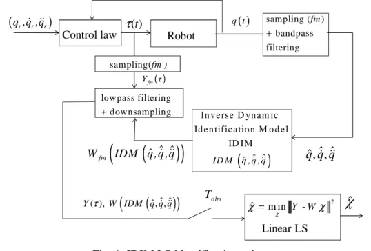
This identification method is illustrated in Fig. 1.
Compared with the OE method described in the following section III, the use of IDIM, which is an analytical function of
(
q,q,q& &&)
, is particularly interesting because it does not require the integration of the direct dynamic model (21). Moreover, ˆχ is a one step linear LS solution which does not need initialconditions. However, the calculation of the velocities and accelerations are required using well-tuned bandpass filtering of the joint position [9].
Robot
(
)
In v e rse D yn a m ic Id e n tific a tio n M o d e l ID IM ˆ ˆ ˆID M q , q , q& && q q qˆ, ,ˆ ˆ& &&
(
)
(
)
fm ˆ ˆ ˆ
W IDM q ,q ,q& &&
Linear LS 2 ˆ m in Y -W χ χ = χ
(
)
(
ˆ ˆ ˆ)
( ), , ,Y τ W IDM q q q& &&
( ) q t ( )t τ Control law
ˆ
χ
(
q ,q ,qr & &&r r)
obs T sampling ( ) bandpass filtering fm + lowpass filtering + downsampling sampling(fm ) ( ) fm Y τFig. 1. IDIM LS identification scheme. III. THE OUTPUT ERROR METHOD (OE)
The OE identification methods minimize a quadratic error between an actual output y , and a simulated output y , of the system, assuming both the actual and the simulated systems have the same s
input. This approach can be implemented in an open-loop form, [17], [26], or in a closed-loop form, [27], [28]. Considering a closed-loop controlled robot, the input, in the open loop scheme shown in Fig. 2, is the actual force/torque τ , and the input, in the closed-loop scheme shown in Fig. 3, is the reference trajectory
(
q ,q ,qr & &&r r)
. Because the open loop simulation of unstable robotic systems is very sensitive to the initial state conditions and to the errors in numerical algorithms which solve the differential equations, it is more suitable to choose the closed-loop form.This work has been submitted to the IEEE for possible publication. Copyright may be transferred without notice, after which this version may no longer be accessible p 8 taking the measured joint position as the output, the actual output is, y=q, and the simulated output is,
s ddm
y =q , as shown in Fig. 2 and Fig. 3, where qddm( t ) , is the solution of the differential equation given by the Direct Dynamic Model (DDM).
The DDM can be obtained by writing the IDM equation (1), as following: ( ddm, ) ddm = ddm - ( ddm, ddm, )
M q χ &&q τ N q &q χ (21)
where: ( ddm, )
M q χ and N q( ddm, &qddm, )χ depend on an estimation of the base parameters χ, ddm
τ , is the force/torque input of the DDM.
The function qddm
( )
t ,χ , is the result of the integration of the linear implicit differential equation (21) which can be written as a non-linear state-space model:s s s s G( x )x& = f ( x ,u ) (22) where: ddm s ddm q x q =
& , is the
(
2* nx1)
state-space vector, s ddmu =τ , is the ( x1)n control input,
x x G ( , ) - ( , , ) n n n ddm s s s n n ddm ddm ddm ddm I 0 q ( x ) , f ( x ,u ) 0 M q χ τ N q q χ = = & & (23)
where, 0n nx , is a ( x )n n , matrix of zeros.
The linear output equation is given by:
s s s s s
y =C x +D u (24)
Taking the measure of joint position as the output, ys =qddm, we get:
[
x2]
s n n *n
C = I 0 , is the, ( x2* )n n , output matrix, (25)
x
s n n
D =0 , is the, ( x )n n , direct feedthrough matrix. (26)
Hence, for robotic systems, an OE identification method is based on the integration of the Direct Dynamic Model.
The optimal solution ˆχ, minimizes the quadratic criterion J
( )
χ , given by:( )
2(
) (
T)
s s s
J χ = Y −Y = Y −Y Y −Y (27)
This work has been submitted to the IEEE for possible publication. Copyright may be transferred without notice, after which this version may no longer be accessible p 9
Y and Y , are vectors obtained by filtering the vectors of samples s Y and fm YSfm, respectively, where the equations of each joint are grouped together, with:
m 1 fm j 1 j fm fm n fm j n Y q ( t ) Y ... , Y ... Y q ( t ) = = = , 1 Sfm ddm 1 j Sfm Sfm n Sfm ddm k Y q ( t ) Y ... , Y ... Y q ( t ) = = (28)
The minimization of J
( )
χ , (27), is a non-linear least-squares problem. The estimation of the parameters can be computed using algorithms such as the gradient method, the Newton methods or the Levenberg Marquardt method. These methods are based on a first or second order Taylor’s expansion of( )
J χ .
Actual Robot
Direct Dynamic Model (DDM)
ddm ddm ddm ddm ddm M( q ) q&& =τ − N( q , q& ) Non Linear LS 1 min 2 2 s ˆ Y Y χ χ = − ( )t τ Control law r r r q q q & && ˆ χ Sampling and filtering ( ), (s ddm) Y q Y q
( )
s ddm y =q t obs T ( ) y=q t ( )t τFig. 2. Open-loop OE identification scheme.
Actual Robot
Direct Dynamic Model (DDM)
ddm ddm ddm ddm ddm M( q ) q&& =τ −N( q , q& ) Non Linear LS 1 min 2 2 s ˆ Y Y χ χ = − ( )t τ Control law r r r q q q & && ˆ χ Sampling and filtering ( ), (s ddm) Y q Y q
( )
s ddm y =q t obs T ddm τ ( ) y=q t Control lawThis work has been submitted to the IEEE for possible publication. Copyright may be transferred without notice, after which this version may no longer be accessible p 10
Fig. 3. Closed-loop OE identification scheme.
In [20], we used the Gauss-Newton method to calculate the optimal solution. It is a Newton method where approximations of the gradient and the hessian of J
( )
χ are calculated with the jacobian matrix of y with respect to χ . The Gauss-Newton regression is a simpler way to calculate the optimal solution s[29]. It is based on a Taylor series expansion of y , at a current estimate s k ˆχ , of the parameters at iteration k :
(
)
(
)
+1 +1 k k k S k k S S ˆχ y ( χ ) ˆ ˆ y ( χ ) y ( χ ) χ χ o χ ∂ = + − + ∂ (29) where:(
)
s y / k S χ ˆχ y ( χ ) δ χ ∂ = ∂ (30) s y /χδ is the
( )
n b , jacobian matrix of x y , with respect to χ , evaluated at s kˆχ .
Each coefficient of
s
y /χ
δ , defines a sensitivity function.
These sensitivity functions characterize the variation of the output function y , with respect to a S
variation of the parameter χ . The sensitivity functions are the solutions of a differential system calculated from (21). However, this technique is more time-consuming compared to the IDIM method. Indeed, the DDM and the sensitivity functions must be integrated many times at each step of the iterative non-linear optimization method. Moreover, it is necessary to have good initial conditions in order to avoid multiple and local solutions.
Let us define: +1 y = yS( χk )+ e (31) From (29), it becomes:
(
+1)
(
)
/ s k k k s ˆ y χ ˆ y−y ( χ )=δ χ −χ + +o e (32)An over-determined linear system is obtained by filtering and sampling (32) over the time window Tobs:
+1 k δ Y W χ ∆ = ∆ +ρ (33) with:
(
)
+1 +1 k k ˆk χ χ χ ∆ = −This work has been submitted to the IEEE for possible publication. Copyright may be transferred without notice, after which this version may no longer be accessible p 11
Y
∆ , W , and δ ρ are, respectively, the sampling and filtering of
(
y−y ( χ )s ˆk)
, /s y χ δ , and of
(
o e+)
. +1 k ˆχ∆ is the LS solution of (33). This process is iterated with a new estimate, χˆk+1= χˆk+∆ˆχk+1, until:
k 1 k k 1 tol ρ ρ ρ + − ≤ , and, ik+1 ik 2 k i 1,...,b i ˆχ ˆχ max tol ˆχ = − ≤ (34) where, tol and 1 tol , are values ideally chosen to be small numbers to get fast convergence with good 2 accuracy.
IV. DIDIM:DIRECT AND INVERSE DYNAMIC IDENTIFICATION MODEL TECHNIQUE
A. Theoretical approach
In the OE method as shown in Fig. 3, the actual output is the measured joint position, y=q.
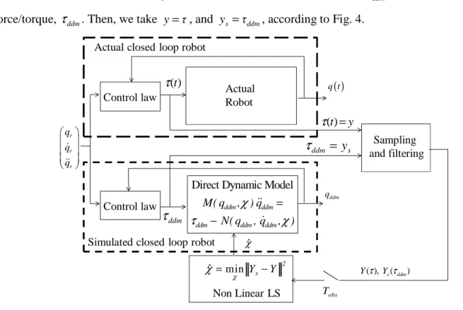
We propose to change the output, y , from the actual joint position q , to the actual joint force/torque τ, and the simulated output ys, from the simulated joint position, qddm, to the simulated joint force/torque, τddm. Then, we take y=τ, and ys=τddm, according to Fig. 4.
Actual Robot
Direct Dynamic Model ddm ddm ddm ddm ddm M( q , ) q N( q , q , ) χ τ χ = − && & Non Linear LS min s 2 ˆ Y Y χ χ = − ( )t τ Control law r r r q q q & && ˆ χ Sampling and filtering ( ), (s ddm) Yτ Y τ obs T ddm
τ
( ) q t Control law ddm ysτ
= ( )t y τ = ddm qActual closed loop robot
Simulated closed loop robot
Fig. 4. DIDIM identification scheme.
This means that the output equation (24) of the state-space model (22) reduces to a direct feedthrough equation such as, ys = =us τddm.
This work has been submitted to the IEEE for possible publication. Copyright may be transferred without notice, after which this version may no longer be accessible p 12
The optimal solution, ˆχ, minimizes the quadratic criterion, J
( )
χ , (27), where, Y , and Ys, are vectors obtained by filtering the vectors of samples, Yfm and YSfm, respectively, where the equations of each joint are grouped, with:( )
m 1 fm j 1 j fm fm n fm j n Y ( t ) Y τ ... , Y ... Y ( t ) τ τ = = , j j m 1 ddm 1 Sfm j Sfm Sfm n Sfm ddm n ( t ) Y Y ... , Y ... Y ( t ) τ τ = = (35)This non-linear LS problem is solved by the Gauss-Newton regression as explained in section III. The input force/torque of the DDM, τddm, can be calculated with the analytical expression of the inverse dynamic model (4), such as:
( )
( )
( )
(
( )
( )
( )
)
s ddm idm ddm ddm ddm
y χ =τ χ =τ χ =IDM q χ ,q& χ ,q&& χ χ (36) The Taylor series expansion (29), with ys =τddm, at a current estimate, ˆχ , of the parameters χ , at k
iteration k , is calculated with the jacobian matrix of τddm
( )
χ , given by:( )
( )
(
(
)
)
s y / k k k k k k ddm idm χ ddm ddm ddm ˆ ˆ χ χ ˆ ˆ ˆ ˆ δ IDM q ( χ ),q ( χ ),q ( χ ) χ χ χ χ τ τ ∂ ∂ ∂ = = = ∂ ∂ ∂ & && (37) Then, it becomes:(
)
(
)
(
)
(
)
(
)
k k k k k k k ddm ddm ddm ddm ddm ddm k k k k ddm ddm ddm ˆ ˆ ˆ ˆ ˆ ˆ ˆ IDM q ( χ ),q ( χ ),q ( χ ) χ IDM q ( χ ),q ( χ ),q ( χ ) ... χ ˆ ˆ ˆ ˆ IDM q ( χ ),q ( χ ),q ( χ ) χ χ ∂ = + ∂ ∂ ∂& && & &&
& &&
(38)
The calculation of the second term on the right side of (38) needs to calculate the expression:
(
)
(
)
(
(
)
)
(
)
(
)
(
)
(
)
k k k k k k ddm ddm ddm ddm ddm ddm ddm ddm k k k ddm ddm ddm ddm ddm k k k ddm ddm ddm ddm ddm q ˆ ˆ ˆ ˆ ˆ ˆ IDM q ( χ ),q ( χ ),q ( χ ) IDM q ( χ ),q ( χ ),q ( χ ) ... χ q χ q ˆ ˆ ˆ IDM q ( χ ),q ( χ ),q ( χ ) ... q χ q ˆ ˆ ˆ IDM q ( χ ),q ( χ ),q ( χ ) q χ ∂ = ∂ ∂ + ∂ ∂ ∂ ∂ ∂ + ∂ ∂ ∂ ∂ ∂ ∂& && & &&
& & && & && & && && (39)
Let us recall that the joint force/torque y=τ, is obtained while the robot is tracking a reference trajectory,
(
q ,q ,qr & &&r r)
, with a closed-loop control law. The closed-loop simulation uses the direct dynamic model, the same control law and the same reference trajectory(
q ,q ,qr & &&r r)
, as the actual one, to calculate yS.This work has been submitted to the IEEE for possible publication. Copyright may be transferred without notice, after which this version may no longer be accessible p 13 order to keep the same bandwidth and stability margin as the actual closed-loop for any ˆχ , obtained at k
iteration k. This assumes for the simulated tracking error to keep close to the actual one for any ˆχ , that k
is to say:
(
k k k)
(
)
ddm ˆ ddm ˆ ddm ˆ
q ( χ ),q& ( χ ),q&& ( χ ) q,q,q& && , for any ˆχ k (40) This means that
(
qddm( χ ),q&ddm( χ ),q&&ddm( χ ))
, have little dependence on χ , such that:ddm ddm ddm q q q 0 χ χ χ ∂ ∂ ∂ ∂ &∂ &&∂ Then (39) is simplified as:
(
)
(
IDM qddm( χ ),qˆk ddm( χ ),qˆk ddm( χ )ˆk)
0χ
∂
∂ & &&
Taking into account this simplification, we have in (38):
(
)
(
k k k)
(
k k k)
ddm ˆ ddm ˆ ddm ˆ ˆk ddm ˆ ddm ˆ ddm ˆ IDM q ( χ ),q ( χ ),q ( χ ) χ IDM q ( χ ),q ( χ ),q ( χ ) χ ∂∂ & && & &&
As a result, the jacobian matrix (37) can be approximated by:
(
)
(
)
(
)
s y / k k k k k k k χ ddm ˆ ddm ˆ ddm ˆ ˆ ddm ˆ ddm ˆ ddm ˆ δ IDM q ( χ ),q ( χ ),q ( χ ) χ IDM q ( χ ),q ( χ ),q ( χ ) χ ∂ =∂ & && & && (41)
Each sensitivity function in the jacobian matrix is approximated by an algebraic equation. This is much more simpler than for usual OE method where the sensitivity functions are the solutions of complicated differential equations. This is the reason why it is much more simpler to minimize the error between the measured force/torque and the simulated force/torque than to minimize the error between the actual position and the simulated position.
Taking the approximation (41) of the jacobian matrix into the Taylor series expansion (32), it becomes:
(
)(
+1)
(
)
k k k k k k
s ˆ ddm ˆ ddm ˆ ddm ˆ ˆ
y= =τ y ( χ )+IDM q ( χ ),q& ( χ ),q&& ( χ ) χ −χ + +o e (42) From (36), it becomes:
(
)
k k k k k k
s ˆ idm ˆ ddm ˆ ddm ˆ ddm ˆ ˆ
y ( χ )=τ ( χ )=IDM q ( χ ),q& ( χ ),q&& ( χ ) χ (43) Taking (43) in (42), it becomes:
(
k k k)
k+1(
)
ddm ˆ ddm ˆ ddm ˆ
y= =τ IDM q ( χ ),q& ( χ ),q&& ( χ ) χ + +o e (44) This is the Inverse Dynamic Identification Model, IDIM, (7), where
(
q, q, q & &&)
are estimated with(
qddm,q&ddm,q&&ddm)
, simulated withk
ˆ
This work has been submitted to the IEEE for possible publication. Copyright may be transferred without notice, after which this version may no longer be accessible p 14 described in section II.
The sampling of (44) at a sampling rate f , gives an over-determined linear system such as: m
( )
(
, k)
fm fm ddm ddm ddm ˆ fm Y τ =Wδ q ,q& ,q&& χ χ+ρ (45) With:( )
m 1 fm j 1 j fm fm n fm j n Y ( t ) Y τ ... , Y ... Y ( t ) τ τ = = (46)(
)
(
( )
( )
( )
)
( )
( )
( )
(
)
1 1 1 , , , m m m j k 1 ddm ddm ddm fm k j fm ddm ddm ddm fm n j k fm ddm n ddm n ddm n ˆ IDM q t ,q t ,q t χ W ˆ W q ,q ,q χ ... , W ... W IDM q t ,q t ,q t ˆχ δ δ δ δ = = & && & && & && (47)The parallel decimation of (45) gives:
( )
(
ddm ddm ddm,ˆk)
Y τ =W qδ ,q& ,q&& χ χ+ρ (48)
The LS solution of (48) gives ˆχk 1+ , at iteration +k 1. This process is iterated until:
k 1 k k tol1 ρ ρ ρ + − ≤ , and, ik+1 ik 2 k i 1,...,b i ˆχ ˆχ max tol ˆχ = − ≤ ,
where, tol and 1 tol are values ideally chosen to be small numbers to get fast convergence with good 2 accuracy.
This new identification method is based on a closed-loop simulation using the direct dynamic model (DDM) while the optimal parameters minimize the 2-norm of the error between the actual force/torque τ, and the simulated force/torque τddm, over an observation window time Tobs. This new technique overcomes the problems of non-linear optimization in OE method, section III, using the IDIM to calculate the simulated force/torque vector, ys =τddm =τidm. Because this method uses both models DDM and IDIM, it is named the DIDIM method: Direct and Inverse Dynamic Identification Models technique.
The DIDIM method with the Gauss-Newton regression is illustrated Fig. 5. This approach is particularly interesting thanks to the following reasons: • It needs only the actuator force/torque measurement or estimation,
• It avoids tuning the bandpass filter in the IDIM method by using the integration of the DDM in a closed-loop simulation where the tuning of the bandwidth automatically defines the same frequency
This work has been submitted to the IEEE for possible publication. Copyright may be transferred without notice, after which this version may no longer be accessible p 15
range for the dynamics of the actual and of the model to be identified.
• It combines the inverse and the direct dynamic model and validates, in the same identification procedure, both models for computed torque control and for simulation.
• It dramatically simplifies the computation of the matrix of the sensitivity functions which is given by an algebraic equation (the inverse dynamic identification model) whereas it is given by the resolution of a complicated system of differential equations in the usual OE method.
The drawback is that the structure and the tuning of the actual closed-loop control law must be known to be implemented in the closed-loop simulation of the robot. Most often, this is not a real problem, because working on identification for simulation or control of the robot, needs a minimal knowledge on the robot controller.
r r r q q q & && Actual Robot
Direct Dynamic Model
k ddm ddm k ddm ddm ddm ˆ M( q , ) q ˆ N( q , q , ) χ τ χ = − && & Linear LS +1 min 2 k ˆ Y Wδ χ χ = − χ ( )t τ Control law ˆ χ ( )
(
ˆ)
( ), W , , , k ddm ddm ddmYτ δ IDM q q& q&& χ
obs T ddm τ ( ) q t Control law
(
)
Inv erse D ynam ic Id entificatio n M o d el k d dm dd m dd m ˆ ID M q ,q& ,q&& ,χ
(
k)
ddm ddm ddm ˆIDM q ,q& ,q&& ,χ
( )t y
τ =
ddm
q
Actual closed loop robot
Simulated closed loop robot
sampling ( ) lowpass filtering downsampling
fm
Fig. 5. DIDIM with the Gauss-Newton regression, identification scheme.
B. Initialization of the algorithm
A problem is how to choose the initial values 0
ˆχ .
We can use CAD values, or identified values with the IDIM method, but we show that there is no need at all of a priori values.
We propose an algorithm not sensitive to the initial conditions, which assumes that the condition
(
qddm( χ ),qˆk &ddm( χ ),qˆk &&ddm( χ )ˆk) (
q,q,q& &&)
, is satisfied at any iteration k , and especially for k =0.This is possible by taking the same control law structure for the actual robot and for the simulated one with the same performances given by the bandwidth, the stability margin or the closed-loop poles.
This work has been submitted to the IEEE for possible publication. Copyright may be transferred without notice, after which this version may no longer be accessible p 16 Because the simulated robot parameters ˆχ , change at each iteration k , the gains of the simulated k
control law must be updated according to ˆχ . k
For example, let us consider a PD control law for each joint j . The inverse dynamic model IDM (1) for the joint j , can be written as a decoupled double integrator perturbed by a coupling force/torque, such that: = ( ) + ( , )= ( ) ( ) + ( , )= ( ) j n n j idm j ,i i j j , j j j ,i i j j , j j j i 1 i j τ τ M q q N q q M q q M q q N q q M q q p = ≠
=
∑
&& & && +∑
&& & && − (49)where p is considered as a perturbation given by: j
( ) ( , ) n j j ,i i j i j p M q q N q q ≠ = −
∑
&& − & (50) ( ) j ,iM q which depends on q , is approximated by a constant inertia moment J , given by: j
(
( ))
j j j j a j , j j a q J =ZZ +I +max M q −ZZ −I (51) jJ , is the maximum value, with respect to q , of the inertia moment around joint zj axis. This gives the smallest damping value and the smallest stability margin of the closed-loop second order transfer function (55), while q varies.
It can be calculated from a priori CAD values of inertial parameters and must be taken at least as
j
j a
ZZ +I .
The joint j dynamic model is approximated by a double integrator, where p , is a perturbation, as j
following:
(
)
(
)
( ) j j j j j j , j j 1 1 q τ p τ p M q J = + + && (52)Let us consider the joint j PD control of the actual robot which is illustrated Fig. 6:
+ - +- j a gτ j r q j a v k a1 j J 1 s 1 s ++ j a p k j p j vτ τj q&&j q&j qj
Fig. 6. Joint PD control of the actual robot. The control input calculated by the robot controller is given by:
This work has been submitted to the IEEE for possible publication. Copyright may be transferred without notice, after which this version may no longer be accessible p 17
(
)
j j j j j a a a p v r j v j vτ = k k q −q − k q& (53) jvτ is the current reference of the current amplifiers which supplies the motor. The joint j , force/torque is given by:
j j a j g vτ τ τ = (54) where: j a
gτ is the actual drive gain, calculated with the actual parameters in (9). a
j
J is the actual value of Jj.
In order to tune the tracking performances of the reference position
j
r
q , the transfer function rj
j q q is calculated with pj=0: =0 j j j j j j j j a 2 2 a j j r p a a a a a 2 a v p p nj nj q 1 1 H J s 2 q 1 s s 1 s 1 gτ k k k ζ ω ω = = = + + + + (55) where: a nj
ω is the actual natural frequency which characterizes the closed-loop bandwidth, a
j
ζ is the actual damping coefficient which characterizes the closed-loop stability margin, with:
j i i a a a a nj p v a j g k k J τ ω = , 1 i j i a a v a j a a p j g k 2 k J τ ζ = (56) Then it becomes: 2 j a nj a p a j k ω ζ = , j j a j a a a v j nj a J k 2 gτ ζ ω = (57)
The closed-loop performances are chosen with the desired 2 poles of a second order transfer function characterized by, dωnj, dζj, where:
d nj
ω is the desired natural frequency, d
j
ζ is the desired damping coefficient.
Because the actual values are unknown, the gains are calculated from (57), where the unknown actual values, aωnj, aζj, aJj,
j
a i
g , are replaced respectively by their desired values, dωnj, dζj, and by their a priori values, apJ ,j
j
ap
This work has been submitted to the IEEE for possible publication. Copyright may be transferred without notice, after which this version may no longer be accessible p 18
2 j d nj a p d j k ω ζ = , j j ap j a d d v j nj ap J k 2 gτ ζ ω = (58) where: and j ap ap j
J gτ are a priori values of the actual unknown values and
j
a a
j
J gτ , respectively.
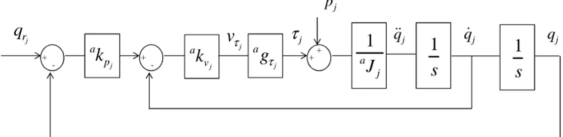
Now, let us consider the joint j PD control of the simulated robot which is illustrated Fig. 7.
+ - +- j ap gτ j r q j s v k 1k j ˆJ 1 s 1 s ++ j s p k j ddm p j ddm vτ j ddm q& qddmj j ddm τ q&&ddmj
Fig. 7. Joint PD control of the simulated robot.
The variables
(
,)
j j j j j
ddm ddm ddm ddm ddm
vτ ,τ q , q& , q&& , in Fig. 7, are computed by numerical integration of k
ˆ
DDM ( χ ) , (21).
The control law of the simulated robot has the same structure as the actual one, Fig. 6, where we take:
j a i g = j ap i
g , the a priori value of j a i g , a j
J =ˆJ , the value of kj J , (51), calculated with the estimation j χˆk, at iteration k.
j s p k , j s v
k are the gains of the simulated control law.
They are calculated in order to keep the same performances for the simulated closed-loop and for the actual closed-loop, that is to say to keep the same desired values, dωnj and dζj, for the closed-loop poles. Then, it becomes:
, 2 2 j j j j d k nj j s a s d d p d p v j nj ap j ˆJ k k k gτ ω ζ ω ζ = = = (59)
The proportional gain,
j
s p
k , does not depend at all on the parameters values, but the derivative gain in
the simulator ,
j
s v
k , must be updated with ˆJ , at each iteration k . kj
It is important to note that only the gain in the simulated closed-loop,
j
s v
k , is modified during the
iterative procedure. The actual gain of the robot control law,
j
a v
k , is not modified.
This work has been submitted to the IEEE for possible publication. Copyright may be transferred without notice, after which this version may no longer be accessible p 19 following ratio, calculated by taking (58) into (56):
j j a a a ap nj j j d d a ap nj j j g J J g τ τ ω ζ ω = ζ = (60)
Usually this ratio is between 0.8 and 1.2. The actual values, aωnj, aζj, can be estimated from step response or frequency analysis of the actual closed-loop. But this is not necessary, because there is little effect on the identification accuracy, assuming, dωnj, is regularly chosen more than 10 times greater than the frequency range of the robot dynamics.
This allows to keep
(
qddm( χ ),qˆk &ddm( χ ),qˆk &&ddm( χ )ˆk) (
q,q,q& &&)
, at each iteration k.We propose to take a regular inertia matrix M q( ddm,χˆ0) , in order to have a good initialization for the numerical integration of the DDM (21) . This is named the "regular initialization".
It can be obtained with:
0
0
ˆ
χ = , except for, Ia0j =1, j=1,n (61)
The inertia of the rotor and gear of actuator j is generally taken into account in the IDM model (1) as: τ
j
r Ia q= j&&j
Then, the initial inertia matrix becomes the identity matrix, which is the best regular matrix:
0
( ddm,ˆ ) = n
M q χ I (62)
Another simple regular initialization is to take:
0
0
ˆ
χ = , except for, ZZ0j =1, j=1,n (63)
The initial inertia matrix, M q( ddm,χˆ0), is no more the identity matrix, but remains regular.
Another point is to choose the state initial condition of the state vector,
(
qddm(0),q&ddm(0))
, in order to integrate the DDM (21). Because DIDIM doesn't need the joint position measurement, the actual values(
q(0) (0),q&)
, are supposed to be unknown and we choose,(
qddm(0),q&ddm(0)) (
= qr(0),q&r(0))
, which is close to(
q(0) (0),q&)
. Because the closed-loop transient response due to different initial conditions differs between the actual and the simulated signals during a transient period of approximately, 5/ dωn, the corresponding joint force/torque samples are eliminated from the identification data in (45).V. CASE STUDY: MODELING OF THE SCARA ROBOT
This work has been submitted to the IEEE for possible publication. Copyright may be transferred without notice, after which this version may no longer be accessible p 20 without gravity effect, shown in Fig. 8. This direct drive prototype is very suitable for the study of DIDIM because it emphasizes non linear coupling torques while this non-linear effect is divided by at least 2500 for industrial robots with gear ratio greater than 50. Moreover, the dynamic model of this robot depends on eight parameters only, which facilitates the study of the identification efficiency with respect to several conditions. At last, this robot and its real parameters, called the nominal parameters, are well known. Thus, we can check the physical meaning of the identified parameters.
The description of the geometry of the robot uses the modified Denavit and Hartenberg (DHM) notations [30] which are illustrated in Fig.9. The robot is direct driven by 2 DC permanent magnet motors supplied by PWM amplifiers.
x0 q1 L O , O0 1 x1 x2 O2 y2 y0 y1 y2 q2
Fig. 8. The scara robot prototype. Fig. 9. DHM frames of the scara robot.
The dynamic model depends on 8 minimal dynamic parameters, considering 4 friction parameters:
[
]
T 1R 1 1 2 R 2 2 2 2 ZZ Fv Fc ZZ LMX LMY Fv Fc χ= (64) 2 1R 1 1 2 ZZ =ZZ +Ia +M L 2 R 2 2 ZZ =ZZ +IaL =0.5m, is the length of the first link.
In the case of the SCARA robot, the parameters, LMX , and 2 LMY , are identified instead of, 2 MX , 2 and MY , respectively. 2
This work has been submitted to the IEEE for possible publication. Copyright may be transferred without notice, after which this version may no longer be accessible p 21
0 0 0 1 R 1 1 2 R 2 1 1 :,1 ZZ :,2 Fv 1 2 1 :,3 Fc :,4 ZZ 1 2 ) 1 2 2 2 1 2 2 :,5 LMX 2 1 2 1 q q
IDM IDM , IDM IDM ,
q q sign( q )
IDM IDM , IDM IDM ,
q q ( 2q q ) cos q - q ( 2q q sin q IDM IDM q cos q q sin + = = = = + = = = = + + = = + && & && && & && && && && & & &
&& & 0 0 2 2 2 2 ) 1 2 2 2 1 2 2 :,6 LMY 2 1 2 1 2 :,7 Fv :,8 Fc 2 2 , q ( 2q q ) sin q q ( 2q q cos q IDM IDM , q cos q q sin q
IDM IDM , IDM IDM
q sign( q ) + − + − = = − = = = =
&& && & & & & &&
& &
(65)
The closed-loop control is a PD control law (53) , according to Fig. 6, with: 2
1 1R 2 R 2
J =ZZ +ZZ + LMX , and J2 =ZZ2 R.
The actual gains are calculated with (58), taking a desired damping, d j
ζ =1, for joint 1 and joint 2. The desired natural frequency, dωnj, is chosen according to the driving capacity without saturation of the joint drive. For this robot we obtain a full bandwidth with, 1 /
1 d f n rd s ω = , and 10 / 2 d f n rd s ω = .
The sample rates of the control and of the measurement are equal to, f =200Hz. m Torque data are obtained from (54), and from the current reference data vτ.
The simulation of the robot is carried out with the same reference trajectory and with the same control law structure as the actual robot.
The gains in the simulator are calculated with (59) and with the same values, dζj=1, 1 1 /
d n rd s ω = , and 10 / 2 d n rd s ω = .
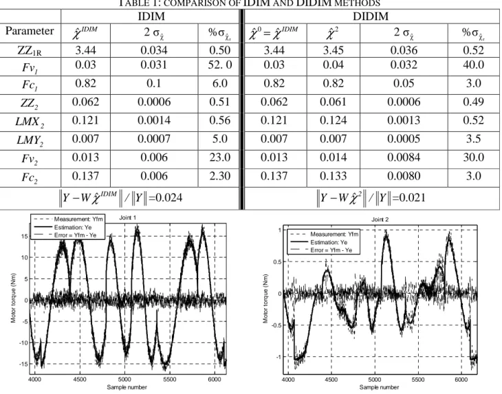
VI. EXPERIMENTAL IDENTIFICATION RESULTS
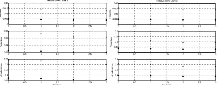
The new identification process is performed in different cases in order to compare the previous IDIM technique to the new DIDIM technique and to investigate the robustness of DIDIM with respect to the initialization, to the acquisition sampling rate, to the data filtering and to the closed-loop tuning.
All the results are given in SI units, on the joint side.
A. Comparison of IDIM and DIDIM with good initial values, χˆ0=χˆIDIM
.
At first, the algorithm is initialized with, χˆIDIM, the vector of parameters identified with the IDIM LS estimator.
This work has been submitted to the IEEE for possible publication. Copyright may be transferred without notice, after which this version may no longer be accessible p 22
The IDIM LS off-line estimation is carried out with a filtered position ˆq , calculated with a 20Hz cut-off frequency forward and reverse Butterworth filter, and with the velocities ˆq& , and the accelerations, ˆq&&, calculated with a central difference algorithm of ˆq . The parallel decimation of Yfm and Wfm, in (10), is carried out with a sample rate divided by a factor, n =20, and a lowpass filter cut-off frequency equal d to, 0.8* /(2*fm nd)=4Hz.
The results are given in Table 1. It needs only 2 steps to obtain the optimal solution which is very close to the IDIM solution. Hence, the DIDIM method does not improve the IDIM solution calculated with good bandpass filtered data.
A validation is plotted on Fig. 10, at the frequency measurement, f =200Hz. It shows that the actual m
joint torques, Yfm
( )
τ , and the torques estimated with the identified model,(
2)
, 2
e fm ddm ddm ddm ˆ ˆ
Y =Wδ q ,q& ,q&& χ χ , as defined in (45), (46), (47), are very close.
Both methods give a small relative norm error, Y −Wχˆ / Y <3%, which shows a good accuracy for the model and for the identified values.
It can be seen that the parameters, Fv , and 1 Fv , have no significant estimations because of their 2 large relative standard deviation (>30%). They have no significant contribution in the joint torques and they can be cancelled to keep a set of essential parameters of a simplified dynamic model, without loss of accuracy [31].
However, we prefer to keep all the parameters in the following, for a better comparison of IDIM and DIDIM identification methods.
This work has been submitted to the IEEE for possible publication. Copyright may be transferred without notice, after which this version may no longer be accessible p 23
TABLE 1: COMPARISON OF IDIM AND DIDIM METHODS
IDIM DIDIM Parameter IDIM ˆ χ 2 σχˆ %σχˆr 0 IDIM ˆ ˆ χ =χ 2 ˆ χ 2 σχˆ %σχˆr ZZ1R 3.44 0.034 0.50 3.44 3.45 0.036 0.52 1 Fv 0.03 0.031 52. 0 0.03 0.04 0.032 40.0 1 Fc 0.82 0.1 6.0 0.82 0.82 0.05 3.0 2 ZZ 0.062 0.0006 0.51 0.062 0.061 0.0006 0.49 2 LMX 0.121 0.0014 0.56 0.121 0.124 0.0013 0.52 2 LMY 0.007 0.0007 5.0 0.007 0.007 0.0005 3.5 2 Fv 0.013 0.006 23.0 0.013 0.014 0.0084 30.0 2 Fc 0.137 0.006 2.30 0.137 0.133 0.0080 3.0 IDIM ˆ Y−Wχ / Y =0.024 Y−Wχˆ2 / Y =0.021 4000 4500 5000 5500 6000 -15 -10 -5 0 5 10 15 Joint 1 M o to r to rq u e ( N m ) Sample number Measurement: Yfm Estimation: Ye Error = Yfm - Ye 4000 4500 5000 5500 6000 -1 -0.5 0 0.5 1 Joint 2 M o to r to rq u e ( N m ) Sample number Measurement: Yfm Estimation: Ye Error = Yfm - Ye
Fig. 10. DIDIM, validation, Ye=Wδfm
(
qddm,q&ddm,q&&ddm,χ χˆ2)
ˆ2.B. DIDIM, validation of the regular initialization, M q( ddm,χˆ0)=I2
The robustness of DIDIM with respect to a wrong initialization, such as the regular initialization (62), is investigated.
The initial values of the dynamic parameters are given by (61), with:
[
]
T1 0 0 1 0 0 0 0
0
ˆ
χ =
The identified values given in Table 2, are very close to those given in Table 1. This result validates the regular initialization procedure , described in section IV.B.