Bank of Canada staff working papers provide a forum for staff to publish work-in-progress research independently from the Bank’s Governing Council. This work may support or challenge prevailing policy orthodoxy. Therefore, the views expressed in this note are solely those of the authors and may differ from official Bank of Canada views. No
Staff Working Paper/Document de travail du personnel — 2020-2
Last updated: January 27, 2020
Social Learning and
Monetary Policy at the
Effective Lower Bound
by Jasmina Arifovic1, Alex Grimaud2, Isabelle Salle3 and Gauthier
Vermandel4
1 Department of Economics Simon Fraser University
Burnaby, British Columbia, Canada [email protected]
2 Department of Economics and Finance Catholic University of Milan, IT, and
Amsterdam School of Economics, University of Amsterdam, NL [email protected]
3 Financial Markets Department Bank of Canada
Ottawa, Ontario, Canada K1A 0G9 [email protected] 4 Paris-Dauphine University, FR and France Stratégie, FR
Page ii
Acknowledgements
The present work has benefited from fruitful discussions and helpful suggestions from Jim Bullard, Ben Craig, Pablo Cuba-Borda, George Evans, Jordi Galí, Tomáš Holub, Cars Hommes, Seppo Honkapohja, Robert Kollmann, Douglas Laxton, Albert Marcet, Domenico Massaro, Bruce McGough, Athanasios Orphanides, Bruce Preston, Jonathan Witmer and Raf Wouters. We also thank the participants of the Workshop on Adaptive Learning on May 7–8, 2018, in Bilbao; the 2018 EEA-ESEM meeting in Cologne; the seminar at the Bank of Latvia on March 23, 2019; the workshop on Expectations in Dynamic Macroeconomic Models at the 2019 GSE Summer Forum in Barcelona; the 2019 Computing Economics and Finance Conference in Ottawa; the 15th Dynare Conference in Lausanne; the 22nd Central Bank Macroeconomic Modeling Workshop in Dilijan, in particular our discussant Junior Maih; the internal seminar at the Bank of Canada on September 22, 2019; and the 2019 SNB research conference in Zurich. This work has received funding from the European Union Horizon 2020 research and
innovation program under the Marie Sklodowska-Curie grant agreement No. 721846, “Expectations and Social Influence Dynamics in Economics.” We thank William Ho for helpful research assistance. None of the above are responsible for potential errors in the paper. The views expressed in the paper are those of the authors and do not necessarily reflect those of the Bank of Canada.
Page iii
Abstract
The first contribution of this paper is to develop a model that jointly accounts for the missing disinflation in the wake of the Great Recession and the subsequently observed inflation-less recovery. The key mechanism works through heterogeneous expectations that may durably lose their anchorage to the central bank (CB)’s target and coordinate on particularly
persistent below-target paths. We jointly estimate the structural and the learning parameters of the model by matching moments from both macroeconomic and Survey of Professional Forecasters data. The welfare cost associated with those dynamics may be reduced if the CB communicates to the agents its target or its own inflation forecasts, as communication helps anchor expectations at the target. However, the CB may lose its credibility whenever its announcements become decoupled from actual inflation, for instance in the face of large and unexpected shocks.
Bank topics: Monetary policy; Monetary policy communication; Credibility; Central bank research; Economic models; Business fluctuations and cycles
1
Introduction
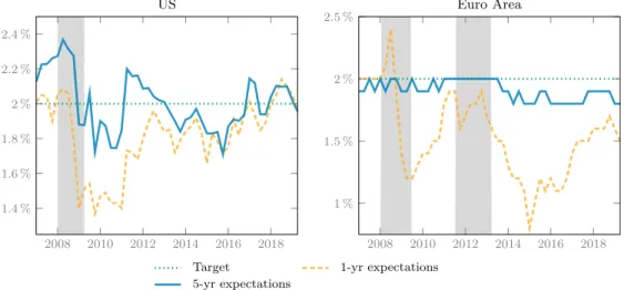
The Great Recession in the US and Europe and the ensuing monetary policy reactions have given way to a ‘new normal’ in economic conditions: interest rates have remained below target. This situation is particularly acute in Europe, where interest rates are still at the effective lower bound (ELB). Yet, no substantial changes in the price levels have been recorded, neither in the wake of the downturn – despite the severity of the recession – nor along the recent output growth episode, which then resembles an inflation-less recovery. Meanwhile, inflation expectations have remained consistently below target, as depicted in Figure 1, which puts at risk the long-run anchorage of expectations. This risk is exacerbated by the structural decline in natural interest rates observed over the last decades, which exerts further downward pressure on inflation expectations (Mertens & Williams 2019). Low inflationary pressures have now pushed a number of major central banks (CBs) to further ease monetary policy.
This low-inflation narrative is hard to unfold within the standard macroeconomic model – namely the New Keynesian (NK) class of models – for at least two reasons.
2008 2010 2012 2014 2016 2018 1.4 % 1.6 % 1.8 % 2 % 2.2 % 2.4 % US
Target 1-yr expectations 5-yr expectations 2008 2010 2012 2014 2016 2018 1 % 1.5 % 2 % 2.5 % Euro Area
Notes: The shaded areas represent the recessions as dated by the National Bureau of Economic Research (NBER) and Centre for Economic Policy Research (CEPR), and the green dashed lines the inflation targets. Data are from the Survey of Professional Forecasters (SPF) and the European Central Bank (ECB).
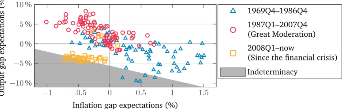
−1 −0.5 0 0.5 1 1.5 −10 % −5 % 0 % 5 % 10 %
Inflation gap expectations (%)
Output gap expectations (%) 1969Q4–1986Q4 1987Q1–2007Q4 (Great Moderation) 2008Q1–now
(Since the financial crisis) Indeterminacy
Notes: The shaded area denotes the region of the state space that violates the determinacy condition under rational expectations (REs) in the sense ofBlanchard & Kahn(1980) and leads to diverging deflationary spirals under recursive learning. In contrast, the white area denotes the region of the state space that is determinate, which is also the basin of attraction of the target under recursive learning. Data on expectations are taken from the Survey of Professional Forecasters. The output gap is computed using a linear trend. Calibration of the New Keynesian model is taken from
Gal´ı(2015).
Figure 2: (Ir)relevance of the New Keynesian model with rational expectations since the ‘new normal’
First, zero interest rates generate implausible macroeconomic dynamics in those mod-els. Under rational expectations (RE), the dynamics are indeterminate at the ELB (Benhabib et al. 2001), which implies excess volatility in inflation that is clearly at odds with the recent experience. This puzzle is clearly visible from survey data, which have been lying in the indeterminacy region of the inflation-output state space since the financial crisis, as depicted in Figure 2. Replacing RE by boundedly rational and learning agents induces diverging deflationary spirals at the ELB, which does not match the current situation either (Evans et al. 2008).
Second, the standard assumption of complete information and common beliefs leaves little room for expectations to be persistently off the target and play any autonomous role in driving business cycles. In those models, recessive episodes are typically gen-erated by exogenous and persistent technology or financial shocks.1 Not only does
this conception of expectations conflict with the empirical evidence of unanchored and 1There are some recent exceptions, e.g. Angeletos et al.(2018), who investigate the role of strategic uncertainty in the presence of heterogeneous information within a general equilibrium model. However, those authors use a real business cycle (RBC) model, which implies that monetary policy is left out.
dispersed forecasts that has been found in survey data,2 but it also does not leave any room for monetary policy to influence or coordinate private expectations through communication.
Therefore, the main contribution of this paper is to address these challenges by developing a model in which time-varying and persistent heterogeneity in expectations endogenously produces ELB dynamics so as to account for the recent economic expe-rience. The use of heterogeneity and learning in agents’ expectations is not anecdotal given the large literature documenting deviations from RE in real-world expectations and, in particular, pervasive and time-varying heterogeneity.3 Heterogeneity in expec-tations also poses a challenge to the CB when attempting to coordinate the private sector on the desirable inflation target. Moreover, forecast dispersion has been directly related to macroeconomic uncertainty (Rossi & Sekhposyan 2015) and has been proven to induce adverse effects on the economy (Jo & Sekkel 2019).
Specifically, we develop a micro-founded NK model featuring inflation and output dynamics to which we add a parsimonious two-operator evolutionary learning process that specifies the dynamics of expectations and nests the RE homogeneous agent bench-mark. This latter feature, together with the sole use of white noise fundamental shocks, isolates learning as the only possible source of persistence in the endogenous variables and allows us to identify the amplifier role of expectations in driving business cycles. In our model, agents form beliefs about the long-run values of inflation and output. This easily translates into the issue of expectation anchorage. Our choice of a social learning 2For instance, using survey data, Coibion et al.(2019) show that more than half of the firms and households typically do not know the value of the Fed inflation target, while only 20% of them pick the correct answer. Using the Michigan Survey of Consumers,Coibion et al.(2018) find that one-year-ahead households’ expectations are on average 1.5 percentage points (p.p.) above the 2% target of the Fed. The cross-sectional dispersion is also large, up to 3 p.p. in March 2018. Furthermore, Coibion et al. (2018) show that making information salient, notably by providing announcements that are sufficiently clear for the general population, allows the CB to curb inflation expectations and therefore real interest rates.
3On deviations from RE in general, we refer to, inter alia,Mankiw et al.(2003),Del Negro & Eusepi (2011) andBranch(2004). On heterogeneity in particular, see, e.g.,Hommes(2011) for evidence using lab forecasting experiments; Mankiw et al. (2003) in survey data from professional forecasters; and
(SL) process is motivated by the parsimony of this class of learning models, their ability to match experimental findings and the evolutionary role of heterogeneity in the adap-tation of the agents (Arifovic & Ledyard 2012). In these models, agents collectively adapt to an ever-changing environment in which their own expectations contribute to shape the macroeconomic variables that they are trying to forecast. Specifically, SL agents dynamically improve their individual forecast strategy through stochastic explo-ration and imitation of other agents with better historical accuracy in their forecasts. Per consequence, optimistic or pessimistic agents’ strategies drive aggregate expecta-tions during booms or busts thanks to their improved accuracy. This feature is well suited to self-referential economic systems such as standard macroeconomic models. SL expectations also find an intuitive interpretation that is reminiscent of the idea of epidemiological expectations where ‘expert forecasts’ only gradually diffuse across the entire population (Carroll 2003).
In a novel effort within the related literature,4 we take our stylized model to the data
and show that it is able to jointly replicate ten salient business cycle moments from the Survey of Professional Forecasters (SPF) and the main US macroeconomic time series, including the frequency of ELB episodes, major dimensions of heterogeneity in expectations and a substantial share of the persistence in output and inflation data.
This empirical exercise is already a remarkable result given the parsimony of the model. Yet, it is important to note that we do not aim to contrast the matching abilities of the SL model regarding macroeconomic time series with those of an RE counterpart. For a fair comparison, the SL model would need to compete with an RE version of the model with sunspot dynamics at the ELB. While certainly a needed exercise, it is beyond the scope of the present paper. What our empirical exercise 4Del Negro & Eusepi (2011) attempt to replicate expectation data with RE models. Milani(2007) fits an adaptive learning NK model to macroeconomic time series only. Closer to our contribution,
Slobodyan & Wouters(2012a,b) fully estimate an NK model on both macroeconomic and expectations times series. However, the authors use exogenous autocorrelated shocks on expectations to reproduce the observed persistence in the data.
does add to the literature is (i) an estimation routine of a non-linear model under heterogeneous expectations and (ii) an empirical discipline device to learning models by offering estimated values to the learning parameters for which there are no observable counterparts.5
A second major contribution is to show that our model endogenously produces stable dynamics at the ELB. Those stable dynamics correspond to inflation-less recoveries, i.e. inflation persists for an extended period of time below its target, the ELB binds, but output expands.6 Such a configuration corresponds to the recent economic experience. This means that our simple framework can jointly account for the missing deflation in the wake of the crisis and the missing inflation in the wake of the recovery. In our model, recessive dynamics arise endogenously when agents coordinate on pessimistic expectations following a series of adverse but non-autocorrelated shocks. From there, the transition back to the target can be particularly long if expectations have become unanchored and, per their self-fulfilling nature, nurture the bust. Hence, we offer a reading of the recent economic experience as a long-lasting coordination of agents on pessimistic expectations rather than as the result of persistent and exogenous financial or technological shocks. The forces underlying our narrative are reminiscent of the earlier Keynesian concept of animal spirits.
Furthermore, we introduce central bank communication as a welfare-enhancing tool to coordinate heterogeneous expectations. Given that our model nests the RE homogeneous-agent benchmark, we interpret the dispersion of expectations as a fric-tion and quantify the ensuing welfare loss with respect to the RE outcome. We find that heterogeneous expectations entail a consumption loss of almost 3.3% with respect to the RE allocation. This highlights how crucial heterogeneity in expectations is with 5The usual practice in the learning literature is to rely on calibrated models with no quantitative assessment of their empirical relevance in terms of replication of business cycle moments.
6The following result would also hold in the presence of unconventional monetary policy captured by a shadow interest rate falling beyond zero and a larger output expansion.
respect to the representative agent construction of the standard NK model. From there, a natural follow-up analysis is to introduce an additional monetary policy instrument next to the interest rate, namely CB communication, and investigate whether it may offset the costs of forecast dispersion and deliver the RE representative agent bench-mark. To address this question, we exploit the flexibility of our parsimonious learning model, which enables us to integrate CB communication into the learning process of the agents. We show that announcing the inflation target or inflation forecasts may help enforce coordination of agents’ expectations on the target. As coordination on pessimistic outlooks is the source of the aggregate propagation of shocks in our model, CB communication reduces the occurrence as well as the severity of ELB episodes and cuts the welfare loss due to heterogeneous expectations, which brings the CB closer to, but nonetheless below, the RE outcome. However, in the face of large unexpected shocks, the CB may lose credibility whenever the announcements become decoupled from the actual realizations of inflation.
Related literature Our treatment of communication adds to the existing literature on communication under learning by modeling endogenous credibility.7 The closest to our concept of endogenous credibility is the work byHommes & Lustenhouwer (2019), who derive the stability conditions of the targeted equilibrium in an NK model with ELB where agents’ expectations switch to follow past inflation, should the target be missed.
A rapidly expanding literature on Heterogeneous Agent New Keynesian (HANK) models investigate the consequences of heterogeneous agents on monetary policy design (see, for a recent account, Gal´ı(2018) and the references herein). While this literature is mostly concerned with the aggregate effects of idiosyncratic shocks on households’ 7The learning literature usually concludes that communication is stabilizing under learning in mod-els where communication imposes model-consistent restrictions on the forecasting model used by the learning agents; see e.g. Eusepi & Preston(2010). However, a crucial assumption in these models is that communication is credible.
income, we model heterogeneity in expectations. Their implementation of heterogeneity also results in models that are considerably more complicated than ours, as it requires, among other challenges, keeping track of the wealth distribution over time.
In addition, our work substantially differs from New Keynesian models with multiple equilibria where a liquidity trap episode is understood as an exogenously driven regime switch from the targeted equilibrium to the deflationary steady-state (Aruoba et al. 2017, Jaroci´nski & Ma´ckowiak 2018). While we also aim to explain the persistent slump after the Great Recession, we do so by using a learning model under which the basin of attraction of the target is larger than the determinacy region under RE. In the context of our model, expectations formed by the learning agents may occasionally visit regions of that basin from where the transition back on target is particularly slow. Those shifts in expectations arise because the interplay between SL and fundamental shocks may cause agents to ‘pick up’ a downward trend in inflation and output gaps following a series of bad shocks, rather than as a result of the use of sunspots as expectation coordination devices. Schmitt-Groh´e & Uribe (2017) consider exogenous confidence-driven rather than sunspot-confidence-driven regime changes but do not model the unanchoring process of expectations from the target. Furthermore, we add to this literature the treatment of communication and endogenous credibility of the CB’s announcements.
We borrow from Arifovic et al. (2013, 2018) a similar SL mechanism to model expectations within a NK model. However, our present work differs along important dimensions. Among others, those two contributions study the long-run stability of the model as defined by the asymptotic convergence towards a particular equilibrium under SL, while we focus on the short-term fluctuations arising from the interplay between fundamental shocks and learning dynamics. None of those models are taken to the data, and only Arifovic et al. (2018) introduce the ELB but use exogenous shocks to trigger liquidity trap episodes. Those authors interpret such episodes as the anchoring of expectations on the low inflation steady-state, which is not, as explained previously,
the mechanism generating liquidity traps in this paper. In other words, in our model, we do not contemplate the possibility of the deflationary steady-state to be an attractor of the learning process. WhileArifovic et al.(2018) show that the low inflation steady-state may be a stable attractor of their SL mechanism, our implementation of the fitness function and our empirical calibration differ from theirs, which does not allow us to generalize their result to our setup. Furthermore, Arifovic et al. (2013, 2018) do not consider CB communication and do not measure the welfare implications of that departure from RE.
The rest of the paper proceeds as follows. In Section 2, we develop the model; the estimation is presented in Section3; the dynamic properties of the model are analyzed in Section4; Section5discusses the effects of CB communication; and Section6concludes.
2
The model
We first describe the building blocks of the model, then we discuss the solution under the RE benchmark and finally explain our implementation under SL.
2.1
A piecewise linear New Keynesian model
Our model builds on the workhorse three-equation NK model developed by, inter alia,
Woodford (2003). The three equations describe aggregate demand, aggregate supply and monetary policy. All variables below are expressed in deviation from their steady-state level as targeted by the CB.
Aggregate demand is described by the IS curve:
b yt= E∗j,tybt+1− σ −1 (bıt− E ∗ j,tπbt+1) +gbt, (1)
of the inflation rate from the target (hence, bıt − Etπbt+1 represents the real interest rate), σ > 0 the inter-temporal elasticity of substitution of consumption (based on a CRRA utility function), and E∗j,tthe (possibly boundedly rational) expectation operator
based on information available at time t. The subscript j is introduced to suggest the possibility of heterogeneous expectations, where each agent-type j = 1, ..., N forms her own expectation (with N the number of agent-types).8
b
g is an exogenous real disturbance.
The supply side is summarized by the forward-looking NK Phillips Curve:
b
πt= βE∗j,tπbt+1+ κybt+cut, (2)
where 0 < β < 1 represents the discount factor, κ > 0 a composite parameter capturing the sensitivity of inflation to the output gap andcut an exogenous cost-push shock.
In the RE literature, the shocksg andb u are usually assumed to be AR(1) processes:b
b gt =ρggbt−1+ ε g t, (3) b ut =ρuubt−1+ ε u t, (4)
where 0 ≤ ρu, ρg < 1 measure the persistence of the shocks and εg, εu are i.i.d. with
respective standard deviations σg and σu.
Monetary policy implements a flexible inflation-targeting regime subject to the ELB constraint, which results in the following non-linear forward-looking Taylor rule:
b
ıt= max{−r; φπE∗j,tπbt+1+ φ
y
E∗j,tybt+1}, (5)
8We follow here most of the learning literature and introduce heterogeneity in the reduced-form models rather than in the micro-foundations (see, inter alia,Bullard & Mitra (2002),Arifovic et al.
(2013), Hommes & Lustenhouwer (2019)). We are well aware of the conceptual limitation of this approach. Nonetheless, while the complications of the alternative are clear (see e.g. Woodford(2013)), the benefits in terms of qualitative results remain uncertain. For instance, in an asset-pricing model,
Adam & Marcet(2011) show that under a sophisticated form of adaptive learning, the infinite-horizon pricing equation reduces to a myopic mean-variance equation. Bearing in mind those caveats, we proceed within the reduced-form model.
where φπ and φy are, respectively, the reaction coefficients to the inflation and the output gaps, and r ≡ πT + ρ the steady-state level of interest rate associated with the inflation target πT and the households’ discount rate ρ ≡ − log(β).
We now solve the model under the benchmark of RE and then detail how we intro-duce SL in the expectation formation process of the agents.
2.2
The model under rational expectations
In this section, we consider RE and impose E∗j,t(·) = E(· | It) to be the rational
expectation operator given the information set It common to all agents in period t. We
solve for the Minimal State Variable (MSV) solution using the method of undetermined coefficients.
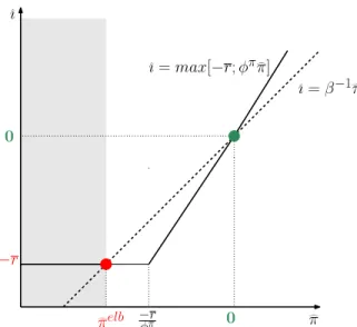
It is well known that the ELB introduces a non-linearity in the Taylor rule and generates an additional deflationary steady-state next to the target (Benhabib et al. 2001). This ELB steady-state corresponds to a liquidity trap where the deflation rate matches the discount factor. Hence, expressing the model in reduced form is challenged by this non-linearity, and we need to disentangle two pieces, one around the target and one when the ELB is binding.9
A short digression through the one-dimensional Fisherian model easily illustrates this configuration. Figure 3 displays inflation and interest rate dynamics, abstracting from the production side: the social optimum or inflation target corresponds to π = 0b and the deflationary steady-state toπb
elb. Provided that
b
πelb ≤ 0 ≤ πT, the two equilibria
co-exist.
9We follow here the related NK literature and impose the ELB constraint in the log-linearized model around the targeted steady-state to describe the dynamics around the low inflation state, see,
inter alia,Nakov(2008), Guerrieri & Iacoviello(2015). This method gives a second-best estimate of the dynamics around the deflationary steady-state. A first-best would be to log-linearize the model around this second steady-state but would result in an MSV solution involving extra additional state variables (Ascari & Sbordone 2014) and, hence, additional coefficients to learn under SL (see Section
2.3). However, the benefits in terms of qualitative results are unlikely to outweigh the costs of such a complication of the learning process of the agents.
0 −r b ı = β−1dπ b ı = max[−r; φπdπ] d πelb −rφπ b ı d π 0
Notes: We can write the log-approximated Fisher equation as follows:bı = β−1bπ. At the targeted steady-state (in green),
no deviation occurs: bı = β−1
b
π = 0. At the ELB (in red), we can derive an equilibrium such that −r = β−1
b
πelb ⇔ bπ
elb = −rβ. Provide that b
πelb ≤ πT, the two equilibria co-exist. The shaded area is indeterminate under RE and
unstable under adaptive learning (Evans et al. 2008).
Figure 3: Co-existence of two steady states under the ELB constraint
Coming back to the two-dimensional model, AppendixA shows that the functional form of the Minimal State Variable-Rational Expectation Equilibrium (MSV-REE) at the target reads as:
zt= (ybt πbt)
0 = a + c
b
gt+ dubt. (6)
The expression of the matrices a, c and d depends on the steady-state considered. In the rest of the paper, we consider white noise shocks, i.e. ρg = ρu = 0, so the
disturbances u and g are i.i.d. processes. We assume that u and g are not observable. In this case, the REE solution (6) boils down to a noisy constant a without endogenous persistence. The presence of a floor on the nominal rate makes the equilibrium law of motion of the economy piece-wise:
zt = [ybt πbt] 0 = aT + χg b gt+ χuubt, if it> 0 aelb+ χg b gt+ χuubt, if it= 0, (7)
a ‘T’ superscript), the second case is when the ELB is binding (denoted by a ‘elb’ superscript), aT = (I − BT)−1αT, aelb = (I − Belb)−1αelb. In the latter expressions, I
is the 2-by-2 identity matrix while α, B, χg and χu are matrices from the solution of
the rational expectation model. The exact expression of these matrices can be found in Appendix A. Note that as variables are normalized with respect to their steady-state values at the target, we have aT = (0 0)0. We now introduce the expectation formation
mechanism under SL.
2.3
Expectations under social learning
Under SL, we relax the assumption of homogeneous agents endowed with RE and consider instead a population J of N heterogeneous and interacting agents, indexed by j = 1, · · · , N . We now define E∗j,t(·) = EjSL(· | Ij,t) to be the expectation operator
under SL given the information set Ij,t available in period t to agent j. The information
set is agent specific as it contains, besides the history of past inflation and output gaps up until period t − 1, the current and past individual forecasts that need not be shared with the whole population. Figure4 summarizes the intra-period dynamics under SL. We now detail each step.
Individual forecasting rules FollowingArifovic et al.(2013,2018), we assume that agents are endowed with a forecasting rule that involves the same variables as the MSV solution. The form of the rule is the same across agents, but with agent-specific coefficients that they revise over time. In any period t, each agent j is therefore entirely described by a two-component strategy [ayj,t, aπ
j,t]
0 and her expectations read as:
Ej,tSL{ˆzj,t+1} = ESL j,t {ˆyt+1} ESL j,t {ˆπt+1} = ayj,t aπ j,t . (8)
Fitness computation (Eq. 11) Updated expectations {ayj,t+1, a π j,t+1} i.i.d. shock realisation εgt, εut Aggregation of individual expectations (Eq. 9) Computation of endogeneous variables (Eqs. 5-1-2) Mutation of individual expectations (Eq. 10) Tournament selection (Eq. 12) t +06 t +06 t +t +t +06006 t +06 6 t +1 6 t + t + 1 0 6 t +2 6 t +2 6 t + 0 6 t +3 6 t + 4 6 t + 5 6
Figure 4: Intra-period timing of events in the model under SL
Those pairs of forecast values find an appealing interpretation. In the absence of shocks, ayj corresponds to her long-run output gap forecast and aπj to her long-run inflation gap forecast. In the presence of i.i.d. shocks, those values correspond to her average output gap and inflation gap forecasts. Under either of those interpretations, the forecasts [ayj,t aπ
j,t]
0 of the agents represent their beliefs about the steady-state values of the
infla-tion and output gaps, which allows us to intuitively measure expectainfla-tion anchorage or unanchorage by simply evaluating the distance between those forecasts values, and their targeted counterparts (i.e. zero).10 On empirical grounds, heterogenous coefficients
[ayj,taπ
j,t] may also capture the disagreement among forecasters observed in survey data.
In particular, dispersed coefficients on inflation aπj,t can be interpreted as disagreement about the CB target, as the latter typically coincides with the inflation steady-state in the workhorse NK model. This disagreement has been empirically documented by surveys conducted byCoibion et al. (2018) for both firms and households in the US.
10In the sequel, we denote by Ω such an indicator of expectation anchorage. Specifically, we use the average squared distance of individual expectations to zero: ΩEπ
t = N1 PN j=1E SL j,t {πbt+1} 2 and ΩEy t = 1 N PN j=1E SL j,t {byt+1} 2
Aggregation of individual forecasts Following furtherArifovic et al.(2013,2018), individual expectations (8) are aggregated using the arithmetic mean as:
EtSLzbt+1 = 1 N N X j=1 ESLj,tzbt+1, (9)
and inserted into the reduced-form model (17) to obtain the dynamics of the endogenous variables under SL. Under this aggregation procedure, agents have the same relative weight in expectations formation, thus one agent cannot influence market expectations if the number of agents N is large enough. To have a sizable effects on market expecta-tions, a sentiment or news must spread to a large enough fraction of the population to generate expectation-driven fluctuations. We now detail how agents interact and how their forecasts evolve as sentiments to diffuse in the population.
Agents collectively explore the space of possible forecast values [ ay aπ]0. Specifically,
this class of learning models utilizes two operators.
Mutation The first one is a stochastic innovation process, or mutation, that allows for a constant exploration of the state space outside the existing population of forecasts. In each period, each agent’s forecasts are modified by an idiosyncratic shock with ex-ogenously given probabilities. Her output gap forecast is modified with probability µy
and her inflation gap forecast with probability µπ. In short, her forecasts of any variable
x = {y, π} modified in any period as follows:
axj,t+1 = axj,t+ ιj,tξx with probability µx axj,t with probability 1 − µx, (10)
with ιj,t an idiosyncratic random draw from a standard normal distribution with
stan-dard deviation ξx. In other words, mutations occur in the neighborhood of the indi-vidual strategies, and the size of this neighborhood is directly tuned by parameter ξy along the output dimension and ξπ along the inflation dimension. The larger those
parameters, the wider the neighborhood to be explored around the existing strategies ayj,t and aπj,t. Mutation can be interpreted as an innovation, a trial-and-error process or a control error in the computation of the corresponding expectations.
Tournament and computation of forecasting performances The second oper-ator, the tournament, is the selection force of the learning process and allows better-performing strategies to spread among the population at the expense of lower-better-performing ones. Performance of any forecasting rule [ayj,t, aπ
j,t]
0 is evaluated using the forecast
er-rors over the whole past history of the economy (not solely over the last period) given the stochastic nature of the environment (seeBranch & Evans 2007).
For each agent j, her forecast axj,t of each variable x = {y, π} is assessed regarding forecast errors. To each strategy ax
j,t is assigned a so-called fitness, computed as:
Fj,tx = − t X τ =0 (ρx)τ(xbt−τ − a x j,t) 2. (11)
The termsybt−τ−a
y
j,tandπbt−τ−a
π
j,t correspond, respectively, to the output and inflation
gap forecast errors that agent j would have made in period t − τ − 1, had she used her current forecast values ayj,t and aπ
j,t to predict the output and inflation gaps in period
t − τ . The smaller the forecast errors, the higher the fitness.
Parameter ρx ∈ [0, 1] (for x = y, π) represents memory. In the nested case where
ρx = 0, the fitness of each strategy is completely determined by the forecast error on the most recent observable data, i.e. t given our timing of events (see, again, Fig. 4). For any 0 < ρx ≤ 1, all past forecast errors impact the fitness but with exponentially
declining weights while, for ρx = 1, all past errors have an equal weight in the
compu-tation of the fitness. This memory parameter allows the agents to discriminate between a one-time lucky draw and persistently good forecasting performances.
In the tournament, agents are randomly paired (the number of agents is conveniently chosen even), their fitness on inflation and output gap forecasts are each compared and
the one with the lowest fitness copies the forecast of the other. There are two separate tournaments: one for inflation gap forecasts {aπj,t}j∈J and one for output gap forecasts
{ayj,t}j∈J. Formally, for each pair of agents k, l ∈ J , k 6= l, with individual forecasts
ax
k,t and axl,t (x ∈ {π, y}), the tournament operates an imitation of the more successful
forecasts as follows:
axk,t+1 = axl,t+1 = axk,t if Fk,tx > Fl,tx axk,t+1 = ax
l,t+1 = axl,t if Fk,tx ≤ Fl,tx
, for x ∈ {π, y}. (12)
The tournament occurs after the mutation operator in order to screen out bad-performing forecasts stemming from mutation. This allows the model to be less sensitive to the parameter values tuning mutation (i.e. the probabilities µx and the size ξx,
x = {y, π}) than if mutation were to take place after the tournament selection, and all newly created forecasts were to determine aggregate expectations without consideration of their performances. This way, the mutation process can be more frequent and of wider amplitude so as to allow for a faster adaptation of the agents to new macroeconomic conditions, while limiting the amount of noise introduced by the SL algorithm.
Simulation protocol We study the dynamics of the model using numerical simu-lations. Throughout the rest of the paper, we proceed as described in Arifovic et al.
(2013, 2018). We generate a history of 100 periods along the law of motion of the economy around the target (see Eq. (7)) and introduce a population of SL agents in t = 100. Their initial forecasts are drawn from the same support as the one used in the mutation process, i.e. from a normal distribution with standard deviation ξx, x = π, y. The first 100 periods are used to provide the agents with a history of past inflation and output gaps in order to compute the fitness of their newly introduced forecasts. In the simulations exercises in the next sections, we vary the initial average of the normal distribution to tune the degree of pessimism in the economy. The further below zero the
initial average forecasts are, the more pessimistic views the agents hold about future inflation and output gaps.
Finally, it is important to recognize that the RE representative agent benchmark is nested in our heterogeneous-agent model: as soon as the inflation and output gap expectations of all agents are initialized at the targeted values and mutation is switched off (i.e. ξy, ξπ = 0), the dynamics boil down to the RE benchmark. Under SL, our
model involves a few parameters, namely the probabilities of mutation, the sizes of those mutations and the memory of the fitness function. We now detail how we estimate those parameter values.
3
Estimation of the model under social learning
We jointly estimate the learning parameters and the structural parameters of the model. We first describe our choice and construction of the dataset, then discuss our estimation method and, finally, present the results.
3.1
Dataset
Macroeconomic US time series for output, price index and nominal rates are taken from the FRED database. Forecast data come from the SPF of the Federal Reserve of Philadelphia. This choice is usual in the related literature, as it is argued that those data provide a good approximation of the private sector expectations that are implicitly involved in the New Keynesian micro-foundations (Del Negro & Eusepi 2011). SPF data span the period from 1968 to 2018 on a quarterly basis. To make the dataset stationary, we divide output by both the working age population and the price index. In order to obtain a measurement of the output gap, we compute the percentage deviations of the resulting output time series from its linear trend. The inflation rate is measured by the growth rate of the GDP deflator.
As heterogeneity in expectations drives the dynamics of the SL model, we construct
an empirical measure of that heterogeneity in the survey data. We use the
cross-sectional dispersion of the individual forecasts in order to obtain time series of forecasts’ heterogeneity and compute the standard deviation of the individual forecasts among all participants in each period of the survey.
3.2
Estimation method
With those data at hand, we proceed by matching the statistics from empirical mo-ments with their simulated counterparts under SL. We provide technical details of our
estimation method in Appendix C. In short, we use the Simulated Moments Method
(SMM) as initially developed by McFadden(1989), which provides a rigorous basis for evaluating whether the model is able to replicate salient business cycle properties.11
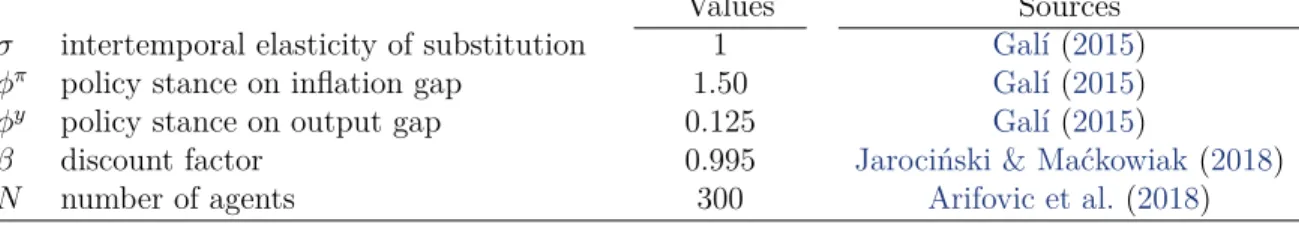
In order to avoid identification issues, the number of estimated parameters has to be equal to the number of matched moments so that each estimated parameter can be directly mapped onto one empirical moment. Hence, we first have to reduce the number of dimensions of the matching problem and calibrate some of the parameters, namely the monetary policy and the preference parameters, as is standard in the related macroeconomic literature, and the number of agents (see Table1).
We are left with four structural parameters from the NK model, namely the size of the fundamental shocks σg and σu, the slope of the NK Phillips curve (parameter κ) and the natural rate r. As we have calibrated the value of the discount factor β (see Table1), we estimate the value of the inflation trend over the period considered, which uniquely determines the value of ¯r.12 As for the SL parameters, we need not estimate 11Due to the non-linearity introduced by the ELB, we may not apply the Kalman filter and would need to use a non-linear filter to estimate the model with Bayesian full-information techniques. Given that this paper is the first attempt to bring such a heterogeneous-expectation model to the data, we encountered additional difficulties in estimating the SL model with an SMM (see Appendix C). In particular, the SL algorithm brings an additional non-linearity into the piecewise-linear model and an additional source of stochasticity next to the fundamental shocks. Hence, we have left the perspective of Bayesian estimation for future research.
Values Sources
σ intertemporal elasticity of substitution 1 Gal´ı(2015)
φπ policy stance on inflation gap 1.50 Gal´ı(2015)
φy policy stance on output gap 0.125 Gal´ı(2015)
β discount factor 0.995 Jaroci´nski & Ma´ckowiak(2018)
N number of agents 300 Arifovic et al.(2018)
Table 1: Calibrated parameters (quarterly basis)
common values for the inflation and the output gap expectation processes as the two tournaments are separated and the two time series are likely to behave differently and exhibit different properties, both in reality and in the model. For instance, estimating inflation and output gap-specific memory parameters ρπ and ρy may translate the fact that agents can learn that one variable may display more persistence than the other. Hence, we estimate six learning parameters, namely the mutation sizes and frequencies ξx and µ
x as well as the memory of the fitness measures ρx for x = {π, y}.
We now discuss the mapping between those parameters and the empirical moments to match. First, the standard deviations of the shocks σg and σu naturally capture
the empirical volatility of output and inflation. Second, the inflation trend π aims to match the ELB probability. To see why, recall that a higher natural rate ¯r mechanically decreases the probability of hitting the ELB, as the latter is defined asıbt = −¯r, which is strictly decreasing in the value of the inflation target. Finally, the slope of the Phillips curve κ determines the correlation between the output and inflation gaps per Eq. (2). As for the SL parameters, the memories of the fitness function ρy and ρπ tune the
sluggishness of the expectations because they determine the weights on recent versus past forecast errors in the computation of the forecasting performances. The higher ρy and ρπ, the longer the memory of the agents, the less reactive the learning process to recent errors and the more sluggish the expectations. As sluggishness in expectations is the only source of persistence in the model once we consider i.i.d. shocks, parameters in the US for most of the time period considered. Therefore, we estimate an inflation trend over that period.
ρy and ρπ are matched with the autocorrelation of, respectively, the output and the inflation gaps.
The remaining four learning parameters control the mutation processes that are the source of the pervasive heterogeneity in expectations in the SL model. We understand-ably use those parameters to match four moments characterizing heterogeneity in the SPF data: the average dispersion of the output and the inflation gap forecasts over the time period considered, denoted respectively by ∆Ey and ∆Eπ, and their first-order
autocorrelations, denoted by ρ(∆Ey
t , ∆Eyt−1) and ρ(∆Eπt , ∆Eπt−1). In line with intuition,
sensitivity analyzes of the objective function of the matching problem with respect to those learning parameters have reported the following associations: the mutation sizes ξy and ξπ capture a substantial share of the empirical dispersion of output and
in-flation gap forecasts, while the mutation frequencies µy and µπ match most of their
autocorrelation.
Finally, in the same vein asRuge Murcia(2007), we impose prior restrictions on the estimated parameters and treat them as additional moments in the objective function. The details are deferred to AppendixC. The priors for the structural NK parameters are taken from the literature on Bayesian estimation of DSGE models (Smets & Wouters 2007) and we choose priors for the learning parameters that are in line with the values used in the SL literature such asArifovic et al. (2013) (see Table 3).
3.3
Estimation results
Table 2 reports the matched moments and their empirical counterparts (in percentage points). Table 3 gives the corresponding estimated values of the parameters.
It is first striking to see how the simple two-dimensional model delivers remarkably good matching performances along the ten stylized facts considered. The estimated model accounts for a substantial share of all ten moments. For half of them, the simu-lated moments even fall within the confidence interval of their empirical counterparts,
which means that our model replicates those moments fully. We succeed in capturing not all, but a non-negligible part, of the persistence in macroeconomic variables with a model that employs only white-noise shocks.13 We shed further light on the source
of that persistence in Section4.1, but at that stage, we can state that learning acts as an endogenous propagation mechanism that amplifies the effects of i.i.d. shocks and accounts for 22% of the empirical output gap persistence and even 63% of the inflation persistence found in the data.
Furthermore, all simulated correlations are of the same sign as their observed coun-terparts. Our model succeeds in producing positive autocorrelation in forecast disper-sion. This result is an important step forward in the modeling and estimation literature as we show that our simple framework can address the empirical heterogeneity in ex-pectations that is not part of the RE material.
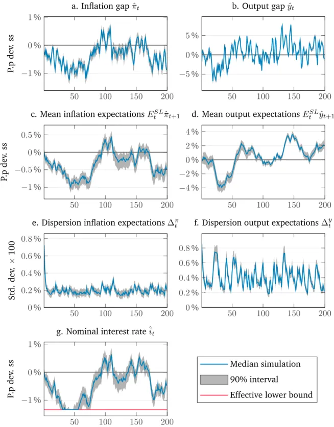
The model also matches particularly well the probability of the ELB on nominal interest rates to bind despite the relatively modest amplitude and i.i.d. structure of the fundamental shocks. Those ELB episodes are not the result of large exogenous shocks but are an endogenous product of the interplay between learning and those small i.i.d. shocks. For illustrative purposes, Figure 5 displays the time series of the endogenous variables and the expectations from a representative simulation of the model. We can see an occasionally binding ELB around periods 30 to 60 that coincides with below-target expectations. Before detailing in the next section how such dynamics can arise from the amplification mechanism induced by SL, we briefly discuss the estimated values of the parameters inTable 3.
All our estimated values are consistent with empirical values and usual estimates. For instance, the estimated value of the slope of the Phillips curve (κ) is in line with 13Matching all the persistence would not be a realistic or desirable objective: it is unlikely that all macroeconomic persistence stems from learning in expectations and our model ignores all other fundamental sources of persistence in the economy. We rather provide a measure of the share of the persistence that can be attributed to learning.
Moments Empirical
Matched moments Empirical MO Simulated MS Conf.int.
σ(ˆyt) - output gap sd. 4.38 4.39 [3.97 - 4.83]
ρ(ˆyt, ˆyt−1) - output gap autocorr. 0.98 0.22 [0.98 - 0.99]
σ(ˆπt) - inflation gap sd. 0.6 0.66 [0.54 - 0.66]
ρ(ˆπt, ˆπt−1) - inflation gap autocorr. 0.9 0.56 [0.87 - 0.92]
ρ(ˆπt, ˆyt) - inflation-output correlation 0.08 0.097 [-0.07 - 0.21]
∆Ey - av. forecast dispersion of output gap 0.36 0.4 [0.31 - 0.41]
∆Eπ - av. forecast dispersion of inflation gap 0.25 0.20 [0.22 - 0.28]
ρ(∆Ey
t , ∆Eyt−1) - autocorr. of forecast disp. of output gap 0.76 0.63 [0.70 - 0.82]
ρ(∆Eπ
t , ∆Eπt−1) - autocorr. of forecast disp. of inflation gap 0.64 0.4 [0.55 - 0.72]
P (it> 0) - probability not at the ELB 0.86 0.83 [0.81 - 0.91]
Objective function × 0.85 ×
Notes: The values in brackets are the confidence interval at 99% of the empirical moments.
Table 2: Comparison of the (matched) theoretical moments with their observable coun-terparts
Prior Distributions Posterior Results
Estimated Parameters Shape Mean STD Mean STD
σg - real shock std Invgamma .1 5 3.8551 5.1e-06
σu - cost-push shock std Invgamma .1 5 0.4232 4.1e-06
π - quarterly inflation trend Beta .62 .1 0.829 7.7e-06
κ - Phillips curve slope Beta .05 .1 0.0095 4e-06
µy
-mutation rate for Ey Beta .25 .1 0.2467 4.6e-06
µπ - mutation rate for Eπ Beta .25 .1 0.2748 6e-06
ξy - mutation std. for Ey Invgamma .1 2 0.8547 3.3e-06
ξπ
-mutation std. for Eπ Invgamma .1 2 0.7406 1.9e-06
ρy
-fitness decay rate for Ey Beta .5 .2 0.8301 9.4e-06
ρπ
-fitness decay rate for Eπ Beta .5 .2 0.5465 5.4e-06
Notes: The low values of the standard deviation of the estimated parameter values only indicate that the algorithm has converged; they do not translate into confidence intervals.
Table 3: Estimated parameters using the simulated moment method matching the SPF data (1968–2018)
Woodford (2003) and is also consistent with the structural flattening underlying the most recent measures (Gourio et al. 2018). The estimated (yearly) inflation trend is 3.4%, which nicely falls into the range between the average inflation rate over the time span considered that includes the 1970s (4.3%) and the Fed inflation target that was adopted later (2%). Next, given the calibrated discount factor β, the implied value for the (yearly) natural interest rate is 5.45%, which is close to the average federal funds rate over the sample (namely 5.2%).
50 100 150 200 −1 % 0 % 1 % P.p dev . ss a. Inflation gap ˆπt 50 100 150 200 −5 % 0 % 5 %
b. Output gap ˆyt
50 100 150 200 −1 % −0.5 % 0 % 0.5 % P.p dev . ss
c. Mean inflation expectations ESL t πˆt+1 50 100 150 200 −4 % −2 % 0 % 2 % 4 %
d. Mean output expectations ESL t yˆt+1 50 100 150 200 0 % 0.2 % 0.4 % 0.6 % 0.8 % Std. dev .× 100
e. Dispersion inflation expectations ∆π t 50 100 150 200 0 % 0.2 % 0.4 % 0.6 % 0.8 %
f. Dispersion output expectations ∆y t 50 100 150 200 −1 % 0 % 1 % P.p dev . ss
g. Nominal interest rate ˆit
Median simulation 90% interval
Effective lower bound
Notes: In the direction of reading, time series of the inflation gap, the output gap, the average inflation gap expecta-tions, the average output gap expectaexpecta-tions, the cross-sectional dispersion of output gap expectaexpecta-tions, the cross-sectional dispersion of inflation gap expectations and the nominal interest rate. The blue line represents the median realizations over 1,000 runs and the shaded areas represent the 5th and the 95th percentiles.
they are all in line with the values usually employed in numerical simulations in the related literature (Arifovic et al. 2013). The estimated values of ρy and ρπ imply that agents’ memory is bounded,14 which is highlighted by experimental evidence (Anufriev & Hommes 2012) and empirical estimates from micro data (Malmendier & Nagel 2016). We conclude with our first major contribution: our parsimonious model is able to jointly and accurately reproduce ten salient features of macroeconomic time series and survey data, including the ELB duration and the pervasive heterogeneity in forecasts, while using plausible parameter values. We now proceed to the analysis of the under-lying propagation mechanism in the model induced by SL.
4
Dynamics under social learning
This section first analyzes the stability properties of the targeted steady-state under SL. To unravel the dynamics of expectations, we then look at a specific transitory path back towards the target after an adverse expectational shock. Next, we systematically compare the business cycles properties under SL and RE and assess the welfare loss entailed by heterogeneous expectations with respect to the RE representative agent benchmark.
4.1
Stability analysis
We examine here the asymptotic behavior of the model over the entire state space of the endogenous variables (ˆπ, ˆy), as utilized in the introduction (see, again, Fig. 2). We proceed through Monte Carlo simulations. Figure6represents the phase diagram of the model where the average inflation gap expectation (i.e. the average of the {aπj} values across agents) is given on the x-axis and the average output gap expectation (i.e. the 14If one discards observations weighting less than 1%, we have 0.8325 < 0.01 and 0.547 < 0.01, which implies that agents’ memory amounts to roughly 25 quarters for forecasting the output gap and 7 quarters for forecasting the inflation gap.
average of the {ayj} values) on the y-axis. The initial strategies are drawn around each point of the state space, and we repeat each initialization configuration 1,000 times with different seeds of the Random Number Generator (RNG). We obtain the phase diagram by imposing a one-time expectational shock from the target to each point of the state space and then assess whether inflation and output gaps converge back on the targeted steady-state (see Fig. 6a) and if so, at which speed (see Fig. 6b). The two figures show that the model either converges to the target (in gray-shaded areas) or diverges along a deflationary spiral (in white areas).
The main message from that exercise is that the basin of attraction of the target under SL is larger than the determinacy region of the targeted steady state under RE. To see that, notice that there is a considerable locus of points on the left-hand side of the stable manifold associated with the saddle point under recursive learning (red dashed line in Fig. 6) from where the model converges back to the target under SL. By contrast, we know from the related literature that this manifold marks the frontier between (local) determinacy and indeterminacy under RE. It also marks the frontier between (local) E-stability and divergence under adaptive learning (see Evans et al.
(2008) and Appendix B for further details and references).
A wider stability region of the target under SL than under recursive learning is due to a key difference between the two expectation formation mechanisms (see also the related discussions inArifovic et al.(2013,2018)). An adaptive learning algorithm is not concerned with alternative forecasting solutions. By contrast, under SL, expectations are heterogeneous at any point in time: a diversity of forecasts, some more and some less pessimistic than the average of the population, always co-exist and have a chance to spread through the selection pressure of the evolutionary algorithm. Among that diversity, only the forecasts that deliver the lowest forecast errors over the past history (and not just the most recent period) survive and feed back into the dynamics of the endogenous variables. Hence, a single inflation and output gap data point in the
(a) Stability of the target under SL (b) Speed of convergence to the target under SL
Notes: See explanations at the end of Section 2.3. The simulations proceed for 1,000 periods. We perform 1,000 simulations per grid point of the state space. The targeted steady-state is denoted by the green dot, and the deflationary steady-state by the red one. The ELB frontier (yellow dashed line) is the locus of points for which −r = φπ
b
π + φy b
y: on
the left-hand side, the ELB binds. The stable manifold associated with the saddle low inflation steady-state (red line) is computed under recursive learning and corresponds to the stable eigenvector of Belb: on the left-hand side, the model is indeterminate under RE and E-unstable. The empty area represents pairs of expectation values for which the model diverges along a deflationary spiral.
Left: The darker, the higher the probability to converge back to the steady-state. Right: The darker, the faster the convergence back to the steady-state.
Figure 6: Global dynamics under social learning
unstable region caused by a one-time pessimistic shift of the average forecasts is not enough to steer the whole population of forecasts beyond the stable manifold, along a deflationary path.
Coming back to Figure 6, even after a strong pessimistic shift, some individual forecasts are below the target but still lie above the stability frontier (again, the red line in Fig. 6), i.e. they are mildly pessimistic, while most individual forecasts lie beyond the frontier, in the indeterminacy region, i.e. they are the most pessimistic. Because the mildly pessimistic forecasts deliver lower forecast errors than the most pessimistic forecasts when it comes to forecasting on average over the whole history, which includes pre-shock dynamics, they spread out and steer the economy back to the target.
Under adaptive learning, a single forecast in the indeterminacy region would result in a negative forecast error, i.e. realized inflation and output gaps decline even further
below their expected values as they diverge in that region of the state space. This negative forecast error causes agents to revise down their expectations even further, which eventually drives the economy along a deflationary spiral. Yet, our model may also lead to self-sustaining deflationary spirals when shifts in expectations are large enough to throw the entire population of strategies beyond the stable manifold. In such an extreme case, a deflationary trend kicks in. However, for this to happen, as shown by the white area in Figure 6a, the one-time shift in expectations has to be implausibly large.
Another related interesting observation is given by Figure6b. Using the same state space as Figure 6a, the figure reports the speed of convergence to the target for each pair of initial average expectations. The darker the area, the faster the convergence. It is striking to see that the closer expectations to the targeted steady-state, the faster the convergence. In general, there is a locus of points spiraling around the target where convergence is fast, which is consistent with the complex eigenvalues associated with that steady-state. In contrast, the further the expectations from the target, the slower the convergence.
Most interestingly, the area in the southwest side from the target, beyond the sta-bility frontier, is depicted in light gray. This means that for those severely pessimistic inflation and output gap expectations, the model under SL does converge back to the target, but does so at a particularly slow speed. This area is beyond the ELB frontier (yellow dashed line), which indicates that the ELB is binding yet the model does not diverge along a depressive downward spiral.
Those observations show that our model can produce persistent but non-diverging episodes at the ELB, and heterogeneity in expectations plays an essential role in gener-ating those dynamics. We now analyze in detail the characteristics of a transitory path to the target to show how the interplay between learning and the endogenous variables creates those persistent but stable dynamics.
4.2
Response to a pessimistic shock
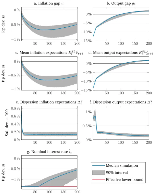
To shed more light on the properties of the model under SL, we look at a specific expectational shock and study how it propagates in the model. This shock can be interpreted as a sudden pessimistic change in the sentiment of households and firms (or negative news), which now expect a recession (Schmitt-Groh´e & Uribe 2017). In our stability graph, this boils down to plotting the transitory dynamics from one specific point of Figure 6 back to the target. Specifically, we simulate a one-time pessimistic shock on output gap expectations of all agents that is large enough to shift the average expectations beyond the boundary of the stability frontier depicted in Figure 6.15 We
can then investigate why and how the system converges back to the target under SL from a point of the state space where it would not under some form of recursive learning. The main outcome of such a shock is a prolonged depressive episode at the ELB (see Fig. 7): inflation and interest rates exhibit considerable persistence below their target while output gap recovers faster, and even temporarily overshoots the steady state. These dynamics entailed under SL are empirically much closer to the recent economic experience discussed in the introduction than the excess volatility in the indeterminacy region under RE or the diverging deflationary paths under adaptive learning.
Let us now unravel the underlying forces at play under SL that deliver those em-pirically appealing dynamics. The initial deviations from steady-state are triggered by the pessimistic shock only, while the resulting prolonged low inflation and ELB envi-ronment stems entirely from the sluggish dynamics of expectations under SL and their self-fulfilling nature in the NK model.
As explained in Section4.1, right after the shock, the most pessimistic forecasts are discarded at the profit of mildly pessimistic but below-target forecasts. This elimina-tion of the most negative forecasts rules out the possibility of deflaelimina-tionary spirals and 15A more realistic approach would be to shock expectations on both output and inflation, but for the purpose of clarity, we limit the analysis to a single shock. In our simulation, agents expect on average a negative output gap of 14% to reach the ELB while keeping inflation forecasts at the target.
50 100 150 200 −1 % −0.5 % 0 % P.p dev . ss a. Inflation gap ˆπt 50 100 150 200 −15 % −10 % −5 % 0 %
b. Output gap ˆyt
50 100 150 200 −1 % −0.5 % 0 % P.p dev . ss
c. Mean inflation expectations ESL t πˆt+1 50 100 150 200 −15 % −10 % −5 % 0 %
d. Mean output expectations ESL t yˆt+1 50 100 150 200 0 % 0.2 % 0.4 % 0.6 % 0.8 % Std. dev .× 100
e. Dispersion inflation expectations ∆π t
50 100 150 200
0 % 0.5 % 1 %
f. Dispersion output expectations ∆y t 50 100 150 200 −1 % −0.5 % 0 % P.p dev . ss
g. Nominal interest rate ˆit
Median simulation 90% interval
Effective lower bound
Notes: From the top left to the bottom right, impulse response functions (IRFs) of inflation gap, output gap, average inflation gap expectations, average output gap expectations, nominal interest rate, standard deviation of individual inflation expectations and standard deviation of individual output gap expectations. The blue plain line represents the median realization, and the dotted lines are the 5% and 95% confidence intervals over 1,000 Monte Carlo simulations. All plots report the zero line. The lower horizontal line on the IRF of ˆıtis the ELB.
Figure 7: Impulse response functions (IRFs) of the estimated model to a one-time −14% output gap expectation shock
generates the ‘missing disinflation’ along the bust. Per their self-fulfilling nature, those mildly pessimistic views nurture the downturn and turn self-confirming, which triggers an accommodating response from the CB given the weight on the inflation gap in the Taylor rule. This stimulating monetary policy has the largest impact on output gap, which eventually turns positive.
The self-fulfilling nature of inflation expectations is exacerbated by the near-unity value of the discount factor and the flat estimated slope of the Phillips curve (see Eq. 2
and remark that the impulse response functions (IRFs) of inflation and the average infla-tion expectainfla-tions almost perfectly overlap). This means that low inflainfla-tion forecasts are almost self-fulfilling and deliver near-zero forecast errors, which allows those pessimistic inflation outlooks to survive and diffuse among the agents.16 This selection mechanism,
together with expectation-driven inflation, explains the considerable persistence in in-flation and inin-flation forecasts depicted inFigure 7. Inflation and inflation expectations cannot converge back on target until the conjugated force of positive output gaps and low interest rates become strong enough to overcome the almost self-fulfilling force of low inflation expectations.17 Those dynamics generate the inflation-less recovery. This prolonged period of positive output gaps may also suggest that the economy may really settle back to equilibrium only after full tapering by the CB.
Finally, it is interesting to note that our model reproduces another stylized fact discussed inMankiw et al.(2003): a recession is associated with an increase in the dis-persion of forecasts among agents or, in other words, the level of disagreement between 16Similar almost self-fulfilling equilibria in the inflation dynamics at the ELB are also reported in Hommes et al.(2019), who use a forecasting laboratory experiment.
17Admittedly, the number of periods before convergence back on target appears implausibly large. However, one should bear in mind that the only policy in our simple model is a Taylor rule constrained by the ELB; hence, our model abstracts from many empirically relevant dimensions of policy that would be likely to play a role in fostering the recovery. The simple structure of the model depicts inflation as almost entirely expectation-driven. It also ignores many other empirically relevant determinants of inflation, for instance investment or wage dynamics, which could also entail a quicker inflation response. Lastly, the shock that we consider is arbitrarily large and is only meant for illustrative purposes, not to match any empirical counterpart in recent history. For these reasons, one should refrain from drawing an explicit time interpretation from those IRFs.
agents.18 Indeed, Figure 7reports how the dispersion of individual expectations spikes in the aftermath of the shock. The rise in forecast dispersion does not last: this is because of the selection pressure of the SL algorithm that pushes the agents to adapt to the ‘New normal’ in the aftermath of the shock. The level of heterogeneity between agents then returns to its long-run value, which is dictated by the size of the mutations. We conclude that our simple model offers a stylized representation of the observed loss of anchorage of long-run inflation expectations depicted in Figure 1 and, more generally, of the inflation dynamics in the wake of the Great Recession and the ensuing recovery as discussed in the introduction. With this model, we offer a reading of this state of affairs as the consequence of the coordination of agents’ expectations on pessimistic outlooks.
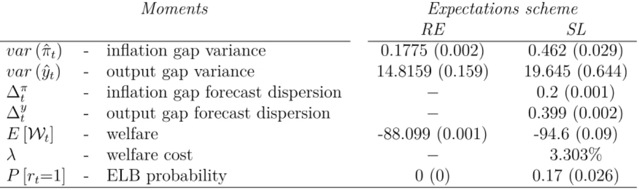
From an allocation perspective, the coordination of expectations on large and per-sistent recessive paths leaves out the economy into second-best equilibria with respect to the benchmark representative agent model under RE.19 Hence, SL expectations can
be envisioned as a friction with respect to the RE representative agent allocation, which may imply a substantial welfare cost, as we now demonstrate.
4.3
Welfare cost of social learning expectations
How costly is the presence of expectation miscoordination in the standard two-equation NK model? To evaluate this cost, we use the welfare function, which has become the main microfounded criterion, to compare alternative policy regimes. Following Wood-ford (2002), we consider a second-order approximation of this criterion and use the unconditional mean to express this criterion in terms of inflation and output volatility. The detailed derivations and explicit forms are deferred to Appendix D. The corre-18In our estimated model, the correlation between output gap and output gap forecast dispersion is significant and reaches -0.34.
19We refer to the RE counterpart of the NK model as the first-best equilibrium because we do not study the welfare implications of the price rigidities vs. the first-best allocation under flexible prices. In this paper, our main focus is the welfare cost induced by expectation-driven cycles.