HAL Id: tel-03181149
https://pastel.archives-ouvertes.fr/tel-03181149
Submitted on 25 Mar 2021
HAL is a multi-disciplinary open access
archive for the deposit and dissemination of
sci-entific research documents, whether they are
pub-lished or not. The documents may come from
teaching and research institutions in France or
abroad, or from public or private research centers.
L’archive ouverte pluridisciplinaire HAL, est
destinée au dépôt et à la diffusion de documents
scientifiques de niveau recherche, publiés ou non,
émanant des établissements d’enseignement et de
recherche français ou étrangers, des laboratoires
publics ou privés.
relational models and expert knowledge
Melanie Munch
To cite this version:
Melanie Munch. Improving uncertain reasoning combining probabilistic relational models and
ex-pert knowledge. General Mathematics [math.GM]. Université Paris-Saclay, 2020. English. �NNT :
2020UPASB011�. �tel-03181149�
Améliorer le raisonnement dans
l’incertain en combinant les
modèles relationnels
probabilistes et la connaissance
experte
Thèse de doctorat de l'université Paris-Saclay
École doctorale n° 581, Agriculture, Alimentation, Biologie,
Environnement et Santé (ABIES)
Spécialité de doctorat: Informatique appliquée
Unité de recherche : Université Paris-Saclay, AgroParisTech, INRAE MIA-Paris, 75005, Paris, France Référent : AgroParisTech
Thèse présentée et soutenue à Paris-Saclay le 17/11 2020, par
Mélanie MUNCH
Composition du Jury
Mme Nacera SEGHOUANI BENNACER
Professeure, CentraleSupélec Présidente
Mme Madalina CROITORU
Professeure des Universités, Université de Montpellier Rapporteur & Examinatrice
M. Manfred JAEGER
Professeur associé, Université d’Aalborg Rapporteur & Examinateur
M. Thomas GUYET
Maître de conférences, l’Institut Agro – Agrocampus Ouest Examinateur
Mme Fatiha SAIS
Professeure des Universités, Université Paris-Saclay Examinatrice
Mme Juliette DIBIE
Professeure, AgroParisTech Directrice de thèse
Mme Cristina MANFREDOTTI
Maître de conférences, AgroParisTech Co-encadrante & Examinatrice
M. Pierre-Henri WUILLEMIN
Maître de conférences, Université Paris VI Co-encadrant & Examinateur
Thèse de
doctorat
: 2020U
PA
SB
011
To my family, that have never quite understood what I was doing, but have always supported me while doing it. Et `a papy, qui aurait fortement appr ´eci ´e l’absence notable de souris dans ce manuscrit. And to grandpa, who would have appreciated the obvious lack of mouses in this manuscript.
ACKNOWLEDGEMENTS
Je n’aurais pu ´ecrire ces lignes sans le soutien de nombreuses personnes, que je souhaiterai re-mercier ici.
Un immense merci donc tout d’abord `a Juliette Dibie, Cristina Manfredotti et Pierre-Henri Wuillemin pour votre pr´esence infaillible, vos conseils avis´es et vos relectures impitoyables. Merci pour votre confiance, pour m’avoir soutenue et autant appris durant ces ann´ees. Merci pour votre exp´erience et vos critiques, qui m’ont permis de m’´epanouir sur un sujet aussi int´eressant. D’un point de vue scientifique comme humain, ce fut un v´eritable plaisir et honneur et travailler `a vos c ˆot´es, que j’esp`ere pouvoir retrouver dans ma vie professionnelle future.
Merci `a l’unit´e MIA-Paris et au laboratoire EKINOCS - anciennement LINK - pour leur ac-cueil dans les locaux d’AgroParisTech. En particulier, je tiens `a remercier Liliane Bel, direc-trice de l’unit´e, et Antoine Cornu´ejols, directeur de l’´equipe, pour leur confiance et support. Merci ´egalement `a Liliana Ibanescu et Christine Martin, sans qui Grignon n’aurait pas ´et´e aussi agr´eable; `a St´ephane Dervaux, qui continue avec d´evotion de manier sarcasmes caustiques et aide pr´ecieuse; `a Joon Kwon, pour ses inestimables explications du dense Causality, de Pearl. Merci `a Erica Helimihaja et Christelle Gehin pour leur patience lors la prise en charge des voyages et des billets d’avion, parfois bien compliqu´es. Enfin, merci `a Pierre-Alexandre, Joe, Sema, Serife, Ir`ene, Martina, Annarosa, Jules et Julie pour ces moments pass´es, qui `a manger des burritos, qui `a boire un chocolat, qui `a donner des conseils en italien, qui `a procrastiner en parlant de tout et de rien; cette th`ese n’aurait pas eu la mˆeme saveur sans vous. Enfin, malgr´e un bref passage entrav´e par une cl´e capricieuse et une pand´emie mondiale, merci au laboratoire LIP6 pour son accueil chaleureux, et pour m’avoir aid´ee `a me faire une place.
Pour leur accompagnement au cours de ces trois ans et tous les perfectionnements qu’elles ont pu apporter, je tiens ´egalement `a remercier V´eronique Delcroix et Nathalie Pernelle pour leur implication dans le comit´e de suivi de th`ese.
Un immense merci `a Manfred Jaeger et Madalina Croitoru, qui ont accept´e d’ˆetre rapporteurs pour cette th`ese. Merci pour vos relectures et conseils. Merci `a eux, et ´egalement `a Thomas Guyet, Fatiha Sais et au Nacera Seghouani Bennacer pour avoir particip´e au jury lors de la soutenance, malgr´e les al´eas de la visio-conf´erence. Merci pour les discussions, vos critiques et remarques qui vont m’aider `a affiner ce travail.
Merci ´egalement aux ´el`eves que j’ai pu voir d´efiler durant ces trois ann´ees, qui m’ont fait prendre conscience du plaisir que l’on peut avoir `a enseigner. Oui, mˆeme avec toi, celui qui a pr´ef´er´e me passer le dictionnaire en string pour faire un .found() en Python plut ˆot que de faire un appel `a dictionnaire comme c’´etait d´ecrit en page 25 du polycopi´e de cours. Je ne t’ai pas oubli´e.
Merci aux organisateurs de la formation doctorale EIR-A d’Agreenium, pour les s´eminaires or-ganis´es, les rencontres effectu´ees et l’opportunit´e offerte de pouvoir effectuer un s´ejour `a l’´etranger.
Merci `a l’´equipe DISI du laboratoire d’informatique de l’universit´e de Trento, pour leur accueil et pour m’avoir permis de d´ecouvrir de nouveaux domaines. En particulier, merci `a Andrea Passerini et Paolo Dragone pour leur encadrement et leur accompagnement tous le long de ces trois mois.
une p´eriode compliqu´ee comme celle de la pand´emie a vraiment ´et´e d’un r´econfort immense. Le travail repr´esente une grosse partie de la vie d’un doctorant. N´eanmoins, celui-ci ne pour-rait jamais ˆetre aussi bien men´e sans le soutien ind´efectible de la famille et des amis autour. Merci `a mes parents, pour leur ´ecoute et leur soutien; `a mes fr`eres et sœurs, et tout ceux qui ont pris le temps de m’envoyer du soutien pendant la th`ese et la soutenance.
Beaucoup d’amis `a remercier ´egalement: Hugo, Arthur, Fabien, Caroline, Franc¸ois, Antoine, R´emi, R´emi, Julien, Laure, Julien, B´er´enice, Chlo´e, Axel... La liste pourrait continuer sur la longueur de la th`ese, et plus encore. Mais je souhaiterai remercier en particulier K´evin, qui a toujours ´et´e l`a quand il s’agissait de m’´ecouter me plaindre, et a toujours su donner les conseils dont j’avais besoin.
Merci `a Paul-Henri, qui a toujours ´et´e l`a, mˆeme lorsque j’´etais `a l’autre bout du monde; qui n’a jamais dout´e, et m’a toujours soutenue.
Et enfin, merci `a Ainu et Arda, dont le talent n’´equivaut pas `a celui de F. D. C. Willard, mais qui ont au moins eu le m´erite d’avoir offert un joyeux divertissement de fin de soutenance.
CONTENTS
Introduction 1
Objectives . . . 4
Thesis Outline and Contribution . . . 6
1 Background and State of the Art 9 1.1 Probabilistic Models . . . 10
1.1.1 Discrete Probability Theory . . . 10
1.1.2 Bayesian Networks . . . 12
1.1.3 Learning Bayesian Networks . . . 14
1.1.4 Essential Graphs . . . 15
1.1.5 Probabilistic Relational Models . . . 17
1.1.6 Learning under constraints . . . 20
1.1.7 Using Ontologies to learn Bayesian networks . . . 21
1.2 Causality . . . 23
1.2.1 Overview . . . 23
1.2.2 Causal discovery . . . 24
1.2.3 Ontologies and Explanation . . . 27
1.3 Conclusion . . . 28
2 Learning a Probabilistic Relational Model from a Specific Ontology 29 2.1 Domain of application . . . 30
2.1.1 Transformation Processes . . . 30
2.1.2 Process and Observation Ontology PO2 . . . . 32
2.2 ON2PRM Algorithm . . . 33
2.2.1 Overview . . . 33
2.2.2 Building the Relational Schema . . . 35
2.2.3 Learning the Relational Model . . . 37
2.3 Evaluation . . . 38
2.3.1 Generation of synthetic data sets . . . 39
2.3.2 Experiments . . . 41
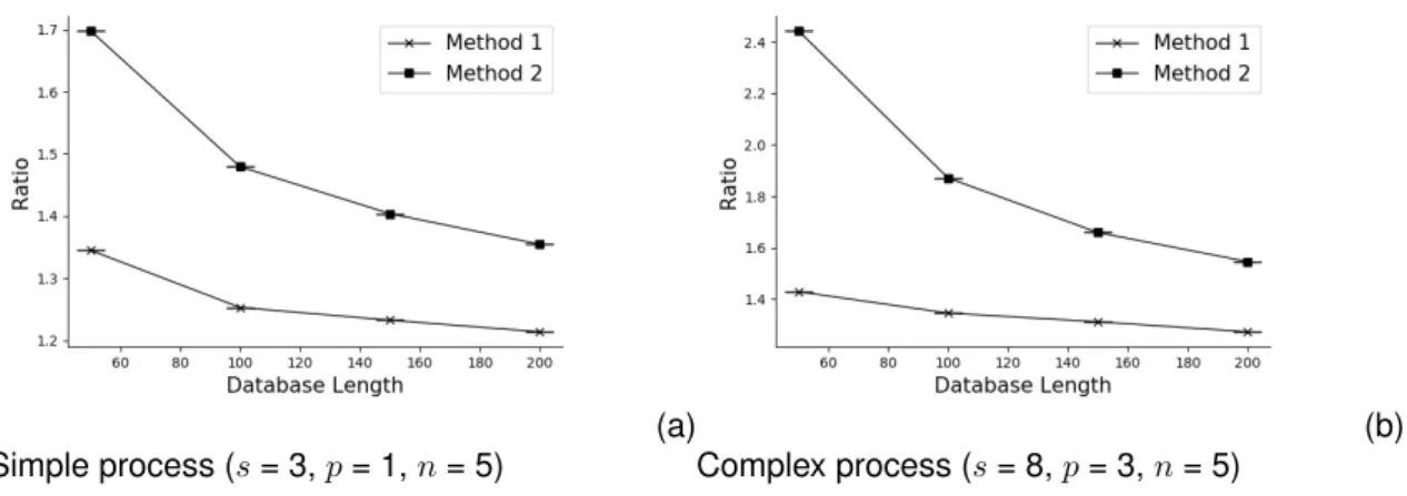
2.3.3 Results . . . 43
2.4 Discussion . . . 46
2.4.1 Determination of explaining and explained attributes . . . 47
2.4.2 Defining the temporality . . . 48
3.1.1 Explicitation of constraints . . . 51
3.1.2 Structure of the Stack Model . . . 53
3.2 CAROLL Algorithm . . . 54
3.2.1 Expert assumption . . . 55
3.2.2 Assumption’s Attributes Identification . . . 57
3.2.3 Enrichment . . . 59
3.2.4 Validation . . . 61
3.3 Towards causal discovery . . . 63
3.3.1 Validating causal arcs . . . 63
3.3.2 Possible conclusions . . . 65
3.3.3 Incompatibility of constraints . . . 66
3.3.4 Discussion . . . 67
3.4 Evaluation . . . 68
3.4.1 Synthetic data set . . . 68
3.4.2 Movies . . . 70
3.4.3 Control parameters in cheese fabrication . . . 72
3.5 Discussion . . . 77
3.6 Conclusion . . . 78
4 Semi-Automatic Building of a Relational Schema from a Knowledge Base 81 4.1 Closing the Open-World Assumption . . . 82
4.1.1 General Idea . . . 82
4.1.2 Defining the Transformation Rules . . . 83
4.1.3 Limits and Conclusion . . . 91
4.2 ACROSS Algorithm . . . 93
4.2.1 Comparison between CAROLL and ACROSS . . . 93
4.2.2 Initialization . . . 95
4.2.3 Relational Schema’s Automatic Generation . . . 96
4.2.4 User modifications . . . 97 4.2.5 Learning . . . 97 4.3 Evaluation . . . 97 4.3.1 Domain . . . 98 4.3.2 Experiments . . . 98 4.3.3 Results . . . 101 4.3.4 Discussion . . . 102 4.4 Final Remarks . . . 104 4.4.1 Limits . . . 104 4.4.2 Expert feedback . . . 105 4.5 Conclusion . . . 105
Conclusion and Perspectives 107 Summary of Results . . . 107
Discussion and Future Works . . . 111
A User’s modifications 115 A.0.1 Delete a class . . . 115
A.0.2 Fuse two classes of the same type . . . 116
A.0.3 Divide a class . . . 116
A.0.4 Create a Mutually Explaining class . . . 117
A.0.5 Remove an attribute . . . 118
A.0.6 Create a relational slot . . . 118
A.0.7 Remove a relational slot . . . 118
A.0.8 Reverse a relational slot . . . 119
1.1 Example of a Bayesian Network using Example 2 . . . 13
1.2 Bayesian Networks’s equivalence . . . 16
1.3 Example of equivalence classes and their associated essential graph . . . 17
1.4 Modeling of a simple process . . . 18
1.5 Structure of a Probabilistic Relational Model . . . 19
1.6 Example of a probabilistic relational model’s system’s instantiation . . . 20
2.1 Example of a transformation process in biology . . . 30
2.2 Example of a transformation process . . . 31
2.3 PO2main schema . . . . 32
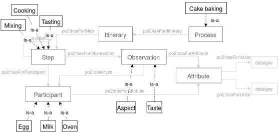
2.4 Example of a domain ontology using PO2 . . . . 33
2.5 Overview of the ON2PRM Algorithm . . . 35
2.6 Generic relational schemaRSP O2. . . 36
2.7 Example of a relational schema built from the domain ontology example . . . 37
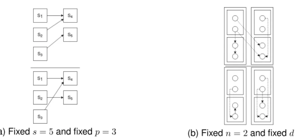
2.8 Variety of the transformation processes structures . . . 41
2.9 Plan of experiments . . . 41
2.10 Evolution of F-score ratio for two different processes with the dataset length . . . . 45
2.11 Evolution of F-score in function of n (p = 1, dataset size = 50) and ratio evolution in function of n and s forM2 . . . 46
3.1 Structure of the Stack ModelRS . . . 53
3.2 Overview of the CAROLL algorithm . . . 54
3.3 Excerpt of a knowledge base about students and universities . . . 55
3.4 Relational schemaRSU built fromHU . . . 59
3.5 Relational schemaRSU built fromHU updated after enrichment . . . 61
3.6 Causal Discovery protocol when a model is learned . . . 64
3.7 Causal Discovery protocol when a model cannot be learned . . . 67
3.8 Example of an instantiated transformation process using the PO2ontology . . . . 69
3.9 Comparison of the different learnings . . . 70
3.10 EG and their relational schema learned during the three iterations . . . 73
3.11 Model constructed from the expert assumptionHc . . . 75
3.12 Summary of the number of observed inter and intra step relations . . . 76
3.13 Excerpt of the EG learned forHc . . . 78
4.1 Small ontology’s example . . . 83
4.2 R0. General case . . . 84
4.3 R1. Missing value . . . 85
4.4 R2. Multiple Instantiations of Object Properties: domain . . . 86
4.5 R3. Multiple Instantiation of Object Properties: multiple range . . . 87
4.7 R5. Distinction between different configurations of multiple object properties: range 90 4.8 R5. Distinction between different configurations of multiple object properties: domain 90
4.9 R6. Self-references in the knowledge base . . . 91
4.10 Overview of the ACROSS algorithm . . . 94
4.11 Examples of cycles in an ontology and how to remove them . . . 96
4.12 Schema of the excerpt of DBPedia used to represent writers . . . 98
4.13 Automatic generation of the author’s relational schema . . . 99
4.14 Relation Schema defined from the knowledge base and the expert’s knowledge . . 101
4.15 Probabilistic relational model learned on a DBPedia extract about authors, and its associated essential graph . . . 102
4.16 Example of a class creation’s user’s modification . . . 103
A.1 Example of a set of instances (a) and its deduced relational schema (b) . . . 116
A.2 Proposition of a division of the Student class . . . 117
A.3 Example of a Mutually Explaining Class . . . 118
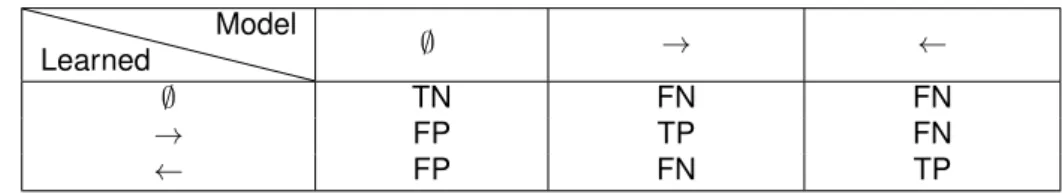
2.1 Heuristic used to compare two BNs . . . 42
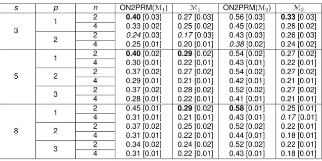
2.2 Variation of the mean F-score in function of different parameters tested with a dataset of size 50 with 100 repetitions . . . 43
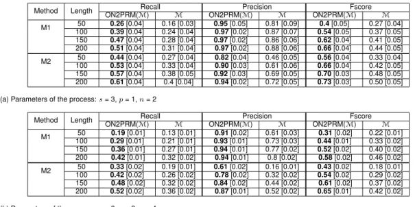
2.3 Comparison of performances for recall, precision and F-score forM1andM2 with different sizes of the dataset . . . 44
3.1 Different cases for causal validation . . . 65
3.2 Discretization of the Movie dataset . . . 71
3.3 Cheese plan of experience . . . 74
4.1 Discretization of the Writers dataset . . . 101
4.2 Joint probability of the attributereleaseDate depending on the attributes writer.birthDate andwriter.min arwu . . . 103
4.3 Summary of the ON2PRM algorithm . . . 108
4.4 Summary of the CAROLL algorithm . . . 109
4.5 Summary of the ACROSS algorithm . . . 111
‘I’m sure. But look at it this way. What really is the point of trying to teach anything to anybody?’ This question seemed to provoke a murmur of sympathetic approval from up and down the table. Richard continued. ‘What I mean is that if you really want to understand something, the best way is to try and explain it to someone else. That forces you to sort it out in your own mind. And the more slow and dim-witted your pupil, the more you have to break things down into more and more simple ideas. And that’s really the essence of programming. By the time you’ve sorted out a complicated idea into little steps that even a stupid machine can deal with, you’ve certainly learned something about it yourself. The teacher usually learns more than the pupil. Isn’t that true?’
The idea of an artificial intelligence (AI) able to define concepts and reasoning with them has al-ways been an appealing idea, even at the earliest beginning of computer science. Widely consid-ered as the first computer programmer, Ada Lovelace acknowledged in 1843 in her notes describ-ing the first algorithm in history (dedicated to compute Bernoulli numbers) that the true potential of computers was their ability to deal with abstract concepts (Menabrea et al., 1843) rather than just being number crunchers. Although she also conceded that at that time machines were only capable of computation and not creation, the concept of an AI able to apprehend and mimic com-plex human reasoning kept being brought back, in particular by Alan Turing who even designed a test to evaluate the potential of such an AI (the famous Turing test, still never succeeded to this day) (Turing, 1950).
In the mid 1970s the field of expert systems emerged with the goal of mimicking the deci-sion making process of a human, usually narrowed to a specific domain, such as medicine with MYCIN (van Melle, 1978), an expert system dedicated to diagnose infectious diseases, or che-mistry with DENDRAL (Buchanan and Sutherland, 1968), able to infer molecules structure from spectroscopic analyses. Expert systems are based on the transcription of expert rules (such as: ”If a customer buys a car, then they might be interested in an insurance”) into logical predicates that allow logical and probabilistic inferences. Expert systems are divided into two distinct parts: the knowledge base, that encompasses all the facts and rules the system needs to know; and the in-ference engine, that combines the rules of the known facts to infer new truths. If at the beginning the knowledge bases were fairly small, they quickly grew in size with time. As a consequence the problem of their structuring was raised, and how it should be dealt with in order to ease the ”human to computer” translation. This gave room to knowledge engineering, term coined by Freigenbaum(Feigenbaum and McCorduck, 1983), a key contributor to DENDRAL. The main
idea behind this new domain was to give tools to build, maintain and interact with resources previously defined by human operators. The aspect of knowledge representation was here a key feature, to which ontologies brought an answer.
In the 1980s ontologies were considered in AI both as a philosophical concept to describe the world, and as a component for knowledge-based systems. The first use of the term in the way we now know it can be traced to Tom Gruber, who laid the foundations of their current definition. In his work, he defines ontologies as a group of domain’s concepts and relations that can be used to describe any agent or community of agents (Gruber, 1995). Indeed, ontologies organize and structure the knowledge in terms of concepts, relations between them, and instances (Staab and Studer, 2009). According to Feilmayr and W ¨oß, ontologies’ success stems from this huge adaptability: ”An ontology is a formal, explicit specification of a shared conceptualization that is characterized by high semantic expressiveness required for increased complexity.”(Feilmayr and W ¨oß, 2016). This adaptability allows them to be defined on different levels depending on their genericity (Guarino, 1998). In this thesis, we will focus on domain ontologies, which are used as a common and standardized vocabulary for representing any domain (e.g. life-science, geogra-phy). Those ontologies can be defined using different reference languages as recommended by the W3C1. In the following, we will consider only the RDF2 and OWL3 languages, which are based on the XML markup language.
RDFis a formal representation model for resources where data is written as <subject, predi-cate, object> triple. Subject and predicate are denoted by a unique Universal Ressource Identifier (URI); in the case of the object, it can also be a unique URI, or a datatype (such as a number, a name, etc.), depending of the relation we want to describe. For instance:
• <db:International Semantic Web Conference, dct:subject,dbc:Artificial intelligence con-ferences>4identifies the subject of the International Semantic Web Conference (ISWC) as the AI, which is also another resource of this website, with other predicates.
• <db:International Semantic Web Conference, dbp:history, ”2002”>, on the contrary, states that the ISWC has been created in 2002, which is strictly a value.
OWLhelps to extend the RDF notation by adding the concepts of classes, properties and axioms, which provide more semantic. In this thesis, we will mainly use the concepts of:
• Class: a class represents a entity such as a conference, a movie, an animal... Semantically it
1World Wide Web Consortium, who promotes standards for every web-related developments: http://www.w3.org/XML
2https://www.w3.org/RDF/
3https://www.w3.org/OWL/
4For a better readability those URI have been shortened using a prefix. db stands for http://dbpedia.org/page/, dct for
https://dublincore.org/specifications/dublin-core/dcmi-terms/subject#, dbc for http://dbpedia.org/page/Category and dbp for http://dbpedia.org/page/property
embodies the same entity (e.g. a lion) that can then be instantiated multiple times. Example: zoo 1, which is an instance of the class Zoo, has three lions, instances of the class Lion: lion 1, lion 2 and lion 3.
• Object Property: an object property is a relation that links two classes or instances, with one as the subject (the domain) and one as the object (the range). This relation is written as a triple. Example: the property hasForAnimal helps to define the animals of a zoo: <zoo 1, hasForAnimal, lion 1>. A symmetric property can also exist: <lion 1, isAnimalOf, zoo 1>. • Datatype Property: a datatype property is a relation that links a class or an instance to a
data value. The individual and the data are always respectively the subject and the object. Example: the property hasForAge attributes an age to each animal, for instance <lion 1, hasForAge, ”15”>. Since the object is always a data value, there is no symmetric property for the datatype properties.
Thanks to the introduction of ontologies, domains can now easily be structured. However, the more complex they grow, the more difficult their data’s analysis also becomes. Indeed, adding more facts opens to more issues, such as incomplete data, which renders analysing more chal-lenging since information is missing. In addition to this, there is intrinsic uncertainty in many complex domains, as the observed phenomena are not always fixed and cannot be determined with certainty.
Example 1. An omniscient robot would be able to give an accurate weather estimate of to-morrow, as it would know every relevant parameters to compute its prediction. A common human, however, would only have access for instance to the sky; the only prediction they would be able to give would be of the form ”If the sky is cloudy, then rain is highly probable”.
All of these new issues add subtleties that need specific tools in order to study and analyze them. Since ontologies and classical system experts are dedicated to logical reasoning, other va-rious approaches have been proposed to expand their ability to work with such complex domains, such as for instance probabilistic reasoning which is best suited for dealing with uncertainty. Frameworks have already been proposed:
• BayesOWL (Ding et al., 2006, Zhang et al., 2009) and a similar framework OntoBayes (Yi Yang and Calmet, 2005) directly represent a probabilistic model using the OWL notation. • MEBN/PR-OWL and PR-OWL 2.0 (Carvalho et al., 2013, da Costa et al., 2008) represents
in a similar fashion a probabilistic model using PR-OWL 2, an upper ontology written in OWL.
continuous and discrete data in an ontology (on the contrary of the previous frameworks that were only able to deal with discrete variables).
These frameworks represent an interesting and efficient way of modeling the probabilistic dependencies, while offering a way for using probabilistic inference tools within the ontology. However they do not offer a way to learn such dependencies between the different values of the ontology.
In this thesis, we present novel methods in order to bridge this gap between ontological knowledge and probabilistic reasoning. Our work will present and develop different methods to exploit and reason on the knowledge encapsulated in knowledge bases using probabilistic learning.
OBJECTIVES
Reasoning over a domain requires to have the objects of interest modeled, usually through the means of different variables. In Example 1, for instance, the weather can be represented by the rain frequency, the clouds opacity, etc. Therefore, a good modeling of such a domain requires to represent these variables. However, if we want this model to be explanatory, we need to repre-sent the probabilistic dependencies between these variables. To do that, the scientific method for instance rests on several well-defined steps, with among them formulating and verifying hypo-thesis through experiments. Experiments, however, are sometimes difficult to carry out, for legal, practical, temporal, economical or ethical reasons: to this intent a model can help amplify the human thought process (Churchman, 1968), and give scientists a better overview on the whole operation. As a consequence, modeling is a large part of the scientific method: it helps to encom-pass all known facts, to reason with them as a whole set, and to check the formulated hypothesis for making predictions.
Yet learning an accurate modeling of any given domain can also be a hard problem, which nearly every time requires a good grasp of its issues. Indeed, the choice of the model basis and its key components is essential and, if done wrongly, can throw off the whole model’s predictions. For instance in statistical models, the most critical part of the analysis usually depends of the quality of the translation from the core subject to the model (Cox, 2006).
In this thesis, we offer new methods to use knowledge about domains encompassed in know-ledges basesin order to improve probabilistic reasoning. The term ”Knowledge base” is often used interchangeably in literature with other such as ”ontologies” or ”knowledge graphs” (Ehrlinger and W ¨oß, 2016). Since Google introduced this last term in 2012 to refer to the use of semantic knowledge in Web search, no concrete definition has been given. Several attempts have been
made on the requirements a knowledge graph should have, based on characteristics such as the size (Huang et al., 2017), or on the restriction only to RDFs bases (F¨arber et al., 2017). In this dissertation, we will consider the definition of Ehrlinger and W ¨oß (2016) in which a knowledge base is an ontology structure combined with a large population. More formally, we denote a knowledge base KB as a couple (O, F) where the ontology O is represented in OWL and the knowledge graph F represents the data in RDF.
• The ontology O = (C, DP, OP, A) is defined by a set of classes C, a set of owl:DatatypePro-perty DP inC × TDwith TDbeing a set of primitive datatypes (e.g. integer, string), a set of owl:ObjectProperty OP inC × C, and a set of axioms A (e.g. property’s domains and ranges).
• The knowledge graph F is a collection of triples (s, p, o), called instances, where s is the subject of the triple, p a property that belongs to DP ∪ OP and o the object of the triple. Our main goal is to learn a probabilistic model in order to discover new knowledge using the F triples and the semantic information brought by O.We chose to focus on specific domains that shared common features such as uncertainty, missing values, complex relations between the potential variables that were possible to model using probabilistic models. Probabilistic models are dedicated to represent random variables and the relations between them under the form of probabilistic distributions (that we will detail in Chapter 1). This allows (1) a good flexibility, as all domains with uncertainty can be represented and (2) a good readability. Indeed, on the contrary of some ”black-box” models such as the neural networks, that present a very efficient way to learn but a poor explainability of the learned results, probabilistic models allow the analysis of the relations between the variables. This usually gives a visual and interpretable model, useful when dealing with complex domains.
In this thesis we present and develop three different methods for guiding the learning of a probabilistic model using expert knowledge. The novelty of our approach is that this expert knowledge is brought from the knowledge base on one hand, and from a human expert of the domain on the other hand, which guaranties a model learned as close as possible to the target domain. Moreover, throughout our work, one of our main goals was the accessibility for the so-called experts. This accessibility is expressed on two levels: (1) during the extraction of the on-tological knowledge used for the learning, and (2) for the learned model exploitation afterwards. For all our contributions the focus has been set notably on causality as part of causal discovery, which is an hard but rewarding goal when it comes to modeling and understanding complex domains.
different paradigms. Both are dedicated to describe a model as close as possible to the reality, but with two different visions: while the Bayesian approach favors the statistical analysis of the given data in order to discover knowledge among what it already knows, the ontological approach is based more on the information brought by the expert in order to discover new explicative and predictive rules. In these thesis however we will demonstrate how both of these approaches can mutually benefit by 1) enhancing the reasoning with probabilistic variables by introducing semantic knowledge and 2) enriching the ontological knowledge by learning new rules.
THESISOUTLINE ANDCONTRIBUTION
This thesis is organized in several chapters. All of the original works are validated and illustrated with complete examples that were used to validate our publications.
• Chapter 1. Background and State of the art gives an overview on the different methods we used and the state of the art. It focuses on probabilistic models such as Bayesian networks (BNs) and Probabilistic Relational Model (PRMs), as well as their learning, especially under constraints. A second part of this chapter is dedicated to causality, causal discovery, and the main challenges they raise.
• Chapter 2. Learning a Probabilistic Relational Model from a specific ontology presents an example drawn from a given ontology, and how it can be used to learn a probabilistic model. In this chapter, we focus on how using an ontology can greatly help to learn a model closer to the reality. We introduce here our first contribution, the ON2PRM algorithm, which allows to learn a probabilistic relational model from any domain ontology using the specific core ontology presented in this chapter.
Publications.
– Munch M., Wuillemin PH., Manfredotti C., Dibie J. and Dervaux S. Learning Proba-bilistic Relational Models using an Ontology of Transformation Processes. In: ODBASE 2017.
• Chapter 3. Interactive learning from any knowledge base presents CAROLL, a first algo-rithm dedicated to build a relational schema from any knowledge base by using a human expert contribution. This method is guided by a causal assumption formulated by the ex-pert. The aim of the causal assumption here is to motivate the learning of the model by giving it a precise purpose: checking whether the expert’s belief is true or not. In this chap-ter, we present this method as well as the causal discovery aspect of our work.
Publications.
E. Identifying control Parameters in Cheese Fabrication Process Using Precedence Con-straints. In: DS 2018.
– Munch M., Dibie J., Wuillemin PH. and Manfredotti C. Towards Interactive Causal Relation Discovery Driven by an Ontology In: FLAIRS 2019.
• Chapter 4. Semi-automatic learning from any knowledge base presents ACROSS, an al-gorithm where the contribution required from the expert is reduced compared to the algo-rithm introduced in the previous chapter. Our aim here is to be able to learn a probabilistic model from any knowledge base while easing as much as possible the workload asked to the expert. In this chapter we give a detailed overview of the differences with the previous methods, as well as the tools given to the expert in order to help them.
Publications.
– Munch M., Dibie J., Wuillemin PH. and Manfredotti C. Interactive Causal Discovery in Knowledge Graphs. In: PROFILES/SEMEX@ISWC 2019.
• Conclusion and Perspectives summarizes the results presented in these thesis, discuss their limitations and presents some perspectives works for the future.
Domain studied in this thesis
Several in-use knowledge bases will be presented in this thesis, reflecting the adaptability of our methods. One uses the Process and Observation Ontologya(PO2), dedicated to trans-formation process; and two have been extracted from DBPediab, restricted to the subjects we wanted to analyze. The first is about moviescand have been enriched with information from the website ImDBd. The second is about books’ authorse.
ahttp://agroportal.lirmm.fr/ontologies/PO2
bhttps://wiki.dbpedia.org/
chttps://bit.ly/2RYVjG8
dhttp://www.imdb.com/
BACKGROUND AND STATE OF THE ART
The main challenge of our approach is the combination of two different domains of artificial intel-ligence that are not usually studied together: knowledge representation and uncertainty reason-ing. We already have briefly presented, in the introduction, knowledge bases and how we define them in this thesis. In order to better understand the issues and challenges raised, this chapter presents the state of the art on the different tools we have used.
Section 1.1describes probabilistic theory (1.1.1), and more especially Bayesian networks (1.1.2), how to learn them (1.1.3), and essential graphs (1.1.4). In subsection 1.1.5, we present a Bayesian networks’ object-oriented extension: the probabilistic relational models. The goal of this thesis is to propose an approach combining ontologies and probabilistic models in order to learn a model semantically close to the reality. As a consequence we do not offer an extended comparison be-tween the different learning methods, as it falls out of the scope of our study. That is why in these sections we only briefly touch the learning algorithms and scores chosen for the rest of our work; but since learning using ontology knowledge is similar to learning under constraints, we develop the current state of the art on the matter (1.1.6). The last section is dedicated to explain the works aiming to combine probabilistic models and ontologies (1.1.7).
Section 1.2presents the main ideas we develop in this thesis on the matter of causality. It first covers the principal definitions and tools described in the literature (2.2.1) that we use in this thesis. Afterwards it presents the problem of causal discovery (1.2.2) and how it is handled in other works. It concludes with some thoughts on causality, ontologies and explanation (1.2.3).
1.1 PROBABILISTICMODELS
Probabilistic models are an efficient way to express probabilistic dependencies between different variables. They fall into different categories, depending on the way these relations are expressed. In these thesis, we will concentrate on probabilistic graphical models which use graph theory to show the conditional dependence structures. In order to introduce these models, we first give a short review on discrete probability theory.
1.1.1 DISCRETEPROBABILITYTHEORY
We define a random variable as a variable that can present different states. For each problem we wish to study, we define a set of variables able to describe all of its parameters.
Example 2. We define three random Boolean variables R, S and G. These respectively ac-counts for whether it is raining (True) or not, whether the sprinkler is on (True) or not, and whether the grass is wet (True) or not. Our problem is then described by the Cartesian prod-uct of all the possible values for each variable: { (R,S,G), (¬R,S,G), (¬R, ¬S,G)...}.
The goal of discrete probability theory is (1) to evaluate, for each of the defined variables, the mapped probability function; and (2) to express, if possible, the impact of a group of variables over the others. To do so, we denote X as a random variable, and P (X) its associated law.
Using it, discrete probability theory aims to answer two kinds of questions:
1. ”What is the probability that X takes the value xi and Y the value yi?”, which is denoted P (X = xi, Y = yi). P (X, Y ) is known as the joint probability.
2. ”What is the probability that X takes the value xiknowing that Y has taken the value yi?”, which is denoted P (X = xi|Y = yi). P (X|Y ) is known as the conditional probability and is read ”probability of X knowing Y ”. It is important to note that this probability is defined only if we deal with a non-zero intersection, i.e. P (Y = yj) > 0.
Independence
In the particular case where X and Y are independent (meaning the value of one has no influence over the value of the other), those quantities can easily be computed, with:
1. P (X = xi, Y = yi) = P (X = xi)P (Y = yi) 2. P (X = xi|Y = yi) = P (X = xi)
We distinguish discrete from continuous probability theory with the types of random variables used to describe the problem. Indeed, if the number of variable’s states is finite or countable, then
we consider the variable as discrete, meaning all of its states can be singled out. On the contrary, if the states are represented by the set of real numbers R (or a portion of it), then the variable is considered as continuous.
Example 3. When we consider a coin throw, the space is usually finite, with each state re-ferring to a possible outcome: Dcoin = {head, tail}. On another hand, when we consider the average income of a population, we deal with quantities that cannot realistically be listed, thus: Dincome= R+. If we want to study it with the discrete probability theory, we thus have to discretize its values, by creating categories in which every possible value can be sorted.
Determining (X1, X2, ...Xn)
Defining a space sometimes requires to discretize all the possible outcomes, event the less likely.
The discretization occurs when we want to specify different categories among those we are presented with. In this thesis, the most usual case is when we have a continuous space that we want to transform into a discrete one: for instance, Dincome = R+ can become Dincome = {D<1200, D>1200} where we distinguish between when the income is less than 1200 and when it is bigger.
If we consider a coin’s tossing, a lot more is theoretically possible than just head or tail: the coin can fall on its edge, or be lost, or stolen,... We however chose to consider that the coin will always fall back either on head or tail, and ruled out these other possibilities.
In this thesis, we will only briefly cover this subject, as it is not at the core of our work. It is however essential to keep in mind that defining the different states we will take into account in our problem is already taking a stance in the modeling of our event
Both discrete and continuous variables have different properties and definitions; in the fol-lowing we will only consider the discrete probability theory. This implies that all the variables we deal with are either (1) discrete or (2) have been discretized. Discrete probability theory at-tributes to each variable’s state a probability that varies between 0 (the state will never occur) and 1 (the state is certain); the probability of the union of all the possible states is 1, meaning the space represents indeed all of the possible values. For the following, we denote P (x) the marginal probabilityrepresenting P (X = x).
Example 4. If in our coin example the coin is balanced (meaning one side is not favored over the other), then we have P (tail) = P (head) = 0.5: no event is more likely to happen than the other. Moreover, P (tail) + P (head) = 1, meaning that we do not take into account other
outcomes.
In a more general setting, we can express the rule of the marginal probabilities sum and the rule of the probabilities product. Be DomainV the set of all possible values of the random variable V, we have
Property 1. ∀x ∈ DomainX, ∀y ∈ DomainY, P (x, y) = P (x|y)P (y) = P (y|x)P (x) It can be written as P (X, Y ) = P (X|Y )P (Y ).
Property 2. P (x) =P
y∈DomainY P (x|y)P (y).
It can be written as P (X) =P
Y P (X|Y )P (Y ).
Using Property 1, Thomas Bayes defined in 1763 his famous Bayes’ rule (Bayes, 1763). Theorem 1: Bayes’ rule. Being X and Y two random variables such that P (Y ) 6= 0, we have
P (X|Y ) =P (Y |X)P (X) P (Y )
This theorem helps to express the a posteriori probability of X, meaning the probability of X after Y has been observed. This is especially useful as it helps to compute any probability, given we know (1) its conditional probabilities and (2) the marginal laws a priori. We can also express Bayes’ rule as P (X|Y ) ∝ P (Y |X)P (X), meaning that P (X|Y ) (the posteriori) is proportional to the product of P (Y |X) (the likelihood) and P (X) (the a priori). Following this intuition, Pearl (1988) presented a probabilistic graphical model based on Bayes’ rule, the Bayesian network.
1.1.2 BAYESIANNETWORKS
A Bayesian network is a probabilistic graphical model based on the representation of different variables and their influence on each other using tools from the graph theory.
Definition 1: Bayesian Network. A Bayesian Network of dimension n is defined by:
• a directed acyclic graph G = (V,E), where V and E are respectively the set of all its nodes and arcs. V contains n nodes, each representing a variable. For simplification’s purpose, we associate in the following the variables with their graphical representation (i.e. their representing nodes).
• a set of random variables equal to V and defined such that:
p(V ) = Y x∈V
p(x|P arents(x))
Since the value of a variable depends only on the values of its parents (i.e. the parents of the associated node in the graph), then a Bayesian network is the graphical representation of the dependencies between the variables. To each node with parents, a conditional probability table is assigned, which gives the probability values of each value of the variable in function of the value of its parents variables.
Figure 1.1: Example of a Bayesian Network using Example 2.Each variable has a conditional prob-ability table that shows how their values depend on their parents.
This allows a double reading very useful for our analysis. Suppose we want to model the system described in Example 2, and that we have learned the Bayesian network presented in Fig.1.1. We can then easily answer two types of questions:
• Qualitative questions: ”Does the value of the grass variable depend on the value of the rain varia-ble?” A simple look at the graph can answer: since there is an arc from the Rain node to the Grass node, then we can deduce they are not independent. We can also see that the Rain is not the only variable with an influence over the Grass, since Sprinkler and Grass also share an arc.
• Quantitative questions: ”What is the influence of the rain variable over the value of the sprinkler variable?” We can then look at the conditional probabilities table and answer: for instance, if we have Rain=True, then the probability that the Sprinkler is actually On is 0.1, which is low. However, if in this example the answer can appear as trivial (since a simple look at the graph could help answer it), these kind of questions can become much harder when involving non-direct relations (such as: ”What is the influence of the rain variable over the value of the grass variable?”).
In order to allow this double analysis, we first need to learn the Bayesian network. It requires two steps: a first for learning the structure of the graph, and a second to learn the probabilistic parameters.
1.1.3 LEARNINGBAYESIANNETWORKS
Learning a Bayesian network’s structure is a NP-hard problem (Chickering et al., 2002), since as the number of variables goes up, the number of possible structures also raises: a 10 variables problem has for instance approximately 4.1018 possible solutions. As a consequence, the most common way to efficiently learn a structure is to look for graphs subsets in order to eliminate the least effective solutions and avoid considerable amount of useless calculations. There are two principal manners for selecting these structures: independence (or constraints) based algorithms, and score based algorithms .
• Constraints based algorithms (e.g. PC Spirtes et al. (2000)) are based on statistical tests. They are structured in three steps. Firstly, a non-oriented graph is built using independence tests between the variables. Then, once the first graph has been built, other independence tests are used to single out the specific structure A → B ← C, also called V-structure. Indeed, V-structures indicate a complete independence between A and C, which can help orient the edges (an example on a possible use of V-structures to orient edges is given in Example 19). Finally, once all V-structures have been identified, the rest of the edges are also oriented, being careful not to create V-structures.
• Score based algorithms, on the contrary, are composed of two parts: a search algorithm (e.g. Greedy Equivalent Search GES Chickering (2003)) and an heuristic score (e.g. AIC (Akaike, 1974), BIC (Schwarz, 1978) or BDeu (Buntine, 1991)). At each iteration of the algorithm, a change is brought to the graph (addition, removal, inversion of an arc) and a new score is computed. Scores are composed of two parts: firstly, they tend to search for the best structure that maximizes it. However, this component alone is not good enough, as it tends to favor complete graphs (i.e. graphs where each node are linked to the others), which usually result from over-fitting. As a consequence, scores also have to take into account a simplification factor, which applies Occam’s razor philosophy: the simplest solution is usually the best.
From an historic point of view, constraint based algorithms (such as PC) learning results have been considered as better than score-based ones, due to the use of statistical tests. Moreover, in the scope of causal analysis theory that have been defined over the past years, these methods are also better than the score based algorithms. Yet, the statistical tests constitute also one of their weaknesses, as they can become quickly very demanding of data in order for their predictions to be robust. That is why score based algorithms are in the end usually more used than constraint based.
The main idea of our work is to integrate ontological knowledge as a constraint into the lear-ning. However, the way classical constraint based algorithms are defined do not allow knowledge other than the one deduced from independence tests. In particular, even if we try to integrate our own semantic constraints, conflicts can be raised if they contradict what the algorithm have determined (e.g. two variables are statiscally dependent but the ontology tells us that they are not). As a consequence, we chose to use an heuristic algorithm, as they were the most efficient solution for integrating constraints from ontological and expert knowledge.
Once a structure has been found the probabilistic dependencies can be learn. To do so, two methods are also possible: a statistical learning based on the maximization of likelihood, or a Bayesian learning based on the estimation of the parameters considering the data set as ad-ditional unobserved variables. This last method, however, is very demanding and expensive, making the first solution easier to use. The learning of parameters consists thus in estimating P (X|parents(X))in the dataset. This is mainly done by estimation of the frequencies and the consideration of a priori (Koller and Friedman, 2009).
One of the drawbacks of this approach is that when the scores are very close a structure can be chosen over another although both are valid choices. In particular, this can be highly critical when it comes to arc orientation. As stated before, the orientation of an arc in the Bayesian network only shows that one variable’s values depend on another variable’s values, given the computed probability tables. However, whether the orientation would be A → B or A ← B is usually not significant, as the marginal probabilities P (A) and P (B) are the same: those structures are said to be part of the same Markov equivalence’s class.
Method used
For the rest of this thesis, unless otherwise stated, we learn Bayesian networks using a Greedy Hill Climbing algorithm with the BIC score.
1.1.4 ESSENTIALGRAPHS
Learning a Bayesian network requires two steps: learning the structure, and then learning the probabilistic parameters from data on that structure. However, even if two structures are diffe-rent, they can sometimes lead to the same joint distributions, as shown in Fig.??.
On the contrary, some arcs’ orientation cannot be reversed without modifying the probabilistic dependencies. This is the case when they indicate independence between the nodes.
Figure 1.2: Bayesian Networks’s equivalence.In this example, BN1and BN2have a different structure but lead to the very same joint distributions. They are said to belong to the same Markov equivalence’s class.
Example 5. Given three variables A, B, C, a structure such as A → B ← C indicates an inde-pendence between A and B: fixing one (i.e. imposing its value) can give information about the other, but will have no impact on it. This particular configuration is called a V-structure, and its arc’s orientation cannot be reversed without changing the nodes’ independences: if we reverse A → B or B ← C, then A and B are no more independent.
Definition 2: Immorality. An immorality is a V-structure A → B ← C where there is no path linking A and C.
An essential graph (Madigan et al., 1996) is a semi-oriented graph designed to represent im-moralities in graphs. Every Bayesian network has one, with which it shares the same skeleton (i.e. the same graph structure but non-oriented). It has two kind of edges:
• Oriented arcs which designate all the Bayesian networks’ arcs that are oriented the same way. Indeed, if all the models that have the same equivalence class have an arc oriented the same way, then this orientation is kept in the essential graph.
• Non-oriented arcs which, on the contrary, designate Bayesian networks’ arcs that can be reversed without modifying the probabilistic dependencies. They are called non-essential arcs.
Two different Bayesian networks can share the same essential graph. In this case, they are said to be part of the same Markov equivalence’s class. Essential Graphs are used to find arcs’ orienta-tion that are dependent of the learning: if an arc is oriented in the essential graph, then it means that no matter the learning, it will always be that way. They are not causal by essence, but under the right hypothesis (that we will detail later), they can be used to deduce causal knowledge.
Figure 1.3: Example of equivalence classes and their associated essential graph. (a) In this ex-ample, due to the V-structure, there is only one Bayesian network in the equivalence class, which thus has the same structure as the essential graph. (b) In this example, the equivalence class is composed of three Bayesian networks. Since none of the arcs are oriented the same way in the three examples, the essential graph is only composed of edges. (c) In this example, the equivalence class is composed of two Bayesian networks sharing a V-structure. The resulting essential graph is composed here of oriented and non-oriented edges.
1.1.5 PROBABILISTICRELATIONALMODELS
Bayesian networks are useful to represent probabilistic dependencies between a set of nodes. Their learning only requires a database composed of distinct examples with all the variables and their values. However, they can be limited when presented with complex settings with multiple nodes as they make no distinction between those during the learning. This is the case whenever one wants to learn a probabilistic model where a same group of nodes is repeated multiple times (see Example 6 for a detailed example). Since the Bayesian network cannot make distinctions, then this group has to be learned as many times as it is present, which increases the error margin.
Example 6. Be a process requiring the use of an oven for multiple steps. This oven is rep-resented by three attributes: the temperature T e, the time T i and the energy E. The higher and longer the temperature and time are, the higher the consumed energy is: the probabilistic relation is T e → E ← T i. Since the oven is used at multiple steps during the process, then we have multiple measurements for the oven’s attributes, one for each use, that we denote StepN.Xfor ”attribute X measured at Step N”. As a consequence the learning set is composed of multiple instances of the same attributes measured at different times, as shown in Fig.1.4. Our goal would be to learn T e → E ← T i; however, this is not possible, as the learning makes no link between Stepi.Xand Stepj.X, which are considered as two different attributes.
More-over, attachment to a class is not taken into account: Stepiand Stepjare not considered as two different entities. As a consequence, in the best case scenario, we would only be able to learn two small networks Step1.T e → Step1.E ← Step1.T iand StepN.T e → StepN.E ← StepN.T i, instead of the only one we would like to learn.
Figure 1.4: Modeling of a simple process.If we want to model a process using multiple times an oven represented by three attributes T e, T i and E, then the database used for the Bayesian network will have multiple instances of these attributes with no way of distinguish them as ”part of the same entity”.
This is particularly restraining for the modeling of complex domains described by ontologies, where a same class can be instantiated multiple times. Ideally, we would like our learning to take into account the structuring brought by the ontology, where each concept is represented by an OWL class that can be instantiated one or multiple times. Considering this would require the learning to be able to comprehend:
• Object properties. They organize the relations between the classes that should be exploited. For instance, a isBefore object property creates a temporal property between two classes. Given two instants ti and tj such that ti < tj, an attribute from ti can be parent of an attribute from tj, but not the contrary (since we want to learn an explanatory model the future cannot have an influence on the past).
• Classes instantiations. If a same concept (i.e. an apparel, a person, ...) intervenes multiple times in our domain, we would like to learn a single model to represent it, and not one model for each instance of this concept. This is the case developed in Example 6.
This cannot easily be done with a classical Bayesian network, and that is why in this thesis we propose to couple ontologies with an oriented-object extension of Bayesian networks called probabilistic relational models.
Probabilistic relational models have been first proposed by Friedman et al. (1999). They en-compass multiple relations between class-object Bayesian networks, thus allowing a better repre-sentation between the different attributes (Torti et al., 2010). To allow such complexity they are defined on two levels (whereas Bayesian networks only requires one): the relational schema and
the relational model.
• The Relational Schema (Fig.1.5(a)) defines different groups of attributes called classes. Classes can be referenced to each other through so-called reference slots. The relations between classes are represented by oriented relations going from a class towards another, and are called slot chains (as they use reference slots to be defined). The orientation of these relations is important, as it will have an influence on the learning of the Relational Model: it is always unique (two classes cannot mutually refer to each other). At this point, only the group of attributes are defined and not the probabilistic dependencies.
• The Relational Model (Fig.1.5(b)) defines the probabilistic dependencies between the at-tributes. While the intra-classes relations are not constrained (in our example, relations between {X, Y } or between {U , V , W }, meaning that inside these sets any probabilistic relation can be learned), the inter-classes’ probabilistic dependencies are influenced by the slot chains: (1) if there is no slot chain between two classes, then their attributes cannot share probabilistic dependencies; (2) if there is one, then the direction of the probabilistic dependencies must follow the orientation of the slot chain.
Ontological and Relational Schema’s classes
The term class is used both for the ontology and the relational schema indifferently. Howe-ver, the distinction is important, especially in our work where they are used for different purposes. That is why, for the rest of this thesis, we distinguish them by annotating ontolo-gy’s classes as O-classes.
Figure 1.5: Structure of a Probabilistic Relational Model. A Probabilistic Relational Model is de-scribed by two levels. (a) The relational schema defines groups of attributes as classes, and how those are related. (b) The relational model gives the probabilistic dependencies between the attributes.
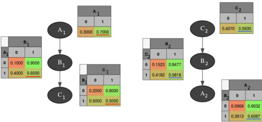
Once both the relational schema and model are defined, the classes can be instantiated to build a probabilistic system. Using classes A and B defined in Fig.1.5, we can build a system as a combination of classes with respect to the reference constraints defined in the relational schema. Once defined, it can be instantiated as shown in the example presented in Fig.1.6. An
instancia-ted system is considered as a classical Bayesian network: therefore it shares the same properties presented in this section, and has an essential graph.
Figure 1.6: Example of a probabilistic relational model’s system’s instantiation.Using the classes defined in Fig.1.5 we can instantiate this system, composed of two classes A and three classes B.
Learning a probabilistic relational model can be an hard task, as one should both learn the relational schema and model. In this thesis, we focus on two parts:
• The translation of an ontology to the relational schema.
• The learning of the relational model from the relational schema and the data.
This last part is made easier by the fact that, in our work, the relational schema is not learned but built using an ontology. Since the relational schema is fixed, learning the relational model is similar to Bayesian network learning (Getoor and Taskar, 2007). Furthermore the relational schema also brings some information (shaped as constraints) that can improve the learning’s results.
1.1.6 LEARNING UNDER CONSTRAINTS
Learning a Bayesian network is an NP-hard problem whose difficulty drastically increases with the number of variables to consider. Learning blindly (i.e. without any external insight on the model) with an heuristic approach requires to test nearly all possible combinations, which is not optimal. On another hand, having some information about the model can help limit useless computation. We define such information as constraints we want to use to guide our learning towards a learned model closer to the reality.
Looking at Bayesian networks, numerous related works have established that using con-straints with heuristic algorithms effectively improve structure (De Campos et al., 2009, Suzuki, 1996) and parameters (De Campos and Ji, 2008, Niculescu et al., 2006) learning. They may be more or less strict: in this thesis, the relational schema defines structural constraints as an orde-ring between the different variables.
Definition 3: Precedence constraint. Given two nodes A and B, a precedence constraint from Ato B implies that if A and B are connected by an arc, this has to be oriented such that A → B.
We distinguish between complete and partial node ordering. We define a complete node ordering, if, for every two variables in the Bayesian network, there is a precedence constraint between them. On the contrary, we define a partial node ordering if the ordering is not complete.
The peculiar case of Bayesian networks
Given three nodes A, B and C; the set S of the two precedence constraints A → B and B → Cis a partial node ordering since there is no precedence constraint between A and C. However, a Bayesian network is a directed acyclic graph, meaning that cycles are forbidden: therefore we can easily infer from S a third precedence constraint A → C. As a consequence, in a Bayesian network, if for all nodes there is at least one precedence constraint such that all nodes can be placed in a chain such as N ode1→ N ode2→ ... → N odeN, then the ordering is complete.
Theorem 2: Bayesian networks’ partial ordering. If for all nodes of a BN there exists a prece-dence constraint such that the nodes can be placed in a chain, then the set of these preceprece-dence constraints is a complete ordering.
The K2 algorithm (Cooper and Herskovits, 1992) is an heuristic Bayesian network’s struc-ture learning algorithm that requires a complete ordering of its variables beforehand. This eases greatly the calculations since a lot of computations are left aside: if we have the precedence con-straint A → B then we do not need to test B → A. However, in order to apply K2 we need a thorough knowledge of the domain, which can be hard to come by, especially with numerous variables. Learning under partial knowledge has also been tackled, for instance, by Parviainen and Koivisto (2013) who propose a dynamic programming algorithm for learning Bayesian net-works using partial precedence constraints to improve its efficiency.
In this thesis we focus on using a partial node ordering for guiding a heuristic algorithm to learn a Bayesian network.
1.1.7 USINGONTOLOGIES TO LEARNBAYESIAN NETWORKS
Combining ontological knowledge in order to learn Bayesian networks has already been tackled by several works, since it offers a good compromise between asking for an expert input which
can be time-consuming and prone to mistakes (Druzdzel and Gaag, 2000), and relying entirely on the data which is not efficient as the algorithms are mostly score-based and do not take common sense into account. Masegosa and Moral (2013) propose, for instance, a method of edges selection in a Bayesian network using domain/expert knowledge. In this thesis, we will, however, focus on the combination of ontologies with Bayesian networks and probabilistic relational models. Most of the following works are based on similar methods, where the ontology brings knowledge in order to guide the structure building. Despite their great results, we wanted to focus, in our work, on a method able to transform any ontology; in order to do so, we had to consider pitfalls that felt prohibitive.
• Dedication to specific ontologies. A lot of works offer a transformation specifically de-signed for a single ontology, without possibilities of transfer towards another one. For in-stance, Bucci et al. (2011) use predefined templates to model support medical diagnosis, which cannot be extended to other ontologies; Helsper and Gaag (2002), Zheng et al. (2007) requires to construct a specific ontology to guide the construction of the Bayesian network structure.
• Use of ontology’s extensions. The methods that require specific Bayesian ontologies’ ex-tensions such as the ones described in the introduction are limiting, since not all ontologies use them. This is the case for instance of the work presented by Devitt et al. (2006).
• Direct translation of Object Properties. Properties management can raise multiple issues. In a lot of the described approaches, the Bayesian network structure is not learned, but derived from the ontology: this is not what we aim to do as not all ontologies transcribe such direct dependencies. For instance, Fenz (2012) consider that the object properties directly serve as probabilistic dependencies if they are selected beforehand by an expert. Ben Ishak et al. (2011) take a similar stance, and assume that the ontology’s properties are already causal in order to build an Object Oriented Bayesian Network.
• Cardinality management. To the best of our knowledge, no method addresses the case of object properties cardinality. Consider the classes Teacher and Student, and the object pro-perty hasForTeacher. By definition, a single teacher can have an unfixed number of students, which can be represented easily in the ontology, but not so simply in a probabilistic model. A further description of the problem and of one possible answer is given in chapter 6. A few works have also been presented on the matter of combining object oriented Bayesian networks and ontologies (Ben Messaoud et al., 2011, Truong et al., 2005). Manfredotti et al. (2015) proposes the idea to map a probabilistic relational model’s relational schema with an ontology to guide the learning of the relational model, which is the idea we develop in this thesis. However,
they do not explain how to do this translation.
1.2 CAUSALITY
As introduced in the introduction, our main motivation is the discovery of new knowledge in complex domains represented by an ontology. If the learning of a probabilistic model is a great help for the analysis of such domains, it is however not enough as it is only able to show proba-bilistic dependencies. In this section, we will present the main notions about causality and causal discovery.
1.2.1 OVERVIEW
Causality has been a topic of research for a long time (Reinchenbach, 1978, Suppes, 1970). In the early 1990s Pearl and others began to explore the meaning behind Bayesian networks edges (Pearl and Verma, 1991), which resulted in the works of Pearl (2009) that introduced causal models.
Definition 4: Causal models. Directed acyclic graphs whose edges’ orientations transcribe a causal dependency between the nodes.
Indeed, if Bayesian networks only show the correlation, causal models give causation, which is an efficient way to describe a model by offering a good insight on the relations between the variables and allowing to answer complex questions about them. In his recent book, Pearl and Mackenzie (2018) describe a causal ladder in order to distinguish the different levels of causal questions. It is composed of three rungs that go from the bottom to the top:
1. Association. The lowest rung is about observing, and answers the question: ”What if I see ...?”. It is the most simple question, as it treats mostly correlation in the data. The authors place it at the level of machines and animals, as they deem them able to do that kind of computation.
2. Intervention. The middle rung is about intervening, and answers the question: ”What if I act on this factor?”. Intervention is all about modifying a possible explaining factor to see if it changes the outcome. For instance, we know that umbrellas and rain are correlated; if we intervene on the umbrella factor (by preventing or forcing people to take one), will it have an influence on the weather? If so, then the umbrella is probably a causal factor for the rain; if not (as we should hope!), then it is not. This powerful reasoning tool tends however to be difficult to set, as not all events can be modified at will: the opposite experiment of the one we described in the example would be very hard to check, as it is nearly impossible to control the weather. Nevertheless, when it is possible, it can give a very astute overlook of
the causal knowledge encompassed in the model.
3. Counter-factual. The highest rung is about imagining, and answers the question: ”What would have happened, had I done that?”. It is the most difficult question to answer, as it inter-rogates us on a set of events that did not happen, and on which we have no data. However, it can be answered using causal knowledge: I went outside with my umbrella and it was raining. Would it had rained, had I not taken my umbrella? If I use the causal knowledge discovered earlier (the umbrella has no causal effect on the rain), then I am able to answer: yes, it would have rained, umbrella or not. Answering counter-factual is the final goal for causal studies.
Classical Bayesian networks are at the first level. Our goal, in this thesis, is to constraint their learning with knowledge from the ontology and the expert in order to guide it with causal constraint towards a causal Bayesian network and thus climb the two last rungs.
Definition 5: Causal Bayesian Network. Bayesian network whose graph is also a causal model. The edges transcribe both a probabilistic dependency and a causal effect, the head being the cause and the tail the effect.
As we have seen in Section 1.1.4, a same dataset can lead to learn several different but equi-valent Bayesian networks. The goal of causal Bayesian networks learning is, then, to identify (if possible) among them the true model that respects every causal dependencies between the variables. This is not an easy task, that can be done using the second rung of the causality ladder, the interventions. However, this solution cannot be applied every time, for ethical, economical or practical reasons: we cannot for instance force a control group to smoke to assess whether it might have a causal impact on lungs cancer. This problem sparked the research field of causal discovery.
1.2.2 CAUSAL DISCOVERY
Due to its implications in the field of explanations, causality is currently a trending topic in the computer science research community. However, it is far from an easy task. As any statistician comes to know, ”Correlation is not causation”: a rainy weather and people having umbrellas usually come together, however we cannot assert that one event brings the other without external knowledge.