HAL Id: tel-02510662
https://pastel.archives-ouvertes.fr/tel-02510662
Submitted on 18 Mar 2020HAL is a multi-disciplinary open access archive for the deposit and dissemination of sci-entific research documents, whether they are pub-lished or not. The documents may come from teaching and research institutions in France or abroad, or from public or private research centers.
L’archive ouverte pluridisciplinaire HAL, est destinée au dépôt et à la diffusion de documents scientifiques de niveau recherche, publiés ou non, émanant des établissements d’enseignement et de recherche français ou étrangers, des laboratoires publics ou privés.
Kaiwen Chang
To cite this version:
Kaiwen Chang. Machine learning for image segmentation. Machine Learning [stat.ML]. Université Paris sciences et lettres, 2019. English. �NNT : 2019PSLEM058�. �tel-02510662�
Machine learning based image segmentation
Apprentissage artificiel pour la segmentation d’image
Soutenue par
Kaiwen C
HANG
Le 10 décembre 2019
École doctorale no621
Ingénierie des Systèmes,
Matériaux, Mécanique,
Énergétique - ISMME
Spécialité Morphologie Mathématique Composition du jury : Nicolas PassatProfesseur, Université de Reims
Champagne-Ardenne Président
Eva Dokladalova
Professeure associée, ESIEE Paris Rapporteuse
Filip Malmberg
Professeur, Uppsala University Rapporteur
David Legland
Ingénieur de recherche, INRA Examinateur
Jesús Angulo
Directeur de recherche, MINES
ParisTech Directeur de thèse
Bruno Figliuzzi
Cette th`ese a ´et´e r´ealis´ee au Centre de Morphologie Math´ematique de Mines ParisTech, sur le site de Fontainebleau. Tout d’abord je tiens `a exprimer ma profonde gratitude `a mon encadrant, Bruno Figliuzzi, pour son aide, sa confiance, son soutien, ses conseils et ses remarques pour am´eliorer ce manuscript, qui m’ont permis de beaucoup progresser pendant ces trois ann´ees. Je remercie ´egalement Jes´us Angulo pour sa confiance en acceptant d’ˆetre mon directeur de th`ese.
Je souhaiterais remercier aussi les membres de mon jury, M. Nicolas Passat (pr´esident du jury), Mme Eva Dokladalova (rapporteuse), M. Filip Malmberg (rapporteur) et M. David Legland (examinateur) pour leur int´erˆet sur mon sujet de th`ese, leurs critiques constructives et leurs conseils, dans l’´evaluation de cette th`ese et lors de la soutenance.
Je tiens `a remercier les membres du CMM, Beatriz Marcotegui, Etienne Decenci`ere, Mi-chel Bilodeau, Fernand Meyer, Dominique Jeulin, Petr Dokladal, Santiago Velasco-Forero, Serge Koudoro, Andres Serna, Samy Blusseau, Jos´e-Marcio Martins da Cruz et Fran¸cois Willot pour leur aide et leur soutien. Je remercie ´egalement Anne-Marie de Castro, la secr´etaire du CMM, pour son accompagnement dans toutes les d´emarches administratives et sa bienveillance.
Je remercie aussi les th´esards et post-doctorants que j’ai pu rencontrer durant ces trois ans : Vaia, Sebastien, Haisheng, Pierre, Amin, Jean-Baptiste, Th´eodore, Robin, Ang´elique, Nicolas, Hao, Arezki, Albane, Marine, Laure, Shuaitao, Tianyou, Aur´elien, Yuan, R´emi, Eric, Leonardo, Fran¸cois, Elodie, Jean, David et Qinglin, qui ont rendu mon s´ejour `a Fontainebleau plus plaisant.
Je remercie de plus l’ensemble des personnes qui ont contribu´e d’une mani`ere ou d’une autre `a cette th`ese. J’aimerais remercier mes professeures de fran¸cais, Catherine Guerrieri, Fran¸coise Herbet-Pain, C´ecile Brossaud et Liyan Sarfis, qui m’ont aid´e `a am´eliorer mon fran¸cais au long des ann´ees.
Enfin, merci `a toute ma famille, surtout `a mes parents, pour leur soutien au cours de mes ´etudes.
La pr´esente th`ese vise `a d´evelopper une m´ethodologie g´en´erale bas´ee sur des m´ethodes d’apprentissage pour effectuer la segmentation d’une base de donn´ees constitu´ee d’images similaires, `a partir d’un nombre limit´e d’exemples d’entraˆınement. Cette m´ethodologie est destin´ee `a ˆetre appliqu´ee `a des images recueillies dans le cadre d’observations de la terre ou lors d’exp´eriences men´ees en science des mat´eriaux, pour lesquelles il n’y a pas suffisam-ment d’exemples d’entraˆınesuffisam-ment pour appliquer des m´ethodes bas´ees sur des techniques d’apprentissage profond.
La m´ethodologie propos´ee commence par construire une partition de l’image en su-perpixels, avant de fusionner progressivement les diff´erents superpixels obtenus jusqu’`a l’obtention d’une segmentation valide. Les deux principales contributions de cette th`ese sont le d´eveloppement d’un nouvel algorithme de superpixel bas´e sur l’´equation eikonale, et le d´eveloppement d’un algorithme de fusion de superpixels bas´e sur une adaptation de l’´equation eikonale au contexte des graphes. L’algorithme de fusion des superpixels s’appuie sur un graphe d’adjacence construit `a partir de la partition en superpixels. Les arˆetes de ce graphe sont valu´ees par une mesure de dissimilarit´e pr´edite par un algorithme d’apprentissage `a partir de caract´eristiques de bas niveau calcul´ees sur les superpixels.
A titre d’application, l’approche de segmentation est ´evalu´ee sur la base de donn´ees SWIMSEG, qui contient des images de nuages. Pour cette base de donn´ees, avec un nombre limit´e d’images d’entraˆınement, nous obtenons des r´esultats de segmentation similaires `a ceux de l’´etat de l’art.
In this PhD thesis, our aim is to establish a general methodology for performing the segmentation of a dataset constituted of similar images with only a few annotated images as training examples. This methodology is directly intended to be applied to images gathe-red in Earth observation or materials science applications, for which there is not enough annotated examples to train state-of-the-art deep learning based segmentation algorithms.
The proposed methodology starts from a superpixel partition of the image and gra-dually merges the initial regions until an actual segmentation is obtained. The two main contributions described in this PhD thesis are the development of a new superpixel al-gorithm which makes use of the Eikonal equation, and the development of a superpixel merging algorithm stemming from the adaption of the Eikonal equation to the setting of graphs. The superpixels merging approach makes use of a region adjacency graph com-puted from the superpixel partition. The edges are weighted by a dissimilarity measure predicted by a machine learning algorithm from low-level cues computed on the super-pixels.
In terms of application, our approach to image segmentation is finally evaluated on the SWIMSEG dataset, a dataset which contains sky cloud images. On this dataset, using only a limited amount of images for training our algorithm, we are able to obtain segmentation results similar to the ones obtained with state-of-the-art algorithms.
Contents vii
List of figures xi
List of Tables xiii
1 Introduction 1
1.1 Background . . . 1
1.2 Literature review . . . 3
1.3 Objective of the thesis . . . 10
1.4 Thesis outline . . . 11
2 Fast marching based superpixels 13 2.1 Introduction. . . 13
2.2 Literature review . . . 14
2.3 Eikonal equation and fast marching algorithm . . . 17
2.4 Fast Marching Superpixel (FMS) . . . 24
2.5 Experiments and discussion . . . 32
2.6 Conclusion and perspectives . . . 36
3 Hierarchical segmentation based on wavelet decomposition 37
3.1 Introduction. . . 37
3.2 Multiscale watershed segmentation . . . 39
3.3 Experimental results and discussion . . . 44
3.4 Conclusion and perspectives . . . 46
4 Learning similarities between regions 47 4.1 Introduction. . . 47
4.2 Features . . . 50
4.3 Classifiers . . . 60
4.4 Experiment results and discussion . . . 68
4.5 Conclusion and perspectives . . . 75
5 Region merging 77 5.1 Literature review . . . 77
5.2 Eikonal equation on a graph . . . 81
5.3 Application to superpixels merging . . . 86
5.4 Comparison with normalized cut and SWA . . . 89
5.5 Perspectives . . . 107
6 Application 109 6.1 Introduction. . . 109
6.2 Segmentation procedure . . . 111
6.3 Results and discussion . . . 113
A Appendices I
A.1 Proof of proposition 2.3.3 . . . I
A.2 Numerical scheme for the Eikonal equation . . . II
A.3 Stability of the fast marching algorithm . . . III
Resum´e V
Bibliography VIII
1.1 Image 118035 in BSDS500 and its ground truths . . . 2
2.1 Propagation front and level sets . . . 18
2.2 An illustration of 4 connected neighborhood . . . 20
2.3 Illustration of the fast marching algorithm on the superpixel segmentation . 25
2.4 SLIC and ERGC superpixels for a texture image . . . 28
2.5 A 2d Gabor filter in spatial domain and in frequency domain . . . 29
2.6 Illustration of the refinement on an image of the BSDS500 . . . 31
2.7 Illustration of the superpixel segmentation on an image of the BSDS500 . . 33
2.8 Comparison between SLIC, ERGC and FMS algorithms on the BSDS500 . 34
3.1 Wavelet transform associated to Lena image for two decomposition levels . 40
3.2 An image from the BSDS500 used to illustrate the algorithm, along with an example of human segmentation . . . 42
3.3 Contour images corresponding to four decomposition levels (levels 4, 3, 2, 1 respectively) of the image presented in figure 3.2 . . . 42
3.4 An image from the BSDS500 used to illustrate the algorithm, along with an example of human segmentation . . . 43
3.5 Contour images corresponding to four decomposition levels (levels 4, 3, 2, 1 respectively) of the image presented in figure 3.4 . . . 43
4.1 Superpixel based machine learning for image segmentation: a schematic view 49
4.2 Gabor filter kernels at 6 directions and 3 scales . . . 55
4.3 An example of texton image at scale σ = 5 . . . 57
4.4 An example of texton image at scale σ = 10 . . . 58
4.5 An example of texton image at scale σ = 20 . . . 59
4.6 ROC curves of random forest classifiers and XGBoost classifiers trained with 500 and 800 FMS superpixels . . . 69
4.7 Examples of probability maps and segmentations obtained by RAG thresh-olding . . . 70
4.8 Precision recall curves on training set and test set of RAG thresholding segmentation for XGBoost classifier with 800 superpixels. . . 71
4.9 Feature importances of RF classifier, N = 800 . . . 73
4.10 Feature importances of XGBoost classifier, N = 800 . . . 74
5.1 One-stage segmentation of a test image of the BSD using Eikonal algorithm 99 5.2 One-stage segmentation of a test image of the BSD using Eikonal algorithm 100 5.3 Result of the first stage of the segmentation of a test image of the BSD using the Eikonal graph, normalized cut and SWA algorithm . . . 103
5.4 Result of the second stage of the segmentation of a test image of the BSD using the Eikonal graph, normalized cut and SWA algorithm . . . 104
5.5 Result of the first stage of the segmentation of a test image of the BSD using the Eikonal graph, normalized cut and SWA algorithm . . . 105
5.6 Result of the first stage of the segmentation of a test image of the BSD using the Eikonal graph, normalized cut and SWA algorithm . . . 106
6.1 A whole sky image . . . 109
6.2 Examples of images and ground truth from the SWIMSEG database . . . . 110
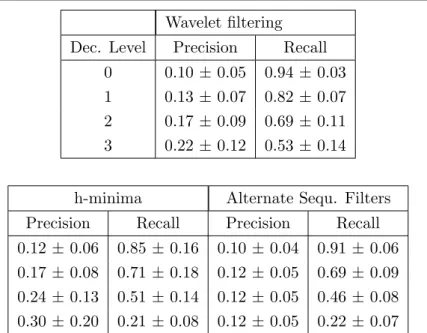
3.1 Results of the wavelet based algorithm on the BSD for each decomposition
level . . . 45
4.1 A summary of color features. . . 51
4.2 A summary of geometric features . . . 52
4.3 A summary of contour features . . . 54
4.4 A summary of texture features . . . 54
5.1 Results of the Eikonal and the normalized cut algorithm on the test images of the BSDS500 . . . 98
5.2 Results of the Eikonal, the normalized cut and SWA algorithm on the test images of the BSDS500 . . . 101
5.3 Results of the Eikonal, the normalized cut and SWA algorithm on the test images of the BSDS500 . . . 102
6.1 Results of cloud sky segmentation with 800 superpixels. . . 113
6.2 Results of cloud sky segmentation with 200 superpixels. . . 113
Introduction
Background
Image segmentation, sometimes referred to as perceptual grouping, constitutes an im-portant area of research in image processing. It refers to the process of partitioning an image into several regions that are perceptually similar, because they share common colors or textures, or because they correspond to objects of interest in the image. This research topic has been widely studied over the years and remains currently very active.
Segmentation results are useful in many computer vision applications. In stereo and motion estimation problems, segments often provide regions of support for computing cor-respondence. In higher level problems such as recognition or image indexing, segmentation techniques are classically used to solve figure-ground separation or recognition by parts problem.
It is important to note that image segmentation is a distinct task from image clas-sification. For the latter, the seeked objective is to assign to each pixel the label of the class to which it belongs. The vision of image segmentation is more global and seeks to identify regions formed by pixels that share similar characteristics and to divide the whole image into regions corresponding to different parts in the scene. The distinction becomes blurry when considering end-to-end semantic segmentation tasks, where the segmentation is achieved through the classification of pixels.
Segmentation is also different from contour detection, which aims at finding the con-tours in the image. Concon-tours indicate the existence of different objects, but not all the contours are useful depending on the scale of interest or on the vision task under consid-eration. Contour detection is often used as a first step for segmentation. Nevertheless, an actual segmentation is only obtained when relevant contours have been selected and when some algorithm has grouped them into closed contours.
Image segmentation is a challenging task and there is currently no comprehensive
Figure 1.1 – Image 118035 in BSDS500 database [Mar01] and its five ground truth images segmented by different human subjects.
theory in this field, not least because a given segmentation is often aimed at a specific application. The methods based on gradient can be disturbed by noise or textured patterns in the image, thus producing a contour where is actually not. In addition, it is difficult to find a contour if two regions share similar colors or gray levels, or when a contour corresponds to small gradient. Moreover, the result of a segmentation depends on the applications and on the scale of the objects of interest. Even human based segmentations are characterized by a significant variability in terms of result. A hierarchical segmentation, which provides a set of segmentations adapted to distinct scales, is therefore desirable for some image processing tasks.
Literature review
A large amount of research has been conducted on image segmentation, based upon a variety of techniques including active contours, clustering, region splitting or merging, etc. These methods can be roughly classified into contour based methods and region based methods, or local methods and global methods. For contour based methods, contour detection algorithms are first used to obtain candidate contours. Then one has to find a way to close the contours as in [RFM05;Arb09]. For region based methods, the image is oversegmented into small regions, which are merged hierarchically to get a segmentation.
In this section, we briefly review the vast literature on image segmentation. We distin-guish, somewhat arbitrarily, between active contours, morphological algorithms, clustering algorithms, graph-based algorithms, and machine learning based algorithms. New trends in image segmentation, including CNN based segmentation and semantic segmentation are also briefly discussed. Rather than describing in depth each approach to image segmenta-tion, this section was written to illustrate the huge variety of mathematical tools that are classically used to perform image segmentation.
Active contours approaches
Active contour algorithms work by simulating the evolution of a closed curve on the image. These algorithms need user provided curve for initialization, and rely on energy minimization or on forces related to the local properties in the image to recover the contours of interest.
In 1988, Kass et al. [KWT88] proposed an algorithm based on the minimization of the energy of splines for contour detection, referred to as snakes. The energy functional comprises three terms: one term corresponding to some internal energy, one term leading to image forces and one term leading to external constraint forces, respectively. The internal energy term imposes a piecewise smoothing on the curve. Image forces push the curve towards relevant image features, such as lines, edges and subjective contours. An initial curve is placed near the desired contour, adding an external constraint to the snake. Nearby edges are then localized by the algorithm through the minimization of the energy term.
Malladi et al. presented in 1995 [MSV95] a level set approach for shape modeling. In their approach, an initial contour is provided by the user, which lies inside a shape, or encloses all the constituent shapes. Then the front propagates as the zero level set of a higher dimensional function, inward or outward in its normal direction, with a speed related to the local image gradient to find the contours of interest. Compared to snakes,
this approach is able to recover shape with protusions, and the front can be easily splitted to recover more than one object.
Morphological segmentation
Morphological segmentation approaches provide well localized and closed contours, usually at the price of significant oversegmentation. A large amount of research has been conducted over the years to reduce the oversegmentation.
The archetypal morphological technique for image segmentation is the watershed al-gorithm, which was introduced in 1979 by Beucher and Lantu´ejoul [BL79] for contours detection in gray level images. It is non-parametric and provides closed contours. The algorithm is inspired by the geographic notions of catchment basins and watersheds, and provides mathematical definitions of these notions based on the geodesic distance. The contours are defined as the watersheds of the variation function (gradient modulus) of the gray levels. Applications including fractures detection in steel and bubble detection in radiography are detailed in the original article.
In 1990, Meyer and Beucher [MB90] wrote a review on image segmentation methods based on the watershed transform and the homotopy modification. The oversegmentation problem is solved by introducing markers within the objects of interest. Lower-complete and upper complete-functions are defined to solve the undersegmentation problem due to broken contours and overlapping particles, that take into account shape information. Methods for markers design under various situations are illustrated by examples of elec-trophoresis gel, traffic lane segmentations and images in other domains. The watershed algorithm is also extensively used in medical imaging applications [Pas07].
Later, Beucher [Beu94] proposed a hierarchical segmentation algorithm based on the mosaic image and the waterfall algorithm to reduce the oversegmentation produced by watershed algorithm. A valued graph is constructed from the mosaic image. Each edge in the valued graph is weighted by the minimal value of the gradient on the corresponding image boundary. A hierarchical image is obtained by assigning to each catchment basin the minimum gradient of its surrounding arcs. The segmentation is computed by applying a watershed transform on the hierarchical image. The waterfall algorithm selects signif-icant minima through reconstruction of the gray level function by the watershed. These significant minima are used as markers for the watershed. The conclusion is that the wa-terfall algorithm is more general than the hierarchical algorithm, and easier to use than the dynamics.
In 2007, Angulo and Jeulin [AJ07] introduced a stochastic segmentation method based on the watershed algorithm. In their method, M realizations of N random germs are
generated independently according to Poisson distribution, resulting in M marker images. Next, a watershed segmentation is computed with the M marker images and a probability density function of contours is calculated using a Parzen window method. The probability density function is then segmented using a volumic watershed transform to obtain the
R most significant regions. The random generation of markers helps to select contours
that are robust to the variations of the segmentation conditions. Two other random germs frameworks are discussed in [AJ07], namely regionalised random germs, and uniform random germs leveling. The last framework yields the best results and outperforms the standard watershed algorithm when the aim is to segment complex images into a few regions. One of the main difficulties associated with the stochastic watershed algorithm is the computation of the probability density function for the contours. In 2014, [MH14] presented a quasi-linear algorithm enabling to compute exactly the probability density function.
Two improvements of the stochastic watershed were proposed in 2013 by Berander et al. [Ber13]: adding uniform noise to the input image at every iteration, and distributing the markers using a randomly placed uniform grid (with random offset and rotation). With these modifications, images with larger variabilities in region size are better segmented, the result is less sensitive to the number of markers, and the depth threshold becomes easier to set. The F-measure obtained on a database of fluorescent microscope images of nuclei was largely improved with this method.
In 2015, Meyer [Mey15] presented a hierarchical segmentation strategy based on stochas-tic watershed, and provided various strategies to construct hierarchies. In his study, a minimum spanning forest is used to construct a hierarchy based on prioritized markers. The strength of a contour is estimated by the level of hierarchy for which its two associated regions merge. Various features including size, contrast, orientation, color, and texture features can be considered with different hierarchies. One has nevertheless to tailor the hierarchy according to the problem at hand.
During the same year, Franchi and Angulo [FA15] proposed a fully unsupervised multi-scale approach to address the drawback of stochastic watershed of enhancing insignificant contours in complex images, referred to as bagging stochastic watershed (BSW). The gPb gradient in [Arb11] is employed when calculating the probability density functions. Probability density functions at different scales are combined to compute the BSW. This algorithm is evaluated on the BSDS dataset and compared with other stochastic watershed algorithms. The ISW approach [Ber13] achieves the best F-measure of all stochastic watershed based approaches.
Clustering algorithms
Another family of segmentation methods is based upon the notion of clustering or grouping. It is intuitive to regard segmentation as a clustering problem, since pixels with similar color and texture are more likely to belong to the same object. Mean-shift and other mode finding techniques, such as K-means and mixtures of Gaussians try to find clusters in the distribution of points in the feature space to compute the segmentation [Sze11].
In 2002, Comaniciu and Meer [CM02] proposed a general nonparametric technique for multimodal feature space analysis, which is able to delineate arbitrarily shaped clusters based on mean shift. Mean shift is defined as the difference between the weighted mean of points and the center of the density kernel. Comaniciu and Meer proved that recursive mean shift can be used to detect the modes of the density. The application of mean shift based mode detection in image segmentation with joint spatial-range domain representa-tion overcomes the issue of gray or color clustering algorithms of oversegmenting small gradient regions. The only parameter to set is the resolution of analysis, which depends on the vision task.
Paris and Durand described in 2007 [PD07] a new fast algorithm for mean-shift im-age segmentation computation based on Morse theory, and introduced a way to build a segmentation hierarchy. Gaussian kernels are employed for density estimation, and the density function is computed on a regular grid. The mode extraction is done explicitly by assigning to each pixel the label of the corresponding maxima, in decreasing order of density. A persistence of boundary based on the topological persistence is defined, and clusters with boundary persistence less than a threshold are merged for simplification. A segmentation hierarchy is therefore obtained by gradually increasing the threshold. The boundary persistence can be modified to account for color information, depending on the application. PCA can be used to reduce the dimension of the feature space therefore accelerating the computation.
Clustering algorithms can also be employed for superpixels generation, as Simple Linear Iterative Clustering (SLIC) superpixels [Ach12] proposed by Achanta et al. based on K-means clustering algorithm. SLIC is one of the state-of-the-art superpixel algorithms. More details on this algorithm can be found in section2.2.
Graph-based approaches
Graph based segmentation methods transform image segmentation problems into graph partitioning problems by representing an image by a graph constructed by linking adjacent
pixels or regions. The aim is to segment an image into regions with low variability within each region and high variability between regions.
In 2000, Shi and Malik [SM00] proposed a novel graph-theoretic criterion to measure the effectiveness of an image partition, the normalized cut, and an efficient technique for the minimization of this criterion based on a generalized eigenvalue problem. This algorithm extracts global impression and obtains good results on static images and motion sequences.
In 2004, Felzenszwalb and Huttenlocher [FH04] introduced a graph-based image seg-mentation method based on pairwise region comparison. In their approach, pixels are merged according to their intensity differences across boundaries and between neighboring pixels within each region. The segmentation criteria are adaptively adjusted to take into account the variability in neighboring regions. Two different kinds of local neighborhoods, namely grid graphs and nearest neighbour graphs, are tested for graph construction. The advantage of this approach is that it preserves details in low-variability regions while ig-noring details in high-variability regions.
The literature on graph based approaches, including minimum spanning tree based algorithms and graph cut algorithms, is reviewed in greater details in section5.1.
Machine learning based methods
Learning based methods have increasingly gained popularity for performing image segmentation over the past 20 years. In these methods, machine learning algorithms, such as linear regression, support vector machines (SVM) or random forests are used to combine various cues, providing a merge probability for region merging, or a measure of similarity for graph based approaches for image segmentation. Machine learning based methods can be generalized to other kinds of images by changing the training images. The choice of features is essential for machine learning based algorithms.
In 2003, Ren and Malik [RM03] proposed a two class classification method for group-ing. In this work, natural images segmented by humans are taken as positive examples. Varieties of image features from the classical Gestalt cues, including contour, texture, brightness and good continuation features are calculated for both inter-region and intra-region cases. The effectiveness of each feature is evaluated through information entropy, and the conclusion is that boundary contour is the most informative grouping cue. A logistic regression classifier is used for learning the algorithm parameters. A globally op-timized segmentation is found by using a random search based on simulated annealing. The method is tested on the Corel Image base [WLW01].
In 2004, Martin et al. [MFM04] proposed a natural image boundaries detection method
where local brightness, color, and texture features, including oriented energy, brightness gradient, color gradient, and texture gradient are employed. A methodology for bench-marking boundary detection algorithms is also defined in their study. Human-marked boundaries from the Berkeley Segmentation Dataset [Mar01] are used as ground truth. A logistic regression classifier is trained to predict the posterior probability of a pixel being on a boundary based on the combination of cues. Their results reveal the importance of texture treatment in natural images boundaries detection.
In 2006, Doll´ar et al. [DTB06] presented a novel supervised learning algorithm for edges and boundaries detection. In the proposed algorithm, an extension of probabilistic boosting trees is trained based on tens of thousands of simple features at multiple scales and orientations from large image patches centered at different locations, taking into account low, mid, and high level information. The probability for each location to belong to a boundary is calculated independently. The performance of this method on the BSDS300 dataset is comparable to that of Pb [MFM04]. Good results are also achieved in object boundary detection and rode detection applications.
A machinery for contour detection and hierarchical segmentation was proposed in 2011 by Arbel´aez et al. [Arb11], where multiple local cues (brightness, color and texture gradi-ents) at multiple scales and orientations are combined into a globalization framework to predict a probability of boundary. An Oriented Watershed Transform (OWT) and Ultra-metric Contour Map (UCM) are then employed to close the contours and to produce a hierarchical segmentation. This algorithm significantly outperforms competing algorithms on each dataset (BSDS, MSRC, PASCAL 2008) and for each considered benchmark crite-rion.
In 2012, Alpert et al. [Alp12] presented an image segmentation approach by proba-bilistic bottom-up aggregation. The proposed algorithm starts from a graph where each pixel in the image is represented as a node. Pixels are then gradually aggregated to pro-duce larger regions, according to a probabilistic model that considers the distribution of intensity difference and of texture difference to output a probability of merging adjacent regions. A graph coarsening scheme is integrated for merging. A novel evaluation scheme is proposed and this algorithm achieves a high average F-measure with the least number of fragments both in one-object and two-objects data set.
In the same year, Arbel´aez et al. [Arb12] proposed a new design for region-based object detectors, which can integrate top-down information from a scanning-windows part model, and global appearance features (shape, color and texture). This design focuses especially on the recognition of challenging articulated categories. This algorithm achieves competitive performance on PASCAL segmentation challenge and the highest accuracy on articulated objects VOC2010 dataset.
In 2014, Arbel´aez et al. [Arb14] proposed a unified bottom-up hierarchical image seg-mentation and object candidate generation algorithm named Multiscale Combinatorial Grouping (MCG). In their approach, they firstly construct a multiresolution image pyra-mid by subsampling and supersampling the original image. A hierarchical segmentation is then computed at each scale of the pyramid, and the hierarchies are finally aligned and combined into a single segmentation hierarchy. A classifier is trained to combine the contour strength from different scales. Compared to [Arb11], more cues including sparse coding on patches and structured forest contours are added for single scale segmentation, and an efficient normalized cut algorithm is designed to accelerate the globalization step. This approach provides state-of-the-art segmentations and object candidates on BSDS500 and PASCAL 2012 datasets.
In 2015, Doll´ar and Zitnick [DZ15] proposed a generalized structured learning approach for edge detection, taking advantage of inherent structures in image patches by using structured forests. This approach is different from the aforementioned methods, in the sense that it detects edges by predicting a segmentation mask for each image patch. A feature vector comprising color, gradient magnitude at various scales and orientations and differences of downsampled pixel pairs is extracted for each patch. A mapping function is designed to map the structured labels of a patch to an intermediate space where similarity can be approximated by the Euclidean distance. A structured forest classifier is trained for edge map prediction. The edge maps can be sharpened using local color cues. This approach achieves state-of-the-art edge detection results on the BSDS500 dataset and NYU depth dataset, and has realtime performance.
CNN based image segmentation
For machine learning based image segmentation, it is essential to involve global in-formation, or information from multiple scales. The performance of the segmentation depends indeed strongly on the set of selected features. To improve the performance of segmentation, complicated handcrafted features are involved in state-of-the-art algorithms [Arb11; Arb14]. The application of convolutional neural networks on segmentation can potentially relieve us from designing and selecting features. By convolving an image with learned filters, nonlinear mapping and pooling, a feature map can be produced comprising both low, mid and high level features.
Their performance and ease of use make CNN based segmentation algorithms popular nowadays. In this chapter, we do not intend to give a thorough description of the literature on deep learning based segmentation methods, and we briefly mention a few classical articles in this section. A thorough review can be found in [Gho19].
One of the first articles on CNN based segmentation was published in 2013 by Farabet
et al. [Far13], who presented a scene parsing approach based on a multiscale convolutional network. In their work, a three-staged ConvNet is applied to each scale of a Laplacian image pyramid for extracting features vectors. Network weights are shared across scales to enforce the scale-invariance of the learned features. Then, features maps from multiple networks are upsampled and concatenated into a map of features vectors, characterizing regions of multiple sizes centered on each pixel. The second step of the algorithm consists of a postprocessing step to ensure the spatial consistency of the scene labeling. Three strategies are tried: averaging class distribution within superpixels, minimizing the energy of a Conditional Random Field constructed from the labeling and applying a multilevel cut with a class purity criterion. This approach yielded record accuracies on the SIFT Flow dataset and on the Barcelona dataset.
R-CNN (regions with CNN features) [Gir14] was proposed in 2014 for object detection and semantic segmentation based on region proposals. Part of the architecture of R-CNN involves an AlexNet architecture pre-trained on the ILSVRC dataset for object detection. Region proposals are generated by selective search, and wrapped to the input size of the CNN. A fixed-length feature vector is then extracted for each region. A linear SVM is finally trained for each class for classification. The extension of R-CNN to segmentation also achieves state-of-the-art performance on VOC 2011. This article adapts the CNN for image classification to object detection task, and shows the effectiveness of supervised pre-training and domain specific fine-tuning, offering a practical solution for tasks with small amount of labeled data for instance object detection.
In [LSD15], fully convolutional networks were proposed for semantic segmentation, which adapt the learned representations of classification networks to achieve an end-to-end segmentation, accepting arbitrary-sized inputs. In this approach, the fully connected layers of classification networks are notably converted into convolution layers. The feature map is upsampled to the size of inputs by deconvolution. To improve the resolution of the prediction, a skip architecture is designed to combine the semantic information from a deep layer with appearance information from a shallow layer. This algorithm improves the state of the art on PASCAL VOC 2011, NYUDv2 and SIFT Flow dataset, and is quick for inference compared to patch based segmentation.
Objective of the thesis
As pointed out in the previous section, state-of-the-art segmentation algorithms make extensive use of machine learning techniques. CNN-based algorithms require to be trained on a large number of segmentation examples, for instance on image datasets including Common Objects in COntext (COCO) [Lin14] or PASCAL VOC [Eve10], which comprise tens of thousands of annotated images. Algorithms based on more traditional machine
learning methods where features are mostly handcrafted, like the gPb algorithm, can be trained on smaller datasets. gPb is for instance trained on the Berkeley Segmentation Dataset, which contains 200 images for training.
In a number of practical applications, notably including images obtained in remote sensing or materials science applications, the lack of annotated images constitutes a signif-icant issue if one wants to apply machine learning based image segmentation algorithms. A common solution for applying deep learning algorithms when few training data is avail-able is to fine-tune an architecture of neural network pre-trained on a large database of images, a technique referred to as transfer learning in the literature. The idea behind transfer learning is that the pre-trained neural network will have identified useful features on the large dataset of images on which it is pre-trained, and that these features remain relevant for processing the new set of images. Nevertheless, due to the specificity of the images gathered in materials engineering applications or on remote sensing observations, transfer learning techniques largely remain inoperative.
In this PhD thesis, our objective is to work on the development of algorithms that can be trained to perform the segmentation of a dataset constituted of similar images with only a few annotated images as training examples. Such datasets are commonly obtained when experiments are conducted in materials science.
Our proposed methodology is based on a region segmentation approach. More pre-cisely, starting from a superpixel partition of the image, we propose a merging algorithm which gradually merges the initial regions until an actual segmentation is obtained. The work presented in this PhD manuscript focuses on the two key aspects of the proposed methodology, namely the superpixel generation and the superpixel merging.
Thesis outline
In the first part of the manuscript, corresponding to chapters 2 and 3, we introduce two novel algorithms that can be used to compute a superpixel partition and a hierar-chical superpixel partition of the image, respectively. The superpixel algorithm presented in chapter 2 makes use of the Eikonal equation to generate the superpixel partition, in a way relatively similar to the algorithm introduced by Buyssens et al. [Buy14b]. The algo-rithm compares favorably to other state-of-the-art superpixel algoalgo-rithms on the Berkerley Segmentation Dataset. In chapter 3, which is somehow independent from the rest of the manuscript, we describe a segmentation algorithm based on the wavelet transform and on the watershed transform that yields a hierarchical superpixel segmentation of the image. The developed algorithms have been published at ISMM 2017 [FCF17] and ISMM 2019 [CF19] conferences.
In the second part of the manuscript, corresponding to chapters 4 and 5, we present an algorithm performing superpixels merging based upon learned similarities between ad-jacent regions. The superpixels merging approach is conducted in the framework of graph theory. More precisely, a region adjacency graph is computed from the superpixel parti-tion. Each superpixel in the partition corresponds to a node in the graph, while each pair of adjacent superpixels are linked by an edge. The edges are weighted by a dissimilarity measure, which is taken to be the probability that both superpixels belong to distinct seg-ments of the final segmentation. A machine learning algorithm is used for estimating the dissimilarity, which takes as input features various characteristics of the regions including their respective colors and textures, or the strength of the gradient at the boundary. The learning process, as well as the characteristics used to compute the similarity, are discussed in chapter 4.
In chapter 5, we propose a method using the Eikonal equation to perform the clustering of the region adjacency graph, in a similar way to the superpixel approach proposed in chapter 2. The Eikonal equation is notably adapted to the specific setting of graphs. The proposed approach is finally compared to classical approaches for performing region mergings including the normalized cut algorithm [SM00] and the segmentation by weighted aggregation [Alp12]. The comparison is conducted on the Berkeley Segmentation Dataset.
To conclude the manuscript, we present in chapter 6 the application of our methodology to a dataset of cloud images, where our approach yields state-of-the-art results with a limited number of training instances. Conclusions are finally drawn in the last chapter.
Fast marching based superpixels
Superpixel algorithms refer to a class of techniques designed to partition an image into small regions that group perceptually similar pixels. Superpixel segmentations are often used as a preprocessing step for computer vision tasks, such as image segmentation [FVS09], object detection [Yan15], tracking [Wan11; YLY14], depth estimation [ZK07] or object classification, to simplify the computation for further processing or to provide computational support for features.This chapter introduces an algorithm based on the fast marching method to compute the superpixel partition of an image. The fast marching algorithm finds several applica-tions in mathematical morphology and stochastic geometry [DD03;Fig16;Bor18; Fig19]. In section 2.1, we discuss general properties of superpixels and we provide a review of the main state-of-the-art superpixel algorithms; in section 2.2, we elaborate on the fast marching algorithm and we describe in greater detail the proposed fast marching based superpixel (FMS) algorithm. The results of the FMS are presented in section 2.3 and compared with other superpixel algorithms. We draw conclusion and present perspectives in the last section.
Introduction
The idea of over-segmenting an image into regions for further processing existed long before the term “superpixel” was coined, for example in [MM97]. It was in [RM03] that this term was first introduced in the context of image segmentation.
Superpixel segmentations are over-segmentations which obey certain properties, in-cluding:
1. Boundary adherence: superpixels should preserve the boundaries in the image [Ach12;SHL17]. This property is for instance of paramount importance for segmen-tation applications. Several metrics have been defined in the literature to quantify boundary adherence, including boundary recall, which characterizes the amount of
boundary pixels that are recovered by the segmentation algorithm within a tolerance of 1 or 2 pixels, and undersegmentation error, which quantifies the “leakage” of the superpixels crossing an actual boundary of the image.
2. Regularity, smoothness: The shape of the superpixels should be regular and their boundaries should be smooth where there is not an object boundary. Obviously, algorithms returning superpixels with highly tortuous contours are more likely to exhibit high adherence to boundaries, but the resulting partition can hardly be considered to be satisfactory. Criteria including average compactness or superpixels contours density are classically used to characterize the shape of the superpixels [MDW14;Mac15;SHL17].
3. Efficiency: Superpixels should be fast to compute and memory efficient. Since superpixel segmentation is often used as a preprocessing step to simply further pro-cessing, its application should not consume much time, especially for real time tasks.
Literature review
A lot of research has been conducted on superpixel algorithms. In [SHL17], a thorough literature review of this field is provided, as well as a benchmark for comparison. [Wan17] provides a simple classification of these algorithms between graph-based methods and clustering based methods.
Graph based superpixels
Graph based methods build upon a graph representation of the image. In this repre-sentation, each pixel constitutes a node of the graph and all couples of adjacent pixels are linked by an edge. The weight of an edge is usually interpreted as the similarity or dissim-ilarity between neighboring pixels, defined by their intensity, color or spatial differences. In this way, the segmentation problem is transformed into a graph partitioning problem. Classical graph-based algorithms for superpixels generation include the normalized cut al-gorithm (NC) [SM00; Mal01] and the efficient graph-based segmentation algorithm (GS) [FH04].
To give a general view of graph based superpixel algorithms, we elaborate on the GS algorithm. In this approach, a graph is constructed either by connecting pixels in a 8-connected neighborhood, or by connecting nearest neighbor pixels in a feature space. In the first case, the weight of an edge is taken to be the absolute value of the intensity difference; in the second case, the weight can be chosen to be the Euclidean distance or other form of distance defined on the features space. Then, the edges of the graph are sorted in a non decreasing order according to their weights and visited in this order. At
each iteration, if two nodes vi and vj are not in the same component, and if the weight wij
is smaller than the minimum internal difference plus a threshold of each component Ci, Cj, meaning that the inter-region difference is smaller than the within-region difference,
the two components are merged. The internal difference of a component is defined as the maximum weight of its minimum spanning tree. The threshold term can be designed according to the size or shape of preferred regions. This procedure is iterated until all edges are processed. The complexity of the algorithm is O(m log m), where m is the number of edges.
Some graph based algorithms produce superpixels through the optimization of an ob-jective function. Entropy rate superpixels (ERS) [Liu11] is one of these algorithms that achieves state-of-the-art performance. An objective function based on entropy rate is de-fined, where entropy rate is the asymptotic conditional entropy of a random process, which measures the remaining uncertainty after observing its past trajectory. A balancing term is introduced in the objective function to favor superpixels with similar sizes. The overseg-mentation is obtained by selecting edges that form a partition with K connected subgraphs. It is proved that the optimization of this objective function can be done efficiently by a lazy greedy algorithm with a complexity of approximately O(|V | log |V |), where V is the set of the graph vertices (pixels). This algorithm achieves better performance both in undersegmentation error and in recall than GS on the Berkeley segmentation benchmark [Mar01].
Clustering based superpixel algorithms
Clustering based methods for superpixel segmentation proceed by iteratively refin-ing clusters of pixels until some convergence criterion is met. Clusterrefin-ing based methods notably include mean shift [CM02], watershed [VS91; BL79], turbopixel [Lev09], simple linear iterative clustering (SLIC) [Ach12; AS17] and waterpixel [MDW14; Mac15; CJ19] algorithms, respectively.
The simple linear iterative clustering (SLIC) algorithm [Ach12;AS17] is an archetypal example of clustering based algorithm. Due to its ease of use and its good performance, SLIC is ranked among the most used algorithms for computing a superpixel segmentation. In addition, the SLIC algorithm has a linear complexity, its implementation is available [Ach12] and it offers the possibility to weight the trade-off between boundary adherence and shape or size similarity.
SLIC constructs a superpixel partition by applying a k-means clustering algorithm on local patches of the image. During initialization, K cluster centers locations are selected on the image using a grid with uniform spacing S. Each pixel is then associated to the closest cluster center in the image according to a distance involving the color proximity
and the physical distance between the pixel and the seed, respectively. The search for similar pixels is restricted to a neighborhood of size 2S by 2S around each cluster center. After the assignment step, the K cluster centers are updated. The color and the location associated to the cluster centers are set equal to the average color and location of the pixels of the cluster. The L2 distance between the previous and the new locations is used to compute a residual error E. The aforementioned procedure is iterated until the error E converges. The clusters of pixels obtained after this procedure are usually not connected. A post-processing step is therefore applied to reassign the disjoint pixels to nearby superpixels.
Eikonal based region growing Clustering (ERGC) [Buy14b;BGR14;Buy14a] is a clus-tering based superpixel algorithm that produces superpixels by solving the Eikonal equa-tion which describes the label propagaequa-tion from initial seeds, with a velocity based on color distance between the pixel and the seed. It achieves state-of-the-art performance and is efficient to calculate, with a complexity of O(n log n), n being the number of pixels in the image. Another advantage of ERGC compared to SLIC is that no post-processing is required to obtain connected superpixels.
Other trends
Other superpixel algorithms are based on energy maximization. Superpixels Entracted via Energy-Driven Sampling (SEEDS) [Ber12] is one such algorithm that can be calculated in real time. Van den Bergh et al. proposed an objective function composed of two terms, one based on the color density distribution of each superpixel, the other, optional, used as a smoothing term based on the histogram of superpixel labels in a patch. This objective function is optimized by hill-climbing optimization, namely to make small local changes of superpixel labels at each iteration. The optimization is done in a hierarchical manner, by moving large blocks of pixels in early iterations, latter small block of pixels, at last single pixels to neighboring superpixels. It can achieve better boundary adherence than SLIC and ERS, and is faster to calculate. The main disadvantage of SEEDS is that it yields highly irregular boundaries.
Most superpixel algorithms make use of color and spatial information. Recently, several studies have demonstrated that using texture information could improve the superpixel performance. Xiaolin Xiao et al. [XGZ17] proposed to introduce both texture and gradient distance terms in SLIC’s distance formula. In their work, the weight of each term is adapted to the discriminability of the features in the image. Their algorithm achieves better performances than state-of-the-art algorithms including SLIC and LSC [LC15]. Giraud et al. [Gir19] proposed to measure the texture distance between a pixel and a superpixel seed by considering the average distance between a square patch around that pixel and similar patches inside the superpixel found by a nearest neighbor method.
The ERGC algorithm gives promising results, but there are still some aspects worth of researching. Firstly, we can note that the position of the initial seeds do not change during the process, while more seeds might be needed for complicated regions. Secondly, it might be interesting to take the texture information into consideration to compute the image partition.
In the next subsection, we introduce a novel clustering-based algorithm for generating a superpixel partition of a given image termed fast-marching based superpixels (FMS). Following an idea originally introduced for the Eikonal-based region growing for efficient clustering algorithm (ERGC) [Buy14b;Buy14a;BGR14], we rely upon the Eikonal equa-tion and the fast marching algorithm to assign the pixels of the images to the relevant clusters.
Eikonal equation and fast marching algorithm
A clustering based superpixel algorithm generally comprises 2 steps:
1. Initialization. A group of initial seeds should be provided as a basis for clustering. 2. Clustering. The pixels are clustered to their corresponding seeds based on the
dis-tance. The seeds can be updated after a pass of assignment. Thus the superpixel segmentation transforms to the following problem: knowing the position and proper-ties of initial seeds, how can we assign a label to each pixel, in order for the resulting partition to have “good” properties (e.g. boundary recall, compactness, etc.). The idea behind the Fast Marching Superpixel (FMS) algorithm is to draw an analogy between waves propagating in a heterogeneous medium and regions growing on an image at a rate depending on the local color and texture. Instead of using clustering algorithms, such as k-means clustering or DBSCAN clustering [She16], we propagate the labels of the seeds with a process that can be described by the Eikonal equation. Fast computational algorithms are available to approximate the solution of the Eikonal equation, including the fast marching algorithm [Set96; Set99a; DD03]. We elaborate on the Eikonal equation and the fast marching algorithm in this section.
Eikonal equation
The Eikonal equation is a non-linear partial differential equation which describes the propagation of waves in a medium. It finds notable applications in fields including geo-metrical optics or geophysics. In this section, we will first present classical results relative to the Eikonal equation on continuous domains, before studying its generalization to dis-cretized domain.
Figure 2.1 – Propagation front and level sets.
Eikonal equation on a continuous domain
Let Ω denote some open domain in R2. In what follows, we consider a front Γt
propa-gating on Ω in the normal direction at a velocity u := u(x) at every point x ∈ Ω. Obviously, the equation describing the propagation of the front is
dΓt
dt (x, t) = u(x)nΓ(x), (2.1)
where nΓ is a unitary vector directed toward the direction normal to the propagation front.
A popular approach to solve equation (2.1) is to rely on level sets.
Definition 2.3.1. A level set L on Ω ⊂ R2 is a subset of Ω where some real valued function v : Ω → R takes a constant value c ∈ R
L := {x | v(x) = c}. (2.2)
For t ≥ 0, the propagation front Γt can be represented as the level set of a function v : Ω × R → R such that
∀t ≥ 0, Γt:= {x|v(x, t) = 0}. (2.3)
Proposition 2.3.1. Let us consider a close propagation front Γt and a function v such
that v(x, t)
< 0 if x is inside the area delimited by Γt
= 0 if x ∈ Γt
> 0 if x is outside the area delimited by Γt
(2.4)
Then, the outward normal direction with respect to the propagation front is given by
nΓt :=
∇v(x, t)
k∇v(x, t)k, (2.5)
At this point, let us consider a trajectory t → y(t) ∈ Γt. Necessarily, for t ≥ 0, we have
v(y(t), t) = 0. (2.6)
Hence, by differentiating with respect to t, we can easily show that the function v is the solution of the partial differential equation
∂v
∂t(y(t), t) + ∇v(y(t), t) · ˙y(t) = 0. (2.7)
According to proposition2.3.1, we have
˙
y(t) = u(y(t))nΓt= u(y(t))
∇v(x, t)
k∇v(x, t)k. (2.8)
This leads to the so-called Eikonal equation defined for all x ∈ Ω by
∂v
∂t(x, t) + u(x)k∇v(x, t)k = 0. (2.9)
In this work, we will present a method for solving the Eikonal equation through a stationary approach. To that end, let us denote by x → T (x) the function associating to each point x ∈ Ω the arrival time of the propagation front Γt. In mathematical terms, T
is defined by the implicit equation
T (y(t)) = t, (2.10)
for all trajectory t → y(t) ∈ Γt. When we differentiate this equation with respect to t, we
obtain the equation
u(y(t))||∇T (y(t))|| = 1. (2.11) This equation can be solved for the entire domain Ω, becoming
||∇T (x)|| = 1
u(x), ∀x ∈ Ω. (2.12)
Boundary conditions are usually specified on the boundary ∂Ω of the domain. One usually considers a function g defined on the boundary ∂Ω so that t(x) = g(x) for all x ∈ ∂Ω. Usually, the function g is taken to be identically 0. Hence, the stationnary Eikonal equation
becomes ||∇t(x)|| = 1 u(x), ∀x ∈ Ω t(x) = 0, ∀x ∈ ∂Ω. (2.13)
For all x in Ω, the solution t(x) of equation (2.13) can be interpreted as the minimal time required to travel from x to the domain boundary ∂Ω. For all x in Ω, we denote by
d the geodesic distance function defined by d(x, ∂Ω) = inf
y∈∂Ω||x − y||, (2.14)
where ||x − y|| is the geodesic distance between x and y. Proposition 2.3.2below relates the distance function d to the solution of the Eikonal equation on the domain Ω.
Proposition 2.3.2. [Set96] Let Ω be a subset of the Euclidean space R2. Then, the distance function d(·, ∂Ω) is differentiable almost everywhere, and its gradient satisfies the Eikonal equation
||∇d(x, ∂Ω)|| = 1 with initial conditions d(x) = 0, ∀x ∈ ∂Ω.
In other words, the Eikonal equation allows us to compute the shortest distance be-tween any point x of the domain Ω and the boundary ∂Ω.
Eikonal equation on a discretized domain
Let us consider the discretization of the Eikonal equation on a domain Ω ⊂ R2. We assume that Ω can be discretized on a regular grid.
Figure 2.2 – An illustration of 4 connected neighborhood.
We rely on the finite difference approximation formula as in [Set96] to approximate the gradient term at grid point (i, j):
||∇t(i, j)|| ≈qmax(D−xij , −Dij+x, 0)2+ max(D−y
ij , −D +y ij , 0)2 = 1 uij , (2.15)
where uij is the velocity of the wave at (i, j). D−xij , D+xij , D
−y
ij , and D
+y
ij are partial
derivatives, and we use the standard finite difference notation in 2D:
D−xij = tij − ti−1,j ∆t , D +x ij = ti+1,j− tij ∆t (2.16)
For simplicity’s sake, we assume that ∆t = 1. Thus ||∇t(i, j)||2 = max(t
i,j− ti−1,j, ti,j− ti+1,j, 0)2
+ max(ti,j− ti,j−1, ti,j− ti,j+1, 0)2
(2.17)
Using the gradient discretization (2.17), the Eikonal equation becomes max(ti,j− ti−1,j, ti,j− ti+1,j, 0)2+
max(ti,j− ti,j−1, ti,j− ti,j+1, 0)2 =
1
u2
i,j
In this equation, the only unknown is the arrival time ti,j at point p := (i, j). We have
max(ti,j− ti,j−1, ti,j − ti,j+1, 0)2=
max(ti,j − min(ti,j−1ti,j+1), 0)2.
(2.19)
Hence, ti,j is solution of the quadratic equation
max(ti,j− min(ti−1,j, ti+1,j), 0)2+
max(ti,j− min(ti,j−1, ti,j+1), 0)2=
1
u2i,j.
(2.20)
Eikonal equation on image domain
In this section, we present a clustering algorithm that works by solving the Eikonal equation on the image domain for clustering pixels in order to generate a superpixel par-tition. The image domain is interpreted here as a special case of discretized domain.
In what follows, we adopt the following notations. A pixel in image I is denoted by p and its coordinates by (x, y). We select N seeds or cluster centers locations {s1, s2, ..., sN}
at initialization. The labels of the seeds are then gradually propagated from the labeled pixels to the unlabeled pixels according to the local velocity {u(p)}. On the domain defined by the image, the Eikonal equation therefore reads
||∇t(p)|| = 1 u(p) ∀p ∈ I t(p) = 0 ∀p ∈ ∂I. (2.21)
In this expression, u(p) is the local velocity at pixel p, ∂I corresponds to the subset of the image I constituted by the seeds {s1, s2, ..., sN}, and t(p) is the the minimal time required
to travel from ∂I to pixel p. The velocity u(p) depends on the color and the texture of both the seed and the pixel location p := (x, y).
For all p in I,
t(p) = t(p, ∂I) = inf si∈∂I
t(p, si), (2.22)
where t(p, si) is the minimal traveling time from si to p.
Fast marching algorithm
Fast methods for Eikonal equation include fast marching based methods, fast sweep-ing based methods and other methods. The fast marchsweep-ing method (FMM) is the most commonly used. It was originally introduced to solve the Eikonal equation on a contin-uous domain [MSV95; Set96]. The fast sweeping method (FSM) [FLZ09] is an iterative algorithm that performs Gauss-Seidel iterations with alternating sweeping ordering.
In [G´o19], nine fast methods including FMM, Fibonacci-Heap FMM(FMMFib), Sim-plified FMM (SFMM), Untidy FMM (UFMM), Group Marching Method (GMM), Fast Iterative Method (FIM), Fast Sweeping Method (FSM), Locking Sweeping Method (LSM) and Double Dynamic Queue Method (DDQM) are compared. The comparison is con-ducted under different circumstances, from simple case of empty maps to more complicated problem such as vessel segmentation.
The choice of the method depends on the application. For complex scenarios such as image segmentation, to solve the Eikonal equation with variable speed, their conclusion is that there is not an optimal method. UFMM can work well if properly tuned. SFMM is a safe choice and it is faster than FMM and FMMFib in each case.
In this research, we make use of the traditional FMM for its simplicity of implementa-tion. Other fast methods, especially SFMM, would be worth considering to improve the speed of our algorithm.
Fast marching on a discretized domain
A possible approach to solve the Eikonal equation is to iteratively solve the non-linear equation (2.20) at each location of the grid until some convergence criterion is met. However, this approach involves a significant amount of calculations to be conducted and can be very costly.
An alternative approach is to compute the arrival times outwards from the initial con-ditions by following the front propagation and computing the arrival times in increasing order. This approach leads to the fast marching algorithm and allows to solve equa-tion (2.20) at each location of the grid in a single iteration.
The fast marching algorithm works by partitioning the points of the discretization domain Ω in three subsets during the front propagation:
— The points that have already been reached by the front are grouped into a set referred to as the frozen set.
— The points of the discretization grid that are adjacent to frozen points but have not been reached by the front yet are grouped in a subset referred to as the narrow band, — The remaining points of the discretization grid are grouped in a subset referred to
as the far away set.
Initialization The fast marching algorithm is initialized as follows:
1. An arrival time map is initialized: each point (i, j) in the discretization grid is associated with the arrival time t = +∞, except if it belongs to the domain boundary
∂Ω. In this case, the point (i, j) is associated with the arrival time tij = 0.
2. All points of the discretization grid located at the domain boundary ∂Ω are added to the narrow band. Other points are labeled as far away. Initially, the frozen set is empty.
Iteration At each iteration, the point (i, j) of the narrow band with the smallest arrival time is extracted and labeled as frozen. Arrival times are computed for its neighbors in a 4-neighborhood by solving equation (2.18). Frozen points are used to compute the arrival times in other points, but their arrival time is never recomputed. We can rewrite (2.18) under the general form
max(tij − tA, 0)2+ max(tij − tB, 0)2 =
1
u2ij, (2.23)
where tA = min(ti−1,j, ti+1,j) and tB = min(ti,j−1, ti,j+1). By construction, (i, j) is
adja-cent to at least one frozen pixel. Without loss of generality, we can assume that A belongs to the frozen set and that tA≤ tB. B can be frozen, in the narrow band, or far away (in
the latter case, tB = +∞). Then, we have the following result:
Proposition 2.3.3. Equation (2.23) has a single solution tij satisfying tij > tA.
Proof. The proof is given in the appendixA.1.
Once the arrival time t of a neighbor point (i, j) has been computed, two situations can be encountered:
— When (i, j) is in the narrow band, it has already been associated an arrival time
t0
ij. If the new arrival time tij is smaller than t0ij, then the arrival time is updated.
Otherwise, it remains unchanged.
— When the neighbor point is far away, we add it to the narrow band with the arrival time tij.
Stopping condition The fast marching algorithm stops when the narrow band is empty.
At each iteration of the algorithm, it is necessary to extract the element of the narrow band with the smallest arrival time. The search for the smallest element in the narrow band can significantly enhance the algorithmic complexity of the fast marching approach. To reduce the complexity of the algorithm, a common solution is to store the elements of the narrow band in a binary heap. When using a binary heap structure, the complexity of the fast marching algorithm is in O(N log N ), N being the number of points in the discretization grid. We refer the reader interested in more details on the fast marching algorithm implementation to the original articles [MSV95;Set96;Set99a;Set99b].
Fast Marching Superpixel (FMS)
The idea behind the FMS algorithm is to draw an analogy between waves propagating in a heterogeneous medium and regions growing on an image at a rate depending on the local color and texture. A similar idea was proposed in [Buy14b; Buy14a;BGR14]. However, both approaches differ in several aspects, including the expression for the local velocity as a function of the image content, the use of texture features or the region update during propagation.
Here we adopt the same initialization step as in SLIC, and focus on the clustering step. Instead of using clustering algorithms, such as k-means clustering or DBSCAN clustering [She16], we propagate the labels of the seeds in a process that can be described by the Eikonal equation. In this section, we describe in greater details the implementation of the FMS algorithm.
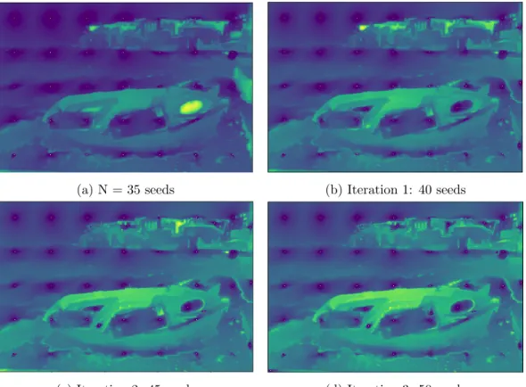
Region growing
Let us denote by K the desired number of superpixels. We initialize the algorithm by selecting N (N < K) seeds on a regular grid. To avoid placing a seed on a boundary, we place the seed at the local minimum of the gradient in a 3 × 3 neighborhood of the nodes on the grid. A similar strategy is used for selecting the initial seeds in the SLIC algorithm [Ach12]. We denote by C(p) the color at pixel p in the CIELAB color space. Similarly, we denote by T(p) a vector of features characterizing the local texture at pixel p.
Initialization The propagation algorithm is initialized as follows: 1. The arrival time map t is initialized:
t(p) = 0 if p ∈ ∂I, +∞ otherwise. (2.24)
2. The label map L is initialized:
L(p) = i if p = si, 0 otherwise. (2.25)
3. The pixels {s1, .., sN} are grouped in a set referred to as the narrow band. All other
pixels are labeled as far away.
(a) Two seeds (b) Compute arrival times of the neighbors of one seed and add them to the narrow band
(c) Choose the pixel with the smallest arrival time (another seed), and freeze its label and arrival time
(d) Calculate and update the arrival times of the neighbors of seed 2
(e) Choose the pixel with the smallest arrival time “B”, and freeze the label and the arrival time of B
(f) Calculate and update the arrival times of the neighbors of B
Figure 2.3 – Illustration of the fast marching algorithm on the superpixel segmentation. Black, gray and white circles represent frozen pixels, pixels in the narrow band, and far away pixels
![Figure 1.1 – Image 118035 in BSDS500 database [ Mar01 ] and its five ground truth images segmented by different human subjects.](https://thumb-eu.123doks.com/thumbv2/123doknet/2568620.56024/19.892.148.749.125.731/figure-image-database-ground-images-segmented-different-subjects.webp)