More than a decade of Conditional Cash Transfers in Latin America: New public policy initiatives for Mexico

1

This project is funded by the European Union under the 7th Research Framework Programme (theme SSH) Grant agreement nr 290752. The views expressed in this press release do not necessarily reflect the views of the European Commission.

Working Paper n° 14

More than a decade of conditional cash

transfers in Latin America: New public policy

initiatives for Mexico

Araceli Ortega

ITESM-EGAP

Enhancing Knowledge for Renewed Policies against Poverty

2

More than a decade of Conditional Cash Transfers in Latin America: New public

policy initiatives for Mexico

Abstract: This paper presents a comparative analysis between poverty reduction through the use of cash transfers programs and an alternative program of earned income tax credit (EITC). After seventeen years of implementing the Human Development program “Oportunidades” in Mexico we compare its effects with an income tax credit that fosters employment and reduce poverty, concluding it is a better strategy for tackling poverty in a sustainable way, and at lower public cost.

1. Introduction

The Mexican government has being fighting poverty using different public policies in last decades. One of the most well know programs given its careful design, transparency and available evaluations is the human development program OPORTUNIDADES, which has currently 5.2 million families as beneficiaries ( 25 million people, approximately one quarter of the Mexican population and about 50% of the people in income poverty). Oportunidades offers conditional cash transfer to the mother of the children if they attend school at least 85% every 2 months and has her family’s health revised in periodical medical appointments, together with nutritional supplements for preschooler children. The cash transfer amount depends on the sex of the children enrolled in school, females received a higher amount that males. The amount of the cash transfer rises as students graduate each year from grade 3 of primary education to last year of high school (middle education), therefore eligible families have children from 8 to 22 years old that attend school. Very recently, from September 2014, “Oportunidades” has changed its name to “Prospera” and will include cash transfers for students enrolled in higher education.

So far this program, has been successful in improving basic health indicators, increase basic and middle education enrollment, and basic education completion(Jere R. Behrman, Piyali Sengupta, & Petra Todd, 2005). Notwithstanding, this program has failed in graduating families out of poverty, insert poor people into the labor market and therefore generate a dependence on the welfare state transfers. Most of the families that joined as beneficiaries in 1997 are still beneficiaries.

This study main´s motivation emerged from the fact that after 17 years of using cash transfers in Mexico, and not graduating people out of poverty we believe it is necessary to move to programs that can effectively graduate them in a more sustainable and inclusive way. According to (Agostini, Selman, & Perticará, 2013) , developed countries like Canada, United States, Austria, Australia, Belgium, Finland, France, Finland, Germany, Greece, Italy, Netherlands, New Zealand and the UK have move to create programs with employments components that fight poverty. One of these programs is the Earned Income Tax Credit (EITC), implemented since 1975 in United States, New Zeeland (Working for Families Tax Credit) in 1984 and the UK (Working Tax Credit) in 1999.

In the current research we analyses whether an EITC program would be sustainable and effective for Mexico in comparison with Oportunidades. We simulate the effects that EITC would have on poverty reduction and inequality indicators.

1 _{The author thanks the NOPOOR Project financed by European Commission under FP/ framework (FP7}

www.nopoor.eu). We thank the comments during the Nopoor annual meeting in Dakar, and the comments in the XXIV Mexican Colloquium of Mathematical Economics and Econometrics. This paper belongs to a wider comparative study between Chile and Mexico, which follows the same structure.

3

In the following section we present the poverty and employment indicators and the evidence of results that impact evaluation have found of conditional cash transfers in Mexico. Then we explain the EITC and the simulated implementation in Mexico. We discuss the simulation results and describe the findings. Finally we present some public policy recommendations and conclusions.

2. Conditional cash transfer programs and employment generation

México is a developing country that has advanced towards economic stability and human international commitments. Nevertheless there are many challenges to be overcome as social problems arise when development is not inclusive.

Mexico has growth despite the 2008 mortgage crisis in the US, and as we can see in graph 1 population and gpdpc growth, this growth has not been equally distributed among household income deciles, lower income households are still growing in number of member at a higher than higher income (Ortega-Díaz & Vilalta, 2012) and a simple distribution of GDP shows that capital share is higher than labor share, therefore workers are not the motor of economic growth.

Mexico´s GDPPC annual average growth from 2000 to 2010 has been 0.48% and 0.78%, in the last five years.

Graph 1. Evolution of the population and GDP per capita in México

In the same period, the exchange rate with our main partner (USA) has oscillate from 19 to 13.7 pesos per dollar, and has not affected trade as in the previous decade (see graph 2).

2,000

4,000

6,000

8,000

10,000

12,000

14,000

20,000

30,000

40,000

50,000

60,000

70,000

80,000

90,000

100,000

110,000

120,000

1

9

5

1

1

9

5

5

1

9

5

9

1

9

6

3

1

9

6

7

1

9

7

1

1

9

7

5

1

9

7

9

1

9

8

3

1

9

8

7

1

9

9

1

1

9

9

5

1

9

9

9

2

0

0

3

2

0

0

7

Po

p

u

lat

io

n

i

n

M

ill

io

n

s

POP-Mexico

rgdpch-Mexico

4

Graph 2. Evolution of the exchange rate in Mexico (pesos per dollar)

Source: author’s elaboration with Alan Heston, Robert Summers and Bettina Aten, Penn World Table Version 7.1, Center for International Comparisons of Production, Income and Prices at the University of Pennsylvania, July 2012.

An economy like Mexico, even with its last decade of macroeconomic stability has suffered from providing decent work to population. A recent research on this subject (Ortega Díaz, 2013) shows that about 27.1% Mexican workers between 12 and 65 years old, have non-decent work, which according to ILO´s definition, they have some of their labor rights not accomplished including a wage below the minimum standard. The research shows that 67.6% of Mexican workers suffer at least one violation to their labor rights, where the more frequent violation as social security and family safety (nursery, maternity leave and time devoted to children). Although the study do not dig into the roots of decent works, it shed light on one major problem, many of the workers are in the informal market, they do not pay taxes and have not social security number, that make the fiscal and economic system week.

We can observe in graph 3 that even when unemployment is low in Mexico (2.5 million out 46.7) and the occupation is high (44.1 million out of 46.7), the map in figure 1 shows that one of the biggest problems is the informal labor. For instance, poorer states like Oaxaca in the south have lower unemployment rates (2.6 in green color) than richer states like Nuevo León (5.7 in orange color), but 81.2% of their workers are informal (red color) , whereas for Nuevo León 39.5% are informal.

0 1 2 3 4 5 6 7 8 9 10 11 12 13 14 1951 1955 1959 1963 1967 1971 1975 1979 1983 1987 1991 1995 1999 2003 2007

XRAT-Mexico

M

exi

can

P

esos

5

Graph 3. Mexican labor force by their employability status

Source: author’s own elaboration using ENOE data.

Why is this relevant for our research? It is relevant because poor household´s with workers are very unlikely to be in the formal market, and poor households would have less labor incentives in participate in the labor market if their net income is negative. Incentives to participate in general in the formal labor market are related with access to nursery, maternity leave, heath services, mortgage services and a pension, but when costs of participation in a daily basis are higher than benefits, agents, either poor or non-poor do not see the formal labor market as an option. Moreover, a poor agent that sees the negative income would prefer to receive a cash transfer without working and as these conditional cash transfers provide health and nutrition services, and complements as nursery2, pension for the elderly who are poor, 3 and wider range of free health services, 4 the incentive to go into the formal labor market is almost null.

2

Social development nurseries for working mothers who are por.

http://www.sedesol.gob.mx/en/SEDESOL/Programa_estancias_infantiles

3

Social development program of pensions

http://www.sedesol.gob.mx/en/SEDESOL/Pension_para_adultos_mayores

Social and health protection system 4http://www.salud.df.gob.mx/ssdf/seguro_popular/index/index.php

103.8 67.0 30.2 6.5 40.4 26.7 38.9 1.5 113.6 75.5 29.9 8.2 46.7 28.8 44.1 2.5 0 20 40 60 80 100 120

Population in working age (>=14 and <65 years) Population less than 14 years Population >65 years Belongs to Labor Force Do not belong to labor force With Occupation Without any Occupation

Tot al Popu la tio n Popul at ion Ac co rdi ng to ag e Popu lation acc or di ng to ec onom ic sit ua tion Popu lation Ec onom ic ally Ac tive Millions of people Oc up pa tio nal St atu s 2011 2010 2009 2008 2007 2006 2005

6

Figure 1. Unemployment rates and Informal Labor Market in México

This facts, may explain why Oportunidades ´beneficiaries have decide not to graduate of this program after 17 years and keep depending on the welfare system, wouldn´t an agent prefer to be poor and received a cash transfer? Rather than declare he is non-poor and work in a formal labor market with negative income? Our hypothesis is that the reason why indicators show few advances in poverty reduction and higher rates of beneficiaries being incorporated into the social programs is because there are no feasible options to be inserted in the labor market with a positive net income in the short run for poor agents.

Graph 4 shows that in the last decade poverty have worsen; despite the fact that there are at more than 20 social programs at federal level, poverty rates have not decrease. For instance, the extreme poverty (food poverty) has risen from 14% in 2006 to 19.7% in 2012 that is approximately 6 million of Mexicans entering into poverty in the last presidential administration.

B.C.S. 5.6 B.C. 5.3 Jal. 4.5 Gto. 5.8 DF 6.9 Tab. 6.9 Col. 4.9 Qro. 5.7 Tlax. 5.8 Méx. 5.9 Mich. 4.2 Coah. 5.8 Ags. 4.7 Son. 5.5 Hgo. 4.6 Chis. 3.1 Gro. 2.3 Camp. 2.6 Yuc. 3.2 Mor. 3.9 Chih. 5.8 Pue. 4.0 Oax. 2.6 Zac. 4.9 Dgo. 5.1 SLP 3.8 NL 5.7 First quartile Second quartile Third quartile Fourth quartile Order by quintiles of rates Rate of Labor

Informality

Rate of unemployment

Source: INEGI, Encuesta Nacional de Ocupación y Empleo, segundo trimestre de 2013.

B.C.S. 41.0 B.C. 44.5 Jal. 53.9 Gto. 61.9 DF 49.9 Tab. 64.3 Col. 55.0 Qro. 44.9 Tlax. 72.8 Méx. 58.6 Mich. 72.6 Coah. 41.0 Ags. 48.8 Son. 45.6 Hgo 73.9 Chis. 78.2 Gro. 79.4 Camp. 62.1 Yuc . 64.8 Mor. 67.8 Chih. 40.5 Pue. 74.7 Oax. 81.2 Zac. 67.1 Dgo. 58.1 N.L. 39.5 SLP 59.4

7

Graph 4. Income Poverty5 (percentage of people in poverty)

Source: Authors’ elaboration using CONEVAL data.

We can also observe that the gap between the people in food poverty and patrimonial poverty has widen, in 2006 this gap was of 28.9 percentage points and in 2012 is 32.6, and in millions is 31.4 and 38.2 respectively. Graph 5 shows how this gap has steadily increase through time in number of people in poverty, meaning that we poverty inequality among poor has widen. In percentage terms is very interesting to see how this gap was closing from 1992 to 2015 and the increasing.

Therefore, if poverty is increasing and the gap among the types of poverty widening, it seems that social programs are not working as they should. In the case of the conditional cash transfers “Oportunidades”, the many impact evaluations in their components conclude that this program has been effective in increasing school enrollment and years of schooling in children and teenagers between 8 and 22 years old and basic health and nutrition. What it has not been effective in, is graduating families out of poverty.

1. 5 Food poverty line: counts the number of people that even when using all their disposable income cannot afford the food basket.

2. Capabilities poverty line: counts the number of people that even when using all their disposable income cannot afford the food basket, health and education services.

3. Patrimony poverty line: counts the number of people that even when using all their disposable income cannot afford the food basket, health, education services, clothing, housing and transportation.

21.4 21.2 37.4 33.3 24.1 20.0 17.4 18.2 14.0 18.6 18.8 19.7 29.7 30.0 46.9 41.7 31.8 26.9 _{24.7 24.7} 20.9 25.5 26.6 28.0 53.1 52.4 69.0 63.7 53.6 50.0 47.2 47.0 42.9 47.8 51.1 52.3 1992 1994 1996 1998 2000 2002 2004 2005 2006 2008 2010 2012

8

Graph 5. Gap between Income Poverty Lines

Source: Authors’ elaboration using CONEVAL data

To describe each impact, we look at each component of the program: education, health and nutrition. Within the education components, Oportunidades has the project of stimulating adult education “Proyecto de Estímulos para el Desarrollo Humano y las Capacidades de los Adultos (EDHUCA) 2012”, which evaluation explains that it has 25 million beneficiaries within Oportunidades families from this universo it has been found that “six million people in working age (between 15 to 39 year old) have not

conclude basic education and more than 504 thousand cannot read nor write. Adults older than 40 year old, who are about 2.5 million, are have no literacy (1.1 million) and only 360 thousand have completed primary education”.(López P., 2012).

With respect to the heath component, the beneficiaries and non-beneficiaries (INSP, 2014), have no significant difference in their health for the following indicators:

1. Diarrea (rural and urban) 2. Low weight for the age.

3. Short height for the age (“Emaciación”)

4. Anemia in non-pregnant women (12 to 49 years old) 5. Anemia in pregnant women (12 to 49 years old)

With respect to the schooling performance (Valora, 2012) shows that the difference among beneficiaries and non-beneficiaries between 2008 and 2011,results in a higher performance in the ENLACE test, but there is still a gap when they graduate from primary education “21%, in 2008 was 61.8 points in ENLACE

and in 2011 was 48.8 points”.

It is word to point out that of studies, health and primary education performance, the second do not performed evaluation with control and treatment group and that ENLACE should not be averaged. There is, however an accumulative evaluation 2007-2008 of (Campos B., 2012) that is more positive with respect to the impact of the program, where it is argued that the nutritional supplements have an impact

28.0 28.5 29.0 29.5 30.0 30.5 31.0 31.5 32.0 32.5 33.0 20,000,000 22,000,000 24,000,000 26,000,000 28,000,000 30,000,000 32,000,000 34,000,000 36,000,000 38,000,000 40,000,000 1992 1994 1996 1998 2000 2002 2004 2005 2006 2008 2010 2012 Pe rso n s in p ove rt y

Year Gap between food and patrimony poverty (people) Year Gap between food and patrimony poverty (%)

%

o

f

p

eo

p

le

in

p

o

vert

y

9

in children and that the mobility of indigenous beneficiaries is positive because the switch form non paid to paid labor; but the lack of opportunities in their villages push them to migrate.

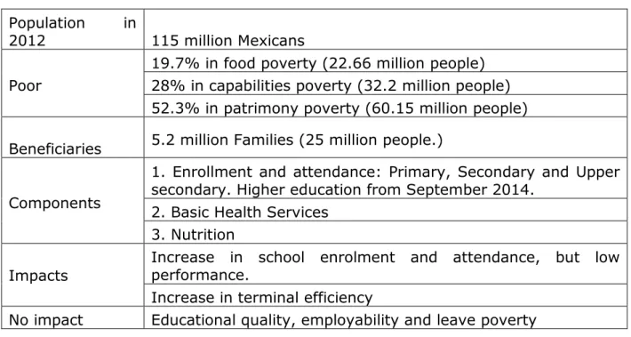
Table 1 shows a summary of the impacts; as we can observe almost 25% of Mexican population is beneficiary of Oportunidades, this is almost 50% of the poor population.

Table 1. Oportunidades Beneficiaries

Population in

2012 115 million Mexicans

Poor

19.7% in food poverty (22.66 million people) 28% in capabilities poverty (32.2 million people) 52.3% in patrimony poverty (60.15 million people)

Beneficiaries 5.2 million Families (25 million people.)

Components

1. Enrollment and attendance: Primary, Secondary and Upper secondary. Higher education from September 2014.

2. Basic Health Services 3. Nutrition

Impacts

Increase in school enrolment and attendance, but low performance.

Increase in terminal efficiency

No impact Educational quality, employability and leave poverty

The debate about conditional cash transfers impacting in labor force participation has been long, some researches argue that the behavior change because household heads are no willing to leave this benefit and inhibits mothers participation. (Freije, Bando & Arce, 2006). Therefore, the program has not been able to impact in poverty reduction even when the number of beneficiaries has increase in time (see graph 6).

10

Graph 6. Families supported by Oportunidades

Source: Author elaboration with Oportunidades data.

At the same time the Budget of the program is currently more than 63,000 million pesos (2014), and in 2013 was a 36,177 million, in 2012 34,941 million.

Graph 7. Oportunidades Budget (millions of MXP)

Source: Author elaboration with Oportunidades data.

2.5

3.2

4.2

4.2

5

5

2000

2001

2002

2003

2004

2005

11

3. A proposal of Earned Income Tax Credit (EITC)

The public policy of EITC has been implemented since 1975 in United States; it is a reimbursed fiscal credit that rewards the laborer in a household. The target population is low income families. The amount of the credit is calculated based on labor income, and conditional on workers labor participation counting the total taxable income. If the credit is higher than the tax, the family receives a cash transfer in their annual income declaration, (bibliography).

The benefit that each family receives depends on their level of income, marriage status, and number of eligible children. There are three segments to be considered to provide the benefits: the first segment. (phase in), the second segment (flat region) and the third segment (phase out) (see graph 9). In the first segment the EITC behave like a subsidy proportional to wage, and in the second segment it is a fix amount, the third segment is proportional to income and is decreasing as income increases. Married couples with a working partner have higher benefits in the second and third segments, in order not to disincentives employment.

Graph 8: Earned Income Tax Credit

12

Graph 9: Effect of EITC and CCT on budget restriction

Source: (Agostini, Selman, & Perticará, 2013)

This graph presents the Budget restriction of a single parent family (or with a single worker). “Before EITC” reflects the situation where a person is except of paying taxes. The initial situation, EITC nor the CCT program for a person that does not work is in point A, with a welfare level corresponding to curve𝑢0.

Receiving a CCT expands the non-labor income, and allow the person that do not work to reach a higher welfare level, for instance in 𝑢1. If the person works in the initial state, the CCT would have an income

effect that will be associated to an increase in leisure hours (reducing his working hours) and increasing his consumption. On the other hand, the person that does not work before and after the EITC will stay in point A after the credit is applied, but if he decides to work will have Access to a higher welfare level, for example 𝑢1. Therefore, at the end for the same level of welfare, 𝑢1, a CCT program, allow the person to

reach point B, and EITC that incentive work make it possible to reach point C. (Agostini, Selman, & Perticará, 2013). B C A Phase out w(1-t) Flat region w Phase in w(1+t)

13

4. Data and simulation methodology

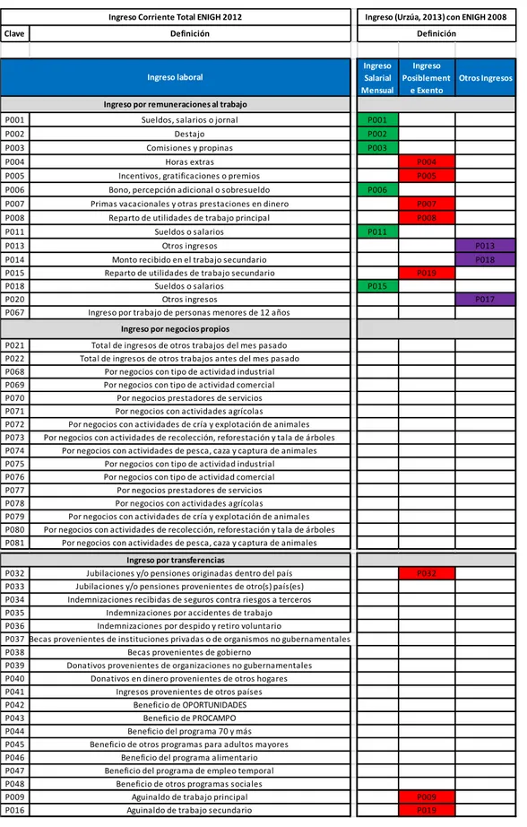
We replicate the methodology used in Selman et. al. (2013) with Mexican data, so that we can compare our results to theirs. The simulation consists in four consecutive stages: First we calculate the taxable income and the amount of tax that each person should pay because the EITC is calculated using the wage and the rest of the taxable income.6 To predict the labor income of those that do not work we estimate a wage equation in logs using Heckman (1979) selection equation.7 Estimating this equation corrects the bias caused by the decision of participating in the labor force. Figure 2 shows the two official definitions of taxable income used by two Mexican government institutions. We will use the one that CONEVAL used to calculate net income to define poverty measures, and we consider the tax rates of the treasury SHCP.

Figure 2. Taxable Income according to several definitions

Source: Ortega & Castellanos (2014)

6

We can see the codes for each income that is taxable in the appendix.

7

The first stage consists in estimating a Probit model of labor participation: 𝑃𝑟𝑜𝑏(𝑆𝑖= 1| 𝑍𝑖) = Φ(𝑍𝑖𝛾)

S equals one for those who work, and Z is a vector of socioeconomic variables that determine whether the person would work or not. In the second stage consist in estimating the amount of wage and the Mills ratio is introduced as regressor:

𝐸(𝑌𝑖| 𝑋𝑖, 𝑍𝑖, 𝑆𝑖= 1) = 𝑋𝑖𝛽 + 𝜌𝜆(𝑍𝑖𝛾), con 𝜆(𝑍𝑖𝛾) = ϕ(𝑍_Φ(𝑍𝑖𝛾)

𝑖𝛾)

For those who do not work we assume a distribution of the error with zero mean and variance equal to the variance of the error of people that work.

Investments

Income

Gross Income

Net Income

Interest on fixed

maturities, from

savings accounts and

loans, (pp.97)

Labor income, income from professional activities and

rentals, income from corporate activities, interests and contributions

to social security, (pp. 95)

SHCP

Labor income income from professional activities and rentals, income from corporate activities and interests,

(pp. 96)

Interests from fixed terms investments, interests from loans, interests from saving accounts and yields from

bonds and warrants.

Monetary income

plus the non

monetary income.

CONEVAL

Monetary income

plus the non

monetary income,

minus the gifts given

14

The second step consists in calculating the annual amount of credit to be reimbursed to those female workers that accomplish the EITC requirements based on age, number of children and income. This amount depends on the hours worked for those who participate in the labor market. For those who do not work, the wage prediction is used and we assume they work between 20 and 45 hours weekly.

In the third stage, once we have the amount of tax credit, the income tax to be paid and the net income, together with the percentage variation with respect to the initial income of all eligible people, we identified the beneficiaries of the program. For this paper we concentrate in women that work and are eligible so that they will be beneficiaries. In the case of eligible women that do not work, we use the labor participation elasticity and the percentage variation of income, and calculate the probability of participation after applying EITC. If the new probability is higher than 0.5 we assumed that the person will enter the labor force, and receive EITC. One strong assumption is that, as in Selman et.al (2013), there is labor demand for women who want to work. This may affect women´s wage due to competing in the market for a job. Notwithstanding a minimum wage should be set as a floor, in the case of Mexico this is relevant as the labor reform and the initiatives are voting in favor of raising minimum wage.

In their review, Selman et.al (2013), identify two effects of implementing EICT. The first effect in the hour labor supply (intensive margin), the second in labor participation. In a first implementation of EICT, the in the number of working hours is relevant for those who are already working, and not for those who insert into the labor marked as consequence of EITC program. If hour’s elasticity is ℇ𝑘, the number of working hours supplied by each worker after implementing EITC is defined as:

𝐻𝑜𝑢𝑟𝑠𝐸𝐼𝑇𝐶 = 𝐻𝑜𝑢𝑟𝑠0(1 + ℇ𝑘∙ 𝑐ℎ𝑎𝑛𝑔𝑒 𝑖𝑛 𝑙𝑎𝑏𝑜𝑟 𝑖𝑛𝑐𝑜𝑚𝑒).

Notwithstanding, the elasticity of participation with respect to wage net of taxes is higher than the elasticity of hours supplied, and considering alone ℇ𝑘 can bias the effects of the program in a simulation as it is difficult for an average worker to modify its labor hours.

Selman et.al (2013), uses the Meyer (2007) assumptions about the EICT increasing labor supply and not decreasing the intensity of labor, therefore we assume in the beginning a non-compensated elasticity of labor supply equal to zero (ℇ𝑘 = 0), and for sensibility analysis this will be changed to 0.1, and describe the change in results.

To estimate the labor participation we use the results of the Heckman probability equation and then calculate the marginal effect of each variable on the labor participation 𝜕𝑃𝑟𝑜𝑏(𝑆_{𝜕 log(𝑧}𝑖=1)

𝑗) = 𝜙(𝑍𝑖𝛾) ∙ 𝛾𝑗.

This change in an independent variable, that was initially zero modifies the probability of participate in the labor market. Therefore, if 𝛾𝑘 is the elasticity of participation, the change in the probability of participation due to EITC for those who do not work initially will be calculated using the following definition.

𝑃𝑟𝑜𝑏(𝑆_{𝐸𝐼𝑇𝐶}= 1) = Φ(𝑍_𝑖𝛾) + 𝜙(𝑍_𝑖𝛾) ∙ 𝛾_𝑘∙ log (𝑐ℎ𝑎𝑛𝑔𝑒 𝑖𝑛 𝑙𝑎𝑏𝑜𝑟 𝑖𝑛𝑐𝑜𝑚𝑒),

Where the change in labor income is the sum of the monthly wage and the EITC received, discounting the unemployment benefits forgone in case of joining the labor force. Afterwards, as we aid before, we assume than if the probability is higher than 0.5, 𝑃𝑟𝑜𝑏(𝑆𝐸𝐼𝑇𝐶 = 1) ≥ 0.5, people will join the labor force.

15

Labor income (𝑧𝑘) is initially zero for those women who do not work and it becomes positive when the person works after the EITC program is implemented. If they work, the labor income is the sum of workers wage and the amount of EITC received.

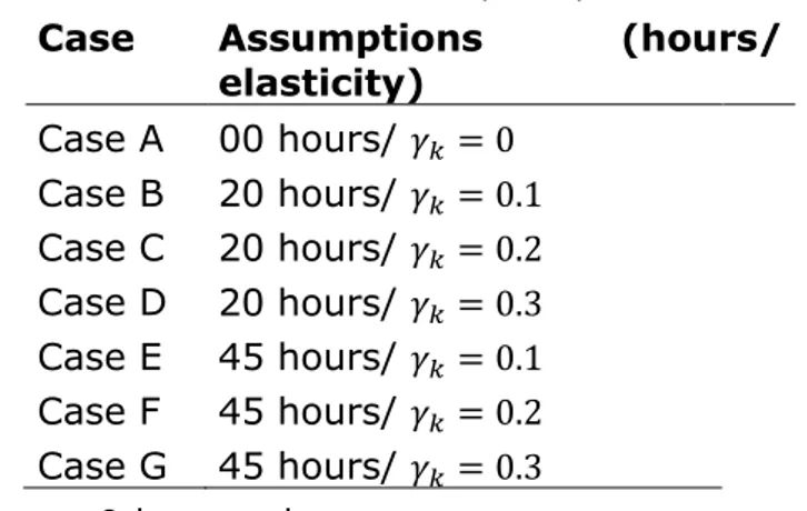
The simulations will be performed using the values 0, 0.1, 0.2, 0.3 for women elasticity participation.8

We use seven different simulations for the number of working hours that new incomers in the labor market supply (20 to 45 hours), combined with the four different values of the elasticity of labor participation. In all the cases it is assumed an initial elasticity of hours equal to zero (ℇ𝑘 = 0).

In table 2 we describe the cases to be simulated. The first one, in which there is a zero elasticity (ℇ𝑘 = 0), assumes people do not modify their behavior towards labor income changes, and only those initially working continue to work. The rest of the cases consider labor insertion after implementing EITC.

Table 2: Hours of work and labor participation elasticities Case Assumptions (hours/

elasticity) Case A 00 hours/ 𝛾𝑘 = 0 Case B 20 hours/ 𝛾_𝑘 = 0.1 Case C 20 hours/ 𝛾𝑘 = 0.2 Case D 20 hours/ 𝛾_𝑘 = 0.3 Case E 45 hours/ 𝛾_𝑘 = 0.1 Case F 45 hours/ 𝛾_𝑘 = 0.2 Case G 45 hours/ 𝛾_𝑘 = 0.3 Source: Selman et. al.

The fourth and last stage of the simulations consists in analysis the income distribution after each case. With this data is possible to identify the effect of implementing EITC in labor participation, and in different indicators of poverty and inequality.

Data

First we calculate the taxable income using table A1 of the appendix and estimate the different type of household in each bracket. Their socioeconomics characteristics and make the essential corrections to control for the outliers with respect to wage and hours worked.

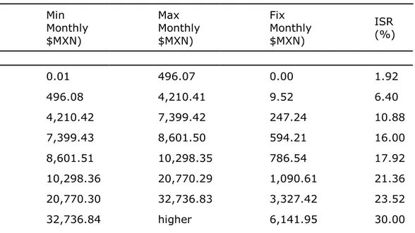
In the second stage we calculate the income tax limits using the Income Tax Law published in the Official Journal of the Mexican Federation on May 25th 2012, which establishes that the tax amount to be paid should abide to the limits in Table 3. Where TA is the Tax Amount to be paid, FA is a Fixed Amount, ISR is the Income Tax Rate, I is the earned income and BL is the Lower Bound. Earned Income (I) determines the FA and the ISR according the bracket.

*(

)

i i i i i

TA



FA



ISR

I



BL

8 _{The selection of these values is based in Eissa and Hoynes (2006). These values are moderate so that the results}

16 Table 3 Limits of the income tax (ISR)

Min Monthly $MXN) Max Monthly $MXN) Fix Monthly $MXN) ISR (%) 0.01 496.07 0.00 1.92 496.08 4,210.41 9.52 6.40 4,210.42 7,399.42 247.24 10.88 7,399.43 8,601.50 594.21 16.00 8,601.51 10,298.35 786.54 17.92 10,298.36 20,770.29 1,090.61 21.36 20,770.30 32,736.83 3,327.42 23.52 32,736.84 higher 6,141.95 30.00

Source: Tax Law of Mexico, 2012

Table 4 Limits for tax subsidies Min Monthly $MXN Max Monthly $MXN Fix Employment Subsidy, Monthly $MXN 0.01 1,768.96 407.02 1,768.97 2,653.38 406.83 2,653.39 3,472.84 406.62 3,472.85 3,537.87 392.77 3,537.88 4,446.15 382.46 4,446.16 4,717.18 354.23 4,717.19 5,335.42 324.87 5,335.43 6,224.67 294.63 6,224.68 7,113.90 253.54 7,113.91 7,382.33 217.61 7,382.34 And higher 0.00

17

In order for this research to be comparable in the future with the Chilean case of earned income tax credit done in Selman et. al. (2013) we define the parameters based in EITC scheme of US in 19969 _and we adjust by the rate between GDP-1996 and the GDP-2012 (year of the simulation for Mexico). In the tables 3 to 5 we present the parameters used. In the appendix is table A2 for the case of Chile.

2012 2012

*

_

MXN USD MXN USD

EITC



EITC

Exchange rate

2009 1996

*

_

CLP USD CLP USD

EITC



EITC

Exchange rate

2012 1996 2012/ 2012 2012 1996/

*

_

EITC

Exchange rate

EITC

GDP



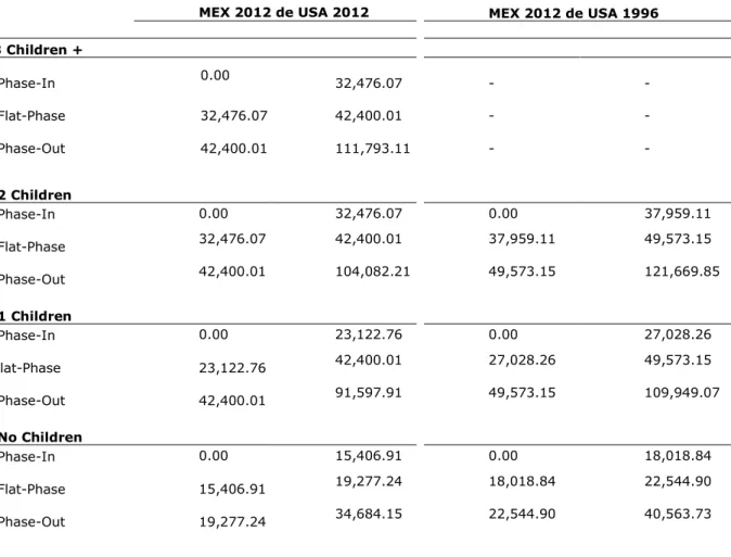
Table 5 Limits for Annual EITC that households should receive by income level

MEX 2012 de USA 2012 MEX 2012 de USA 1996

3 Children + Phase-In 0.00 32,476.07 - - Flat-Phase 32,476.07 42,400.01 - - Phase-Out 42,400.01 111,793.11 - - 2 Children Phase-In 0.00 32,476.07 _0.00 37,959.11 Flat-Phase 32,476.07 42,400.01 37,959.11 49,573.15 Phase-Out 42,400.01 104,082.21 49,573.15 121,669.85 1 Children Phase-In 0.00 23,122.76 0.00 27,028.26 Flat-Phase 23,122.76 42,400.01 27,028.26 49,573.15 Phase-Out 42,400.01 91,597.91 49,573.15 109,949.07 No Children Phase-In 0.00 15,406.91 0.00 18,018.84 Flat-Phase 15,406.91 19,277.24 18,018.84 22,544.90 Phase-Out 19,277.24 34,684.15 22,544.90 40,563.73

9 _{The scheme is the first after the expansion in 1993. From 1996 the rates have been kept relatively constant and}

the amounts of transfers have increased slowly. We do not use the amounts of 2009 because their increased is not comparable with Chilean economy. The table A2 in the appendix shows the parameters of EITC in 1996.

18 Exchange rate $13.17 $13.17 GDPpcUSA2012 /GDPpcMEX2012 5.308 3.084

Source: Ortega, Castellanos & Islas (2014)

Therefore the EITC will be the following considering a 2012 exchange rate.

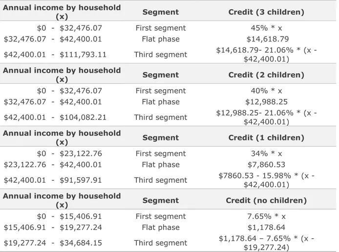
Table 6: Income schedule, Rates and Credit amount proposed for Mexico

Annual income by household

(x) Segment Credit (3 children)

$0 - $32,476.07 First segment 45% * x $32,476.07 - $42,400.01 Flat phase $14,618.79

$42,400.01 - $111,793.11 Third segment $14,618.79- 21.06% * (x - _$42,400.01)

Annual income by household

(x) Segment Credit (2 children)

$0 - $32,476.07 First segment 40% * x $32,476.07 - $42,400.01 Flat phase $12,988.25

$42,400.01 - $104,082.21 Third segment $12,988.25- 21.06% * (x - _$42,400.01)

Annual income by household

(x) Segment Credit (1 children)

$0 - $23,122.76 First segment 34% * x $23,122.76 - $42,400.01 Flat phase $7,860.53

$42,400.01 - $91,597.91 Third segment $7860.53 - 15.98% * (x - _$42,400.01)

Annual income by household

(x) Segment Credit (no children)

$0 - $15,406.91 First segment 7.65% * x $15,406.91 - $19,277.24 Flat phase $1,178.64

$19,277.24 - $34,684.15 Third segment $1,178.64 – 7.65% * (x - _$19,277.24)

19

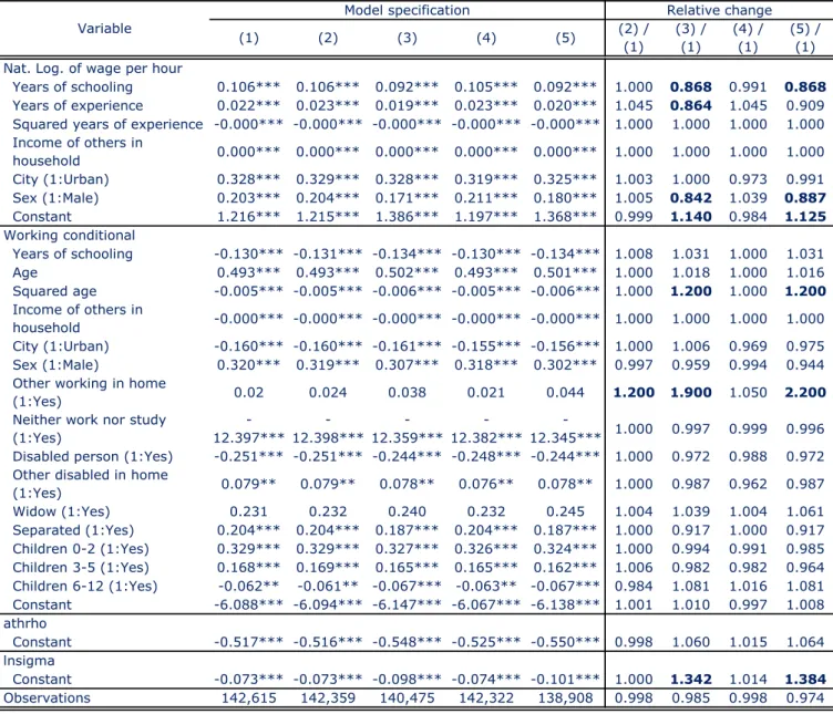
Table Heckman equation estimation and analysis of relative change

Variable

Model specification Relative change

(1) (2) (3) (4) (5) (2) / (1) (3) / (1) (4) / (1) (5) / (1) Nat. Log. of wage per hour

Years of schooling 0.106*** 0.106*** 0.092*** 0.105*** 0.092*** 1.000 0.868 0.991 0.868

Years of experience 0.022*** 0.023*** 0.019*** 0.023*** 0.020*** 1.045 0.864 1.045 0.909 Squared years of experience -0.000*** -0.000*** -0.000*** -0.000*** -0.000*** 1.000 1.000 1.000 1.000 Income of others in household 0.000*** 0.000*** 0.000*** 0.000*** 0.000*** 1.000 1.000 1.000 1.000 City (1:Urban) 0.328*** 0.329*** 0.328*** 0.319*** 0.325*** 1.003 1.000 0.973 0.991 Sex (1:Male) 0.203*** 0.204*** 0.171*** 0.211*** 0.180*** 1.005 0.842 1.039 0.887 Constant 1.216*** 1.215*** 1.386*** 1.197*** 1.368*** 0.999 1.140 0.984 1.125 Working conditional Years of schooling -0.130*** -0.131*** -0.134*** -0.130*** -0.134*** 1.008 1.031 1.000 1.031 Age 0.493*** 0.493*** 0.502*** 0.493*** 0.501*** 1.000 1.018 1.000 1.016 Squared age -0.005*** -0.005*** -0.006*** -0.005*** -0.006*** 1.000 1.200 1.000 1.200 Income of others in household -0.000*** -0.000*** -0.000*** -0.000*** -0.000*** 1.000 1.000 1.000 1.000 City (1:Urban) -0.160*** -0.160*** -0.161*** -0.155*** -0.156*** 1.000 1.006 0.969 0.975 Sex (1:Male) 0.320*** 0.319*** 0.307*** 0.318*** 0.302*** 0.997 0.959 0.994 0.944 Other working in home

(1:Yes) 0.02 0.024 0.038 0.021 0.044 1.200 1.900 1.050 2.200

Neither work nor study (1:Yes) -12.397*** -12.398*** -12.359*** -12.382*** -12.345*** 1.000 0.997 0.999 0.996 Disabled person (1:Yes) -0.251*** -0.251*** -0.244*** -0.248*** -0.244*** 1.000 0.972 0.988 0.972 Other disabled in home

(1:Yes) 0.079** 0.079** 0.078** 0.076** 0.078** 1.000 0.987 0.962 0.987 Widow (1:Yes) 0.231 0.232 0.240 0.232 0.245 1.004 1.039 1.004 1.061 Separated (1:Yes) 0.204*** 0.204*** 0.187*** 0.204*** 0.187*** 1.000 0.917 1.000 0.917 Children 0-2 (1:Yes) 0.329*** 0.329*** 0.327*** 0.326*** 0.324*** 1.000 0.994 0.991 0.985 Children 3-5 (1:Yes) 0.168*** 0.169*** 0.165*** 0.165*** 0.162*** 1.006 0.982 0.982 0.964 Children 6-12 (1:Yes) -0.062** -0.061** -0.067*** -0.063** -0.067*** 0.984 1.081 1.016 1.081 Constant -6.088*** -6.094*** -6.147*** -6.067*** -6.138*** 1.001 1.010 0.997 1.008 athrho Constant -0.517*** -0.516*** -0.548*** -0.525*** -0.550*** 0.998 1.060 1.015 1.064 lnsigma Constant -0.073*** -0.073*** -0.098*** -0.074*** -0.101*** 1.000 1.342 1.014 1.384 Observations 142,615 142,359 140,475 142,322 138,908 0.998 0.985 0.998 0.974

Source: Ortega, Castellanos & Islas (2014)

Note: Bold values indicate a relative change higher than 10% (Black for positive and red for negative)

* p<0.05, ** p<0.01, *** p<0.001

(1) Whole sample

(2) Excluding outliers in working hours

(3) Excluding outliers in individual annually labor income (4) Excluding outliers in income of other household members (5) Excluding outlier of (2), (3) and (4)

5. Estimation Results

We specify five different models

Table 7

Simulation 1: Whole sample

Using the whole sample of women between 16 and 65 years old we predict the wage that the worker will have in case she inserted to the labor force. The probability of working should be higher than 50%.

20

We have that from 18,417,683 women working, with the selection equation 19,108,147 would work, this means that 690,464 female workers would be inserted into the labor force. Let’s see what happen if EITC were implemented to all workers.

Table 8

Variable Obs Mean Std. Dev. Min Max

Taxable Income 39432 4088.695 7159.789 0 670134.4 Sim Tax Income 68437 2940.845 6062.019 0 670134.4

Tax 39431 419.1763 1693.384 .1369509 197361.2 Annual tax 39431 5030.115 20320.61 1.64341 2368335 Tax sim 1 67510 2879.54 3214.976 .1369509 197361.2 Annual tax sim1 67510 34554.48 38579.71 1.64341 2368335

6. Conclusions

Without EITC the poverty of women (16-65 year old) was higher:

Without EITC With EITC Difference

Women Poor % Women Poor % Women Poor %

Food poverty 6,627,883 17.27 2,499,491 8.21 -4,128,392 -9.06 Capabilities poverty 9,338,758 24.33 9,338,758 24.33 0 0 Patrimony poverty 18,262,106 47.57 18,262,106 47.57 0 0

EITC is a better option to tackle poverty. Mainly for the following reasons:

 Cost less than Oportunidades (95,173,665 MXP a year)

 Is quicker.

 Is sustainable as is a formal work.

 Reduces more poverty rates.

 Have worker that make pension system more suitable.

21

7. Appendix

Table A1. Taxable Income Codes for Mexico that are comparable with Chile

Source: Ortega & Castellanos (2014)

Clave Definición Ingreso Salarial Mensual Ingreso Posiblement e Exento Otros Ingresos

P001 Sueldos, salarios o jornal P001

P002 Destajo P002

P003 Comisiones y propinas P003

P004 Horas extras P004

P005 Incentivos, gratificaciones o premios P005

P006 Bono, percepción adicional o sobresueldo P006

P007 Primas vacacionales y otras prestaciones en dinero P007 P008 Reparto de utilidades de trabajo principal P008

P011 Sueldos o salarios P011

P013 Otros ingresos P013

P014 Monto recibido en el trabajo secundario P018

P015 Reparto de utilidades de trabajo secundario P019

P018 Sueldos o salarios P015

P020 Otros ingresos P017

P067 Ingreso por trabajo de personas menores de 12 años

P021 Total de ingresos de otros trabajos del mes pasado P022 Total de ingresos de otros trabajos antes del mes pasado P068 Por negocios con tipo de actividad industrial P069 Por negocios con tipo de actividad comercial P070 Por negocios prestadores de servicios P071 Por negocios con actividades agrícolas

P072 Por negocios con actividades de cría y explotación de animales P073 Por negocios con actividades de recolección, reforestación y tala de árboles P074 Por negocios con actividades de pesca, caza y captura de animales P075 Por negocios con tipo de actividad industrial P076 Por negocios con tipo de actividad comercial P077 Por negocios prestadores de servicios P078 Por negocios con actividades agrícolas

P079 Por negocios con actividades de cría y explotación de animales P080 Por negocios con actividades de recolección, reforestación y tala de árboles P081 Por negocios con actividades de pesca, caza y captura de animales

P032 Jubilaciones y/o pensiones originadas dentro del país P032 P033 Jubilaciones y/o pensiones provenientes de otro(s) país(es)

P034 Indemnizaciones recibidas de seguros contra riesgos a terceros P035 Indemnizaciones por accidentes de trabajo P036 Indemnizaciones por despido y retiro voluntario

P037 Becas provenientes de instituciones privadas o de organismos no gubernamentales P038 Becas provenientes de gobierno

P039 Donativos provenientes de organizaciones no gubernamentales P040 Donativos en dinero provenientes de otros hogares P041 Ingresos provenientes de otros países P042 Beneficio de OPORTUNIDADES

P043 Beneficio de PROCAMPO

P044 Beneficio del programa 70 y más P045 Beneficio de otros programas para adultos mayores P046 Beneficio del programa alimentario P047 Beneficio del programa de empleo temporal P048 Beneficio de otros programas sociales

P009 Aguinaldo de trabajo principal P009

P016 Aguinaldo de trabajo secundario P019

Ingreso por negocios propios

Ingreso por transferencias

Ingreso Corriente Total ENIGH 2012 Ingreso (Urzúa, 2013) con ENIGH 2008 Definición

Ingreso laboral Ingreso por remuneraciones al trabajo

22

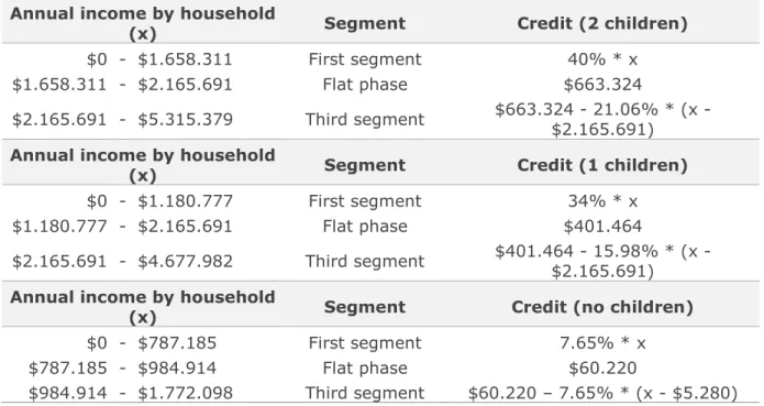
Table A2: Income schedule, Rates and Credit amount proposed for Chile

Annual income by household

(x) Segment Credit (2 children)

$0 - $1.658.311 First segment 40% * x $1.658.311 - $2.165.691 Flat phase $663.324

$2.165.691 - $5.315.379 Third segment $663.324 - 21.06% * (x - _$2.165.691)

Annual income by household

(x) Segment Credit (1 children)

$0 - $1.180.777 First segment 34% * x $1.180.777 - $2.165.691 Flat phase $401.464

$2.165.691 - $4.677.982 Third segment $401.464 - 15.98% * (x - _$2.165.691)

Annual income by household

(x) Segment Credit (no children)

$0 - $787.185 First segment 7.65% * x

$787.185 - $984.914 Flat phase $60.220

$984.914 - $1.772.098 Third segment $60.220 – 7.65% * (x - $5.280) Source: Selman et. al.

Tabla A3: Tamaño del crédito por nivel de ingresos (US$) y nº de hijos (1996)

Ingreso del Hogar (x)

Segmento

Credit (2 children)

$0 – $8.890

Primer segment

40% * x

$8.890 – $11.610

Phase flat

$3.556

$11.610 – $28.495

Third segment

$3.556 - 21.06% * (x - $11.610)

Household Income (x)

Segment

Credit (1 child)

$0 – $6.330

Primer segment

34% * x

$6.330 – $11.610

Phase flat

$2.152

$11.930 – $25.750

Third segment

$2.152 - 15.98% * (x - $11.610)

Income of the

Household (x)

Segment

Credit (sin children)

$0 – $4.220

Primer segment

7.65% * x

$4.220 – $5.280

Phase flat

$323

$5.280 – $9.500

Third segment

$323 – 7.65% * (x - $5.280)

23

Table A4: Tamaño del crédito por nivel de ingresos (US$) y nº de hijos (2009)

Income of the Household

(x)

Segment

Credit (3 ó + children)

$0 – $12.570

Primer segment

45% * x

$12.570 – $16.420

Phase flat

$ 5.657

$16.420 – $43.279

Third segment

$5.657 - 21.06% * (x - $16.420)

Income of the Household

(x)

Segment

Credit (2 children)

$0 – $12.570

Primer segment

40% * x

$12.570 – $16.420

Phase flat

$ 5.028

$16.420 – $40.295

Third segment

$5.028 - 21.06% * (x - $16.420)

Income of the Household

(x)

Segment

Credit (1 child)

$0 – $8.950

Primer segment

34% * x

$8.950 – $16.420

Phase flat

$ 3.043

$16.420 – $35.463

Third segment

$3.043 - 15.98% * (x - $16.420)

Income of the Household

(x)

Segment

Credit (sin children)

$0 – $5.970

Primer segment

7.65% * x

$5.970 – $7.470

Phase flat

$ 457

$7.470 – $13.440

Third segment

$457 – 7.65% * (x - $7.470)

Note: From 2009, there is a difference in EITC from 2 to 3 children or more. Source: Selman et. al.http://www.irs.gov

24

8. Bibliography

Agostini, C., Selman, J., & Perticará, M. (2013). Una Propuesta de Crédito Tributario al Ingreso Para Chile.

Estudios Públicos, 129, 49-104.

Campos B., P. (2012). Documento Compilatorio de la Evaluación Externa 2007-2008 del Programa

Oportunidades Mexico: Sedesol Retrieved from

https://www.prospera.gob.mx/EVALUACION/es/wersd53465sdg1/docs/2010/2010_doc_compil atorio2008.pdf.

Freije, Bando & Arce (2006) Conditional Transfers,Labor Supply, and Poverty:Microsimulating Oportunidades. E C O N O M I A.

INSP. (2014). NOTA EXPLICATIVA SOBRE LA INTERPRETACIÓN DE LA COMPARACIÓN DE RESULTADOS EN

INDICADORES DE SALUD Y/O NUTRICIÓN ENTRE LA POBLACIÓN BENEFICIARIA Y LA NO BENEFICIARIA DE OPORTUNIDADES EN LA ENCUESTA NACIONAL DE SALUD Y NUTRICIÓN

(ENSANUT) 2011 - 2012. Sedesol Retrieved from

https://www.prospera.gob.mx/EVALUACION/es/wersd53465sdg1/docs/2012/nota_ensanut_201 1_2012.pdf.

Jere R. Behrman, Piyali Sengupta, & Petra Todd. (2005). Progressing through PROGRESA: An Impact Assessment of a School Subsidy Experiment in Rural Mexico. Economic Development and Cultural

Change, 54(1), 237-275.

López P., O. (2012). Evaluación del Proyecto Estímulos para el Desarrollo Humano y las Capacidades de

los Adultos (EDHUCA) 2012. Mexico: El Colegio de San Luis Ac.

Ortega D., A. (2014). Describiendo el Mercado Laboral Mexicano utilizando un Índice Multidimensional de

Trabajo Decente para México (L. Treviño Ed.): Universidad Autónoma de Nuevo León.

Ortega Díaz, A. (2013). Defining a Multidimensional Index of Decent Work for México. The Mexican Journal of Economics and Finance, 8(1).

Ortega-Díaz, A., & Vilalta, C. (2012). The Challenge of Inequality and Poverty. In T. d. Monterrey (Ed.),

Building a Future for Mexico (Vol. 1). Mexico: Tecnológico de Monterrey.

Valora. (2012). El desempeño de los becarios del Programa Oportunidades en la prueba ENLACE: cambios

entre 2008 y 2011 en educación básica y media superior. . Mexico: Retrieved from

https://www.prospera.gob.mx/EVALUACION/es/wersd53465sdg1/docs/2012/valora_desemp_b ecarios_prueba_enlace_vf.pdf.

21

NOPOOR

®

NOPOOR Project

Research for change : More than 100 researchers from all over the world explore innovative methods to

fight for better living conditions in Africa, Asia and Latin America.

Evidence-based Advise : The project brings new knowledge to policy makers and other stakeholders in the

field of poverty alleviation – donors and beneficiaries, civil society and researchers, development

practitioners and media.

More than 100 researchers from 20 institutions worldwide.

www.nopoor.eu

© NOPOOR, 2014